UCLA
UCLA Electronic Theses and Dissertations
TitleTask-oriented Visual Understanding for Scenes and Events Permalink https://escholarship.org/uc/item/0qb0005c Author Qi, Siyuan Publication Date 2019 Peer reviewed|Thesis/dissertation
UNIVERSITY OF CALIFORNIA Los Angeles
Task-oriented Visual Understanding for Scenes and Events
A dissertation submitted in partial satisfaction of the requirements for the degree Doctor of Philosophy in Computer Science
by Siyuan Qi
c
Copyright by Siyuan Qi
ABSTRACT OF THE DISSERTATION
Task-oriented Visual Understanding for Scenes and Events by
Siyuan Qi
Doctor of Philosophy in Computer Science University of California, Los Angeles, 2019
Professor Song-Chun Zhu, Chair
Scene understanding and event understanding of humans correspond to the spatial and temporal aspects of computer vision. Such abilities serve as a foundation for humans to learn and perform tasks in the world we live in, thus motivating a task-oriented represen-tation for machines to interpret observations of this world.
Toward the goal oftask-oriented scene understanding, I begin this thesis by presenting
a human-centric scene synthesis algorithm. Realistic synthesis of indoor scenes is more complicated than neatly aligning objects; the scene needs to be functionally plausible, which requires the machine to understand the tasks that could be performed in the scene.
Instead of directly modeling the object-object relationships, the algorithm learns the human-object relations and generate scene configurations by imagining the hidden human factors in the scene. I analyze the realisticity of the synthesized scenes, as well as its usefulness for various computer vision tasks. This framework is useful for backward in-ference of 3D scenes structures from images in an analysis-by-synthesis fashion; it is also useful for generating data to train various algorithms.
parsing, event prediction, and task planning. In the computer vision literature, event un-derstanding usually refers to action recognition from videos, i.e., “what is the action of
the person”. Task-oriented event understanding goes beyond this definition to find out the underlying driving forces of other agents. It answers questions such as intention recogni-tion (“what is the person trying to achieve”), and intenrecogni-tion predicrecogni-tion (“how the person is going to achieve the goal”), from a planning perspective.
The core of this framework lies in the temporal representation for tasks that is ap-propriate for humans, robots, and the transfer between these two. In particular, inspired by natural language modeling, I represent the tasks by stochastic context-free grammars, which are natural choices to capture the semantics of tasks, but traditional grammar parsers (e.g., Earley parser) only take symbolic sentences as inputs. To overcome this drawback,
I generalize the Earley parser to parse sequence data which is neither segmented nor la-beled. This generalized Earley parser integrates a grammar parser with a classifier to find the optimal segmentation and labels. It can be used for event parsing, future predictions, as well as incorporating top-down task planning with bottom-up sensor inputs.
The dissertation of Siyuan Qi is approved.
Ying Nian Wu Demetri Terzopoulos
Kai-Wei Chang
Song-Chun Zhu, Committee Chair
University of California, Los Angeles 2019
TABLE OF CONTENTS
1 Introduction. . . 1
2 Human-centric Indoor Scene Synthesis Using Stochastic Grammar . . . 4
2.1 Introduction . . . 6
2.2 Related Work . . . 11
2.3 Representation and Formulation . . . 15
2.3.1 Representation: Attributed Spatial And-Or Graph . . . 15
2.4 Probabilistic Formulation of S-AOG . . . 19
2.5 Learning, Sampling and Synthesis . . . 24
2.5.1 Learning the S-AOG . . . 25
2.5.2 Sampling Scene Geometry Configurations . . . 28
2.5.3 Scene Instantiation using 3D Object Datasets . . . 33
2.5.4 Scene Attribute Configurations . . . 34
2.6 Photorealistic Scene Rendering . . . 35
2.7 Experiments . . . 40
2.7.1 Realisticity of Sampled Scene Configurations . . . 40
2.7.2 Synthesized Indoor Scene Data for Scene Understanding . . . 47
2.8 Discussion . . . 56
2.9 Conclusion and Future Work . . . 60
3 Human Activity Prediction Using Stochastic Grammar . . . 71
3.1 Related Work . . . 76
3.2 Representation: Probabilistic Context-Free Grammars . . . 79
3.3 Earley Parser . . . 80
3.4 Generalized Earley Parser . . . 85
3.4.1 Parsing Operations . . . 88
3.4.2 Parsing & Prefix Probability Formulation . . . 90
3.4.3 Incorporating Grammar Prior . . . 91
3.4.4 Segmentation and Labeling . . . 96
3.4.5 Future Label Prediction . . . 96
3.5 Human Activity Parsing and Prediction . . . 99
3.5.1 Grammar Induction . . . 100
3.5.2 Experiment on CAD-120 Dataset . . . 101
3.5.3 Experiment on Watch-n-Patch Dataset . . . 103
3.5.4 Experiment on Breakfast Dataset . . . 106
3.5.5 Discussion . . . 108
3.6 Conclusion . . . 111
4 Conclusion . . . 112
LIST OF FIGURES
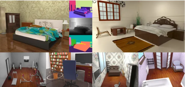
2.1 An example of synthesized indoor scene (bedroom) with affordance heatmap. The joint sampling of a scene is achieved by alternative sampling of humans and objects according to the joint probability distribution. . . 5 2.2 (Top Left) An example automatically-generated 3D bedroom scene, rendered
as a photorealistic RGB image, along with per-pixel ground truth of surface normal, depth, and object identity. (Top Right) Another synthesized bedroom scene. Synthesized scenes include fine details—objects (e.g., the duvet and
pillows on beds) and their textures are changeable, by sampling physical pa-rameters of materials (reflectance, roughness, glossiness, etc..), and
illumi-nation parameters are sampled from continuous spaces of possible positions, intensities, and colors. (Bottom) Rendered images of 4 example synthetic in-door scenes. . . 9
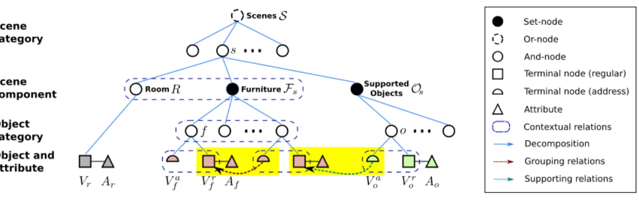
2.3 Scene grammar as an attributed S-AOG. A scene of different types is decom-posed into a room, furniture, and supported objects. Attributes of terminal nodes are internal attributes (sizes), external attributes (positions and orien-tations), and a human position that interacts with this entity. Furniture and object nodes are combined by an address terminal node and a regular terminal node. A furniture node (e.g., a chair) is grouped with another furniture node
(e.g., a desk) pointed by its address terminal node. An object (e.g., a monitor)
is supported by the furniture (e.g., a desk) it is pointing to. If the value of
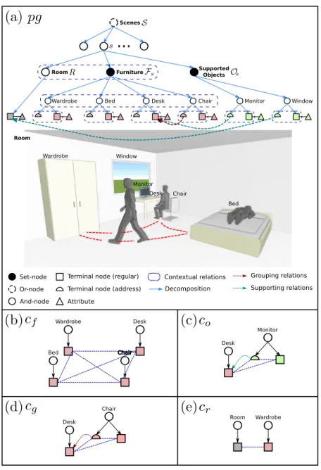
the address node is null, the furniture is not grouped with any furniture, or the object is put on the floor. Contextual relations are defined between the room and furniture, between a supported object and supporting furniture, among different pieces of furniture, and among functional groups. . . 14 2.4 (a) A simplified example of a parse graph of a bedroom. The terminal nodes
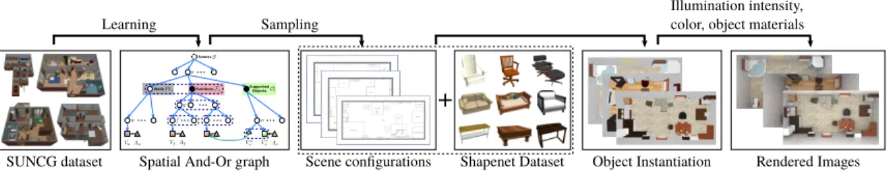
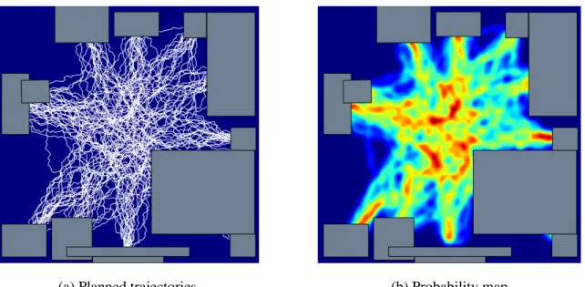
of the parse graph form an MRF in the terminal layer. Cliques are formed by the contextual relations projected to the terminal layer. Examples of the four types of cliques are shown in (b)-(e), representing four different types of contextual relations. . . 20 2.5 The learning-based pipeline for synthesizing images of indoor scenes. . . 21 2.6 Given a scene configuration, we use bi-directional RRT to plan from every
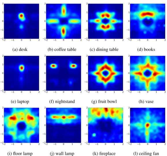
2.7 Examples of the learned affordance maps. Given the object positioned in the center facing upwards, i.e., coordinate of (0,0) facing direction (0,1), the maps show the distributions of human positions. The affordance maps accu-rately capture the subtle differences among desks, coffee tables, and dining tables. Some objects are orientation sensitive, e.g., books, laptops, and night
stands, while some are orientation invariant,e.g., fruit bowls and vases. . . . 29
2.8 MCMC sampling process (from left to right) of scene configurations with sim-ulated annealing. . . 31 2.9 Synthesis for different values ofβ. Each image shows a typical configuration
sampled from a Markov chain. . . 31 2.10 Qualitative results in different types of scenes. . . 35 2.11 We can configure the scene with different (a) illumination intensities, (b)
illu-mination colors, (c) materials, and (d) even on each object part. We can also control (e) the number of light source and their positions, (f) camera lenses (e.g., fish eye), (g) depths of field, or (h) render the scene as a panorama for
virtual reality and other virtual environments. (i) 7 different background wall textures. Note how the background affects the overall illumination. . . 36 2.12 (Continue:) we can configure the scene with different (a) illumination
intensi-ties, (b) illumination colors, (c) materials, and (d) even on each object part. We can also control (e) the number of light source and their positions, (f) camera lenses (e.g., fish eye), (g) depths of field, or (h) render the scene as a panorama
for virtual reality and other virtual environments. (i) 7 different background wall textures. Note how the background affects the overall illumination. . . . 37
2.13 Examples of scenes in ten different categories. Top: top-view. Middle: a side-view. Bottom: affordance heatmap. . . 42 2.14 (Continue:) examples of scenes in ten different categories. Top: top-view.
Middle: a side-view. Bottom: affordance heatmap. . . 43 2.15 Top-view segmentation maps for classification. . . 44 2.16 Top: previous methods [YYT11] only re-arranges a given input scene with a
fixed room size and a predefined set of objects.Bottom: our method samples a large variety of scenes. . . 45 2.17 Examples of normal estimation results predicted by the model trained with
our synthetic data. . . 48 2.18 Examples of depth estimation results predicted by the model trained with our
synthetic data. . . 51 2.19 We can render the scenes as (a) a sequence of video frames after setting
a camera trajectory, (b) which can be used to evaluate SLAM reconstruc-tion [WLS15] results. The top row shows a successful reconstrucreconstruc-tion case, while the middle and bottom rows show two failure cases due to a fast moving camera and a plain, untextured surface, respectively. . . 55 2.20 Benchmark results. (a) Given a set of generated RGB images rendered with
different illuminations and object material properties (top to bottom: origi-nal settings, with high illumination, with blue illumination, and with metallic material properties), we evaluate (b)–(d) three depth prediction algorithms, (e)–(f) two surface normal estimation algorithms, (g) a semantic segmentation algorithm, and (h) an object detection algorithm. . . 57
3.1 What is he going to do? (a)(b) Input RGB-D video frames. (c) Activity pre-diction: human action with interacting objects (how the agent will perform the task). The red skeleton is the current observation. The magenta, green and blue skeletons and interacting objects are possible future states. . . 73 3.2 The input of the generalized Earley parser is a matrix of probabilities of each
label for each frame, given by an arbitrary classifier. The parser segments and labels the sequence data into a label sentence in the language of a given grammar. Future predictions can be made based on the grammar. . . 77 3.3 An example of a temporal grammar representing the activity “making cereal”.
The green and yellow nodes are And-nodes (i.e., production rules that
repre-sents combinations) and Or-nodes (i.e., productions rules that represents
alter-natives), respectively. The numbers on branching edges of Or-nodes represent the branching probability. The circled numbers on edges of And-nodes indi-cates the temporal order of expansion. . . 81 3.4 A simplified example illustrating the symbolic parsing and prediction process
based on the Earley parser and detected actions. In the first two figures, the red edges and blue edges indicates two different parse graphs for the past observa-tions. The purple edges indicate the overlap of the two possible explanaobserva-tions. The red parse graph is eliminated from the third figure. For the terminal nodes, yellow indicates the current observation and green indicates the next possible state(s). . . 82 3.5 An illustrative example of the original Earley parser. . . 84
3.6 Grammar prefix probabilities computed according to the grammar in Fig-ure 3.5. The numbers next to the tree nodes are prefix probabilities according to the grammar. The transition probabilities can be easily computed from this tree,e.g.,p(“1”|“0+”, G) =p(“0+1”···|G)/p(“0+”···|G) = 0.126/0.18 = 0.7. 92
3.7 An example of the generalized Earley parser. A classifier is applied to a 5-frame signal and outputs a probability matrix (a) as the input to our algorithm. The proposed algorithm expands a grammar prefix tree (c), where “e” repre-sents termination. It finally outputs the best label “0 + 1” with probability 0.054. The probabilities of children nodes do not sum to 1 since the grammat-ically incorrect nodes are eliminated. . . 93 3.8 Confusion matrices for prediction results on CAD-120. . . 103 3.9 Qualitative results of segmentation results. In each group of four
segmenta-tions, the rows from the top to the bottom show the results of: 1) ground-truth, 2) ST-AOG + Earley, 3) Bi-LSTM, and 4) Bi-LSTM + generalized Earley parser. The results show (a) corrections and (b) insertions by our algorithm on the initial segment-wise labels given by the classifier (Bi-LSTM). . . 109
LIST OF TABLES
2.1 Comparisons of rendering time vs quality. The first column tabulates the ref-erence number and rendering results used in this work, the second column lists all the criteria, and the remaining columns present comparative results. The color differences between the reference image and images rendered with var-ious parameters are measured by LAB Delta E standard [SB02] tracing back to Helmholtz and Hering [BKW98, Val07]. . . 39 2.2 Classification results on segmentation maps of synthesized scenes using
dif-ferent methods vs. SUNCG. . . 40 2.3 Comparison between affordance maps computed from our samples and real data 41 2.4 Human subjects’ ratings (1-5) of the sampled layouts based on functionality
(top) and naturalness (bottom) . . . 41 2.5 Performance of normal estimation for the NYU-Depth V2 dataset with
differ-ent training protocols. . . 47 2.6 Depth estimation performance on the NYU-Depth V2 dataset with different
training protocols. . . 50 2.7 Depth estimation. Intensity, color, and material represent the scene with
differ-ent illumination intensities, colors, and object material properties, respectively. 52 2.8 Surface Normal Estimation. Intensity, color, and material represent the setting
with different illumination intensities, illumination colors, and object material properties. . . 54 3.1 Summary of notations used for parsing & prefix probability formulation. . . 90
3.2 Detection results on CAD-120. . . 104
3.3 Future 3s prediction results on CAD-120. . . 104
3.4 Segment prediction results on CAD-120. . . 105
3.5 Detection results on Watch-n-Patch. . . 106
3.6 Future 3s prediction results on Watch-n-Patch. . . 106
3.7 Segment prediction results on Watch-n-Patch. . . 106
ACKNOWLEDGMENTS
Foremost, I would like to express my sincere gratitude to my advisor Dr. Song-Chun Zhu for the continuous support of my research, for his motivation, enthusiasm, and vision.
I also owe deep gratitude to Dr. Ying Nian Wu, for his warm encouragements, his down-to-earth but inspiring and insightful thinking toward great research.
I would also like to thank Dr. Demetri Terzopoulos and Dr. Kai-Wei Chang for their supportive advice and valuable discussions for both on-going research and future career.
I am fortunate to be grateful for many people during this wonderful journey.
Dr. Yibiao Zhao, for his patient guidance at the very beginning of my research path. Reading only shows me what research is, he showed me how.
Dr. Yixin Zhu, for his generous help from all aspects. He is always the go-to person whenever there are difficulties, whether they are academic or technical.
Dr. Ping Wei, for his lead in the early stage —- the first project of my own.
Siyuan Huang, for his great resolution to push the boundary of scene understanding. Baoxiong Jia, for his precious curiosity, constructive suggestions, and quick execution of ideas.
Feng Gao, Mark Edmonds, Xu Xie, and Hangxin Liu, my previous office mates and reliable friends. Many thanks for them taking the lead to work out big projects and support the entire lab.
Qingyi Zhao and Fan Hin Fung, for their determination to challenge the very hard topic of theory-of-mind planning.
the lab and graduate together with me.
Finally, those to whom this thesis is dedicated —- my parents and Tian Ye. I would like to express my deepest gratitude to their love and never-ending support for my life.
VITA
2009–2010 Tsinghua University, Department of Precision Instrument
2010–2013 University of Hong Kong, B.Eng. in Computer Engineering, Faculty of Engi-neering
2013–2015 University of California, Los Angeles, M.S. in Computer Science, School of Engineering and Applied Science
2015–2019 University of California, Los Angeles, Ph.D. in Computer Science, School of Engineering and Applied Science
PUBLICATIONS
Configurable 3D Scene Synthesis and 2D Image Rendering with Per-Pixel Ground Truth
Using Stochastic Grammars.
Chenfanfu Jiang,Siyuan Qi, Yixin Zhu, Siyuan Huang, Jenny Lin, Lap-Fai Yu, Demetri Terzopoulos, and Song-Chun Zhu
International Journal of Computer Vision (IJCV), 2018
Cooperative Holistic Scene Understanding: Unifying 3D Object, Layout, and Camera
Pose Estimation.
Siyuan Huang,Siyuan Qi, Yinxue Xiao, Yixin Zhu, Ying Nian Wu, and Song-Chun Zhu Advances in Neural Information Processing Systems (NeurIPS), 2018
Learning Human-Object Interactions by Graph Parsing Neural Networks.
Siyuan Qi, Wenguan Wang, Baoxiong Jia, Jianbing Shen, and Song-Chun Zhu European Conference on Computer Vision (ECCV), 2018
Holistic 3D Scene Parsing and Reconstruction from a Single RGB Image.
Siyuan Huang,Siyuan Qi, Yixin Zhu, Yinxue Xiao, Yuanlu Xu, and Song-Chun Zhu European Conference on Computer Vision (ECCV), 2018
Generalized Earley Parser: Bridging Symbolic Grammars and Sequence Data for Future
Prediction.
Siyuan Qi, Baoxiong Jia, and Song-Chun Zhu
International Conference on Machine Learning (ICML), 2018
Human-centric Indoor Scene Synthesis Using Stochastic Grammar.
Siyuan Qi, Yixin Zhu, Siyuan Huang, Chenfanfu Jiang, and Song-Chun Zhu Conference on Computer Vision and Pattern Recognition (CVPR), 2018
Intent-aware Multi-agent Reinforcement Learning.
Siyuan Qiand Song-Chun Zhu
International Conference on Robotics and Automation (ICRA), 2018
Predicting Human Activities Using Stochastic Grammar.
Siyuan Qi, Siyuan Huang, Ping Wei, and Song-Chun Zhu International Conference on Computer Vision (ICCV), 2017
CHAPTER 1
Introduction
“Perhaps the composition and layout of surfaces constitute what they afford. If so, to perceive them is to perceive what they afford. ”
—- James J. Gibson, 1979 [Gib79] The success of human species could be partly attributed to our remarkable capability to perceive and survive the physical world. Some computer scientists and psychologists believe that perception is more about perceiving the affordance of the environment than recognizing the geometric structure of it. Affordances of the environment, first proposed by Gibson [Gib79], means what it offers the animals. For example, if a surface is hor-izontal, flat, extended, and rigid, then it might provide the affordance of support to an animal.
Such affordances are highly related to the task at hand, and the perception of
affor-dances is a foundation for humans to learn and perform tasks in the world we live in. To mimic human intelligence, we need machines that can understand human tasks and their relations with the environment. In two of the most important aspects of computer vision, scene understanding, and event understanding, this inspires a task-oriented representation for machines to interpret observations of this world.
a human-centric scene synthesis algorithm in Chapter 2. Realistic synthesis of indoor scenes is more complicated than neatly aligning objects; the scene needs to demonstrate feasible affordances to humans,i.e., be functionally plausible. It addresses the question of
“how the scene is related to humans”. This requires the machine to understand the human tasks that could be performed in the scene.
Instead of directly modeling the object-object relationships, the algorithm learns the human-object relations and generate scene configurations by imagining the hidden human factors in the scene. The scenes are modeled by spatial And-Or graphs (S-AOGs). An S-AOG is a probabilistic grammar model, in which the terminal nodes are object entities including room, furniture, and supported objects. Human contexts as contextual relations are encoded by Markov Random Fields (MRF) on the terminal nodes. Synthesis of indoor scenes is achieved by sampling from this distribution via Markov chain Monte Carlo.
I analyze the realisticity of the synthesized scenes, as well as its usefulness for various computer vision tasks. This framework is useful for backward inference of 3D scenes structures from images in an analysis-by-synthesis fashion; it is also useful for generating data to train various algorithms.
Moving forward, in Chapter 3 I introduce atask-oriented event understanding
frame-work for event parsing, event prediction, and task planning. In the computer vision liter-ature, event understanding usually refers to action recognition from videos, i.e. “what is the action of the person”. Task-oriented event understanding goes beyond this definition to find out the underlying driving forces of other agents. It answers questions such as inten-tion recogniinten-tion (“what is the person trying to achieve”), and inteninten-tion predicinten-tion (“how the person is going to achieve the goal”), from a planning perspective.
ap-propriate for humans, robots, and the transfer between these two. In particular, inspired by natural language modeling, I represent the tasks by stochastic context-free grammars, which are natural choices to capture the semantics of tasks, but traditional grammar parsers (e.g., Earley parser) only take symbolic sentences as inputs. To overcome this drawback, I generalize the Earley parser to parse sequence data which is neither segmented nor la-beled. This generalized Earley parser integrates a grammar parser with a classifier to find the optimal segmentation and labels. It can be used for event parsing, future predictions, as well as incorporating top-down task planning with bottom-up sensor inputs.
This thesis aims to make progress in the direction of task-oriented perception, for lay-ing down foundations for developlay-ing human-like robots in the sense of task learnlay-ing and planning. Although still far from being comprehensive, it develops frameworks for both the spatial and temporal aspects of visual understanding. Finally, I conclude the thesis in Chapter 4 with a summary of these two frameworks and insights for future research under the theme of task-oriented representations.
CHAPTER 2
Human-centric Indoor Scene Synthesis Using Stochastic
Grammar
In this chapter, we present a human-centric method to sample and synthesize 3D room layouts and 2D images thereof, to obtain large-scale 2D/3D image data with the per-fect per-pixel ground truth, for the purposes of training, benchmarking, and diagnosing learning-based computer vision and robotics algorithms.
We propose an attributed spatial And-Or graph (S-AOG) to represent indoor scenes. The S-AOG is a probabilistic grammar model, in which the terminal nodes are object entities including room, furniture, and supported objects. Human contexts as contextual relations are encoded by Markov Random Fields (MRF) on the terminal nodes. We learn the distributions from an indoor scene dataset and sample new layouts using Monte Carlo Markov Chain. Our pipeline is capable of synthesizing scene layouts with high diversity, and it isconfigurable in that it enables the precise customization and control of important
attributes of the generated scenes. It renders photorealistic RGB images of the generated scenes while automatically synthesizing detailed, per-pixel ground truth data, including visible surface depth and normal, object identity, and material information (detailed to object parts), as well as environments (e.g., illumination and camera viewpoints).
va-Figure 2.1: An example of synthesized indoor scene (bedroom) with affordance heatmap. The joint sampling of a scene is achieved by alternative sampling of humans and objects according to the joint probability distribution.
riety of realistic room layouts based on three criteria: (i) visual realism comparing to a state-of-the-art room arrangement method, (ii) accuracy of the affordance maps with respect to ground-truth, and (ii) the functionality and naturalness of synthesized rooms evaluated by human subjects. We also demonstrate the value of our dataset, by improving performance in certain machine-learning-based scene understanding tasks–e.g., depth and
surface normal prediction, semantic segmentation, reconstruction,etc.—and by providing
benchmarks for and diagnostics of trained models by modifying object attributes and scene properties in a controllable manner.
2.1
Introduction
Recent advances in visual recognition and classification through machine-learning-based vision algorithms have yielded similar or even better than human performance (e.g., [HZR15,
EEV15]) by leveraging large-scale, ground-truth-labeled RGB datasets [DDS09, LMB14]. However, indoor scene understanding remains a largely unsolved challenge due in part to the limitations of appropriate RGB-D datasets available for training purposes. To date, the most commonly used RGB-D dataset for scene understanding is the NYU-Depth V2 dataset [SHK12], which comprises only 464 scenes with only 1449 labeled RGB-D pairs provided while the remaining 407,024 pairs are unlabeled. This is clearly insufficient for the supervised training of modern computer vision methods, especially those based on deep learning.
Furthermore, traditional methods of 2D/3D image data collection and ground-truth labeling have evident limitations. i) High-quality ground truths are hard to obtain, as depth and surface normal obtained from sensors are always noisy. ii) It is impossible to label certain ground truth information, e.g., 3D objects sizes in 2D images. iii) Manual
labeling of massive ground-truth is tedious and error-prone even if possible. To provide training data for modern machine learning algorithms, an approach to generate large-scale, high-quality data with the perfect per-pixel ground truth is in need.
To address this deficiency, recent years have seen the increased use of synthetic im-age datasets as training data. In fact, recent advances in computer vision and robotics community [ZSY17, HWM14] have shown that synthetic datasets are beneficial for either improving data-driven methods or analyzing problems that are difficult to obtain accurate ground truth.
prop-erly model either the relations between furniture of a functional group, or the relations between the supported objects and the supporting furniture. Specifically, we argue there are four major difficulties. (i) In a functional group such as a dining set, the number of pieces may vary. How should we model the relationship between a dining table and a chair so that we can generate such functional groups? Using multi-modal probability distributions for position relations would be restricted to simple and rigid configurations, disallowing a large variety of possible layouts. (ii) Even if we only consider pair-wise relations, there is already a quadratic number of object-object relations. (iii) What makes it worse is that most object-object relations are not obviously meaningful. For example, it is unnecessary to model the relation between a pen and a monitor, even though they are both placed on a desk. (iv) Due to the previous difficulties, an excessive number of constraints are generated. Many of the constraints contain loops, making the final layout hard to sample and optimize.
To date, little effort has been devoted to the learning-based systematic generation of massive quantities of sufficiently complex synthetic indoor scenes for the purposes of training scene understanding algorithms. This is also partially due to the difficulties other than modeling the object relations in the scenes: (i) devising sampling processes capable of generating diverse scene configurations, and (ii) the intensive computational costs of photorealistically rendering large-scale scenes. Aside from a few efforts, reviewed in Sec-tion 2.2, in generating small-scale synthetic scenes, the most notable work was recently reported by Songet al. [SYZ17a], in which a large scene layout dataset was downloaded
from the Planner5D website.
To address these challenges, we propose a human-centric approach to model indoor scene layout, from which we can render 2D images with pixel-wise ground-truth of the surface normal, depth, and segmentation, etc.. It integrates human activities and
func-tional grouping/supporting relations as illustrated in Figure 2.1. This method not only captures the human context but also simplifies the scene structure. Specifically, we use a probabilistic grammar model for images and scenes [ZM07] – an attributed spatial And-Or graph (S-AOG), including vertical hierarchy and horizontal contextual relations. The con-textual relations encode functional grouping relations and supporting relations modeled by object affordances [Gib79]. For each object, we learn the affordance distribution,i.e., an
object-human relation, so that a human can be sampled based on that object. Besides static object affordance, we also consider dynamic human activities in a scene, constraining the layout by planning trajectories from one piece of furniture to another.
The proposed algorithm is useful for tasks including but not limited to: i) learning and inference for various computer vision tasks; ii) 3D content generation for 3D mod-eling and games; iii) 3D reconstruction and robot mappings problems; iv) benchmarking of both low-level and high-level task-planning problems in robotics. The proposed al-gorithm especially benefit scene understanding tasks, including a) 3D scene completion using partially observed 3D scenes, b) various scene understanding tasks such as depth and surface normal prediction, semantic segmentation,etc., and c) fundamental computer
vision problems like object detection.
By comparison, our work is also unique in that we devise a complete learning-based pipeline for synthesizing large scalelearning-based configurablescene layouts via
stochas-tic sampling, as well as the photorealisstochas-tic physics-based rendering of these scenes with associated per-pixel ground truth to serve as training data. Our pipeline has the following characteristics:
• By utilizing a stochastic grammar model, one represented by an attributed Spatial And-Or Graph (S-AOG), our sampling algorithm combines hierarchical
composi-Figure 2.2: (Top Left) An example automatically-generated 3D bedroom scene, rendered as a photorealistic RGB image, along with per-pixel ground truth of surface normal, depth, and object identity. (Top Right) Another synthesized bedroom scene. Synthesized scenes include fine details—objects (e.g., the duvet and pillows on beds) and their textures are
changeable, by sampling physical parameters of materials (reflectance, roughness, glossi-ness, etc..), and illumination parameters are sampled from continuous spaces of possible
positions, intensities, and colors. (Bottom) Rendered images of 4 example synthetic indoor scenes.
tions and contextual constraints to enable the systematic generation of 3D scenes with high variability, not only at the scene level (e.g., control of size of the room
and the number of objects within), but also at the object level (e.g., control of the
material properties of individual object parts).
• As Figure 2.2 shows, we employ state-of-the-art physics-based rendering, yield-ing photorealistic synthetic images. Our advanced renderyield-ing enables the systematic
sampling of an infinite variety of environmental conditions and attributes, includ-ing illumination conditions (positions, intensities, colors,etc., of the light sources),
camera parameters (Kinect, fisheye, panorama, camera models and depth of field,
etc.), and object properties (color, texture, reflectance, roughness, glossiness,etc.).
Since our synthetic data is generated in a forward manner—by rendering 2D images from 3D scenes of detailed geometric object models—ground truth information is natu-rally available without the need for any manual labeling. Hence, not only are our rendered images highly realistic, but they are also accompanied by accurate, per-pixel ground truth color, depth, surface normals, and object labels.
In our experimental study, we first demonstrate the sampled room configurations are realistic based on three criteria: (i) visual realism comparing to a state-of-the-art room ar-rangement method, (ii) accuracy of the affordance maps with respect to ground-truth, and (ii) the functionality and naturalness of synthesized rooms evaluated by human subjects.
Then we further demonstrate the usefulness of our dataset by improving the perfor-mance in certain scene understanding tasks, showcasing the prediction of surface normals from RGB images, as well as the depth prediction from RGB images. Furthermore, by modifying object attributes and scene properties in a controllable manner, we provide benchmarks and diagnostics of trained models for common scene understanding tasks;
e.g., depth and surface normal prediction, semantic segmentation, reconstruction,etc.
Our work makes the following contributions:
1. We introduce alearning-based configurablepipeline for generating massive
quanti-ties of photorealistic images of indoor scenes with perfect per-pixel ground truth, including color, surface depth, surface normal, and object identity. The param-eters and constraints are automatically learned from the SUNCG [SYZ17a] and
ShapeNet [CFG15] datasets.
2. For scene generation, we propose the use of a stochastic grammar model in the form of an attributed Spatial And-Or graph (S-AOG). It jointly models objects, affor-dances, and activity planning for indoor scene configurations. Our model supports the arbitrary addition and deletion of objects and modification of their categories, yielding significant variation in the resulting collection of synthetic scenes.
3. By precisely customizing and controlling important attributes of the generated scenes, we provide a set of diagnostic benchmarks of previous work on several common computer vision tasks. To our knowledge, this is the first work to provide com-prehensive diagnostics with respect to algorithm stability and sensitivity to certain scene attributes.
4. We demonstrate that the sampled configurations are realistic. We also demonstrate the effectiveness of the proposed synthesized scene dataset by advancing the state-of-the-art in the prediction of surface normals and depth.
2.2
Related Work
3D content generation is one of the largest communities in the game industry and we refer readers to a recent survey [HMV13] and book [STN16, QZH18]. In this work, we fo-cus on approaches related to our work [JQZ18] using probabilistic inference. Yu [YYT11] and Handa [HPS16] optimize the layout of rooms given a set of furniture using MCMC, while Talton [TLL11] and Yeh [YYW12] consider an open world layout using RJMCMC. These 3D room re-arrangement algorithms optimize room layouts based on constraints to generate new room layouts using a given set of objects. In contrast, the proposed method
is capable of adding or deleting objects without fixing the number of objects. Some liter-ature focused on fine-grained room arrangement for specific problems,e.g., small objects
arrangement using user-input examples [FRS12, YYT16], optimizing the number of ob-jects in scenes using LARJ-MCMC [YYW12], and procedural modeling of obob-jects to en-courage volumetric similarity to a target shape [RMG15]. [FSL15] synthesizes 3D scenes given a 3D scan of a room. To achieve better realism, Merrell [MSL11] introduced an in-teractive system providing suggestions following interior design guidelines. Jiang [JKS16] uses a mixture of conditional random field (CRF) to model the hidden human context and arrange new small objects based on existing furniture in a room. However, it cannot di-rect sampling/synthesizing an indoor scene, since the CRF is intrinsically a discriminative model for structured classification instead of generation.
Synthetic image datasets have recently been a source of training data for object detec-tion and correspondence matching [SGS10, SS14, SX14, FKI14, DFI15, PSA15, ZKA16,
GWC16, MKS16, QSN16], single-view reconstruction [HWK15], view-point estimation [MSB14, SQL15], 2D human pose estimation [PJA12, RLB15, Qiu16], 3D human pose
estima-tion [SSK13, SVD03, YIK16, DWL16, GKS16, RS16, ZZL16, CWL16, VRM17], depth prediction [SHM14], pedestrian detection [MVG10, PJW11, VLM14, HNK15], action recognition [RM15, RM16, SGC17], semantic segmentation[RVR16], scene
understand-ing [HPS16, KIX16, QY16, HPB16, ZBK17, HQX18], autonomous pedestrians and crowd [OPO10, QZ18, ST05], VQA [JHM17], training autonomous vehicles [CSK15, DRC17, SDL17],
human utility learning [YQK17, ZJZ16], and in benchmark data sets [HWM14]. Previ-ously, synthetic imagery, generated on the fly, online, had been used in visual surveil-lance [QT08] and active vision / sensorimotor control [TR95]. Although prior work demonstrates the potential of synthetic imagery to advance computer vision research, to
our knowledge no large synthetic RGB-D dataset oflearning-based configurableindoor
scenes has yet been released.
Image synthesis has been attempted using various deep neural network architectures, including recurrent neural networks (RNN) [GDG15], generative adversarial networks (GAN) [WG16, RMC15], inverse graphics networks [KWK15], and generative convo-lutional networks [LZW16, XLZ16b, XLZ16a]. However, images of indoor scenes syn-thesized by these models often suffer from glaring artifacts, such as blurred patches. More recently, some applications of general purpose inverse graphics solutions using probabilis-tic programming languages have been reported [MKP13, LB14, KKT15]. However, the problem space is enormous, and the quality of inverse graphics “renderings” is disappoint-ingly low and slow.
Stochastic grammar model has been used for parsing the hierarchical structures from images of indoor [LZZ14, ZZ13, HQZ18] and outdoor scenes [LZZ14], and images/videos involving humans [QHW17, WXS18]. In this work, instead of using stochastic grammar for parsing, we forward sample from a grammar model to generate large variations of indoor scenes.
Domain adaptation Although the presented work does not directly involve domain adaptation, this plays an important role in learning from synthetic data, as the goal of using synthetic data is to transfer the learned knowledge and apply it to real-world sce-narios. A review of existing work in this area is beyond the scope of this work; we re-fer the reader to a recent comprehensive survey [Csu17]. Traditionally, the widely used techniques for domain adaptation can be divided into four categories: i) covariate shift
Scene category Scene component Object category Object and attribute
...
ScenesRoom Furniture SupportedObjects
...
...
Or-node And-node
Terminal node (regular)
Contextual relations Decomposition Set-node
Grouping relations Attribute
Terminal node (address)
Supporting relations
Figure 2.3: Scene grammar as an attributed S-AOG. A scene of different types is de-composed into a room, furniture, and supported objects. Attributes of terminal nodes are internal attributes (sizes), external attributes (positions and orientations), and a human po-sition that interacts with this entity. Furniture and object nodes are combined by an address terminal node and a regular terminal node. A furniture node (e.g., a chair) is grouped with
another furniture node (e.g., a desk) pointed by its address terminal node. An object (e.g.,
a monitor) is supported by the furniture (e.g., a desk) it is pointing to. If the value of the
address node is null, the furniture is not grouped with any furniture, or the object is put on the floor. Contextual relations are defined between the room and furniture, between a supported object and supporting furniture, among different pieces of furniture, and among functional groups.
with shared support [Hec77, GSH09, CMR08, BBS09], ii) learning shared representa-tions [BMP06, BBC07, MMR09], iii) feature-based learning [EP04, Dau07, WDL09], and iv) parameter-based learning [CH05b, YTS05, XLC07, Dau09]. With the recent boost of deep learning, researchers have started to apply deep features to domain adaptation (e.g.,
2.3
Representation and Formulation
2.3.1 Representation: Attributed Spatial And-Or Graph
A scene model should be capable of: (i) representing the compositional/hierarchical struc-ture of indoor scenes, and (ii) capturing the rich contextual relationships between different components of the scene. Specifically,
• Compositional hierarchyof the indoor scene structure is embedded in a graph-based
model to model the decomposition into sub-components and the switch among mul-tiple alternative sub-configurations. In general, an indoor scene can first be catego-rized into different indoor settings (i.e., bedrooms, bathrooms,etc.), each of which
has a set of walls, furniture, and supported objects. Furniture can be decomposed into functional groups that are composed of multiple pieces of furniture; e.g., a
“work” functional group consists of a desk and a chair.
• Contextual relations between pieces of furniture are helpful in distinguishing the
functionality of each furniture item and furniture pairs, providing a strong constraint for representing natural indoor scenes. In this work, we consider four types of con-textual relations: (i) relations between furniture and walls; (ii) relations among fur-niture; (iii) relations between supported objects and their supporting objects (e.g.,
monitor and desk); and (iv) relations between objects of a functional pair (e.g., sofa
and TV).
Representation: We represent the hierarchical structure of indoor scenes by an attributed Spatial And-Or Graph (S-AOG), which is a Stochastic Context-Sensitive Grammar (SCSG)
with attributes on the terminal nodes. An example is shown in Figure 2.3. This represen-tation combines (i) a stochastic context-free grammar (SCFG) and (ii) contextual relations defined on a Markov random field (MRF); i.e., the horizontal links among the terminal
nodes. The S-AOG represents the hierarchical decompositions from scenes (top level) to objects (bottom level), whereas contextual relations encode the spatial and functional relations through horizontal links between nodes.
Definitions: Formally, an S-AOG is denoted by a 5-tuple:G =hS, V, R, P, Ei, whereS is the root node of the grammar,V = VNT∪VT is the vertex set including non-terminal
nodes VNT and terminal nodes VT, R stands for the production rules, P represents the
probability model defined on the attributed S-AOG, andEdenotes the contextual relations represented as horizontal links between nodes in the same layer.
Vertex Set V can be decomposed into a finite set of non-terminal and terminal nodes: V =VN T ∪VT.
• VN T =VAnd∪VOr∪VSet. The non-terminal nodes consists of three subsets. i) A
set ofAnd-nodesVAnd, in which each node represents a decomposition of a larger entity (e.g., a bedroom) into smaller components (e.g., walls, furniture and supported objects). ii)
A set ofOr-nodesVOr, in which each node branches to alternative decompositions (e.g.,
an indoor scene can be a bedroom or a living room), enabling the algorithm to reconfigure a scene. iii) A set of Set nodes VSet, in which each node represents a nested And-Or relation: a set of Or-nodes serving as child branches are grouped by an And-node, and each child branch may include different numbers of objects.
• VT =VTr∪VTa. The terminal nodes consists of two subsets of nodes: regular nodes
and address nodes. i) A regular terminal node v ∈ Vr
a scene (e.g., an office chair in a bedroom) with attributes. In this work, the attributes
include internal attributes Aint of object sizes(w, l, h), external attributes Aext of object
position(x, y, z) and orientation (x−y plane)θ, and sampled human positions Ah. ii)
To avoid excessively dense graphs, an address terminal node v ∈ Va
T is introduced to
encode interactions that only occur in a certain context but are absent in all others [Fri03]. It is a pointer to regular terminal nodes, taking values in the setVr
T ∪ {nil}, representing
supporting or grouping relations as shown in Figure 2.3. For instance, an address node connected with a “monitor” node from the “supported objects” node points to a “desk” node, meaning a monitor is supported by a desk; an address node of a “chair” from the “furniture” node points to a “desk” node, meaning the chair is associated with the desk as a functional group.
Production Rules: Corresponding to three different types of non-terminal nodes, three types of production rules are defined:
• And rules for an And-nodev ∈VAnd, are defined as a deterministic decomposition v →u1·u2· · ·un(v). (2.1)
• Or rules for an Or-nodev ∈VOr, are defined as a switch
v →u1|u2· · · |un(v), (2.2)
withρ1|ρ2· · · |ρn(v).
• Set rules for a Set-nodev ∈VSetare defined as
v →(nil|u11|u21| · · ·)· · ·(nil|u1n(v)|u2n(v)| · · ·), (2.3) with (ρ1,0|ρ1,1|ρ1,2| · · ·)· · ·(ρn(v),0|ρn(v),1|ρn(v),2| · · ·), where uki denotes the case
Terminal Nodes: The set of terminal nodes can be divided into two types: (i) regular terminal nodesv ∈ VTr representing spatial entities in a scene, with attributesA divided into internalAin (size) and external Aex (position and orientation) attributes, and (ii)
ad-dress terminal nodesv ∈Va
T that point to regular terminal nodes and take values in the set
Vr
T ∪ {nil}. These latter nodes avoid excessively dense graphs by encoding interactions
that occur only in a certain context [Fri03].
Contextual Relations: The contextual relationsE =Ew∪Ef ∪Eo∪Egamong nodes
are represented by horizontal links in the AOG. The relations are divided into four subsets: • relations between furniture and wallsEw;
• relations among furnitureEf;
• relations between supported objects and their supporting objects Eo (e.g., monitor and
desk); and
• relations between objects of a functional pairEg(e.g., sofa and TV).
Accordingly, the cliques formed in the terminal layer may also be divided into four subsets: C =Cw∪Cf ∪Co∪Cg.
Note that the contextual relations of nodes will be inherited from their parents; hence, the relations at a higher level will eventually collapse into cliquesC among the terminal nodes. These contextual relations also form an MRF on the terminal nodes. To encode the contextual relations, we define different types of potential functions for different kinds of cliques.
Parse Tree: A hierarchical parse treeptinstantiates the S-AOG by selecting a child node for the Or-nodes as well as determining the state of each child node for the Set-nodes. A parse graphpg consists of a parse tree pt and a number of contextual relationsE on the parse tree: pg = (pt, Ept). Figure 2.4 illustrates a simple example of a parse graph and four types of cliques formed in the terminal layer.
2.4
Probabilistic Formulation of S-AOG
The purpose of representing indoor scenes using an S-AOG is to bring the advantages of compositional hierarchy and contextual relations to the generation of realistic and diverse novel/unseen scene configurations from a learned S-AOG. In this section, we introduce the related probabilistic formulation.
Prior: We define the prior probability of a scene configuration generated by an S-AOG with the parameter set Θ. A scene configuration is represented by pg, including objects
in the scene and their attributes. The prior probability of pg generated by an S-AOG
parameterized byΘis formulated as a Gibbs distribution
p(pg|Θ) = 1
Z exp{−E(pg|Θ)} (2.4)
= 1
Z exp{−E(pt|Θ)− E(Ept|Θ)}, (2.5) whereE(pg|Θ)is the energy function of the parse graph,E(pt|Θ)is the energy function of a parse tree, andE(Ept|Θ)is the energy function of the contextual relations. Here,E(pt|Θ) is defined as combinations of probability distributions with closed-form expressions, and E(Ept|Θ)is defined as potential functions relating to the external attributes of the terminal nodes.
Monitor Desk
Or-node And-node
Set-node Terminal node (regular)
Attribute
Terminal node (address)
Contextual relations Decomposition Grouping relations Supporting relations Room Wardrobe Wardrobe Desk Bed Chair Chair Monitor Window Desk Bed Wardrobe Room
...
ScenesRoom Furniture SupportedObjects
Window Monitor Chair Desk Bed Wardrobe Chair Desk
Figure 2.4: (a) A simplified example of a parse graph of a bedroom. The terminal nodes of the parse graph form an MRF in the terminal layer. Cliques are formed by the contextual relations projected to the terminal layer. Examples of the four types of cliques are shown in (b)-(e), representing four different types of contextual relations.
SUNCG dataset
...
Scenes Walls Furniture Supported
Objects
... ... ... ... ...
Spatial And-Or graph
+
Scene configurations Shapenet Dataset Object Instantiation Rendered Images
Learning Sampling Illumination intensity,color, object materials
Figure 2.5: The learning-based pipeline for synthesizing images of indoor scenes.
Energy of Parse Tree: EnergyE(pt|Θ)is further decomposed into energy functions of different types of non-terminal nodes, and energy functions of internal attributes of both regular and address terminal nodes:
E(pt|Θ) =X v∈VOr EΘOr(v) +X v∈VSet EΘSet(v) | {z } non-terminal nodes +X v∈Vr T EAin Θ (v) | {z } terminal nodes , (2.6)
where the choice of child node of an Or-nodev ∈VOrfollows a multinomial distribution,
and each child branch of a Set-Note v ∈ VSet follows a Bernoulli distribution. Note that the And-nodes are deterministically expanded; hence, (Eq. 2.6) lacks an energy term for the And-nodes. The internal attributes Ain (size) of terminal nodes follows a
non-parametric probability distribution learned via kernel density estimation.
Energy of Contextual Relations: E(Ept|Θ)combines the potentials of the four types of
cliques formed in the terminal layer, integrating human attributes and external attributes of regular terminal nodes:
p(Ept|Θ) = 1 Z exp{−E(Ept|Θ)} (2.7) =Y c∈Cf φf(c) Y c∈Co φo(c) Y c∈Cg φg(c) Y c∈Cr φr(c). (2.8)
Human Centric Potential Functions:
• Potential function φf(c) is defined on relations between furniture (Figure 2.4(b)).
The cliquec={fi} ∈Cf includes all the terminal nodes representing furniture:
φf(c) =
1
Z exp{−λf · h X
fi6=fj
lcol(fi, fj), lent(c)i}, (2.9)
whereλf is a weight vector,<·,·>denotes a vector, and the cost functionlcol(fi, fj)is the
overlapping volume of the two pieces of furniture, serving as the penalty of collision. The cost functionlent(c) = −H(Γ) = Σip(γi) logp(γi)yields better utility of the room space
by sampling human trajectories, where Γ is the set of planned trajectories in the room, and H(Γ)is the entropy. The trajectory probability map is first obtained by planning a trajectoryγifrom the center of every piece of furniture to another one using bi-directional
rapidly-exploring random tree (RRT) [LaV98], which forms a heatmap. The entropy is computed from the heatmap as shown in Figure 2.6.
• Potential functionφo(c)is defined on relations between a supported object and the
supporting furniture (Figure 2.4(c)). A cliquec={f, a, o} ∈Coincludes a supported
ob-ject terminal nodeo, the address nodeaconnected to the object, and the furniture terminal nodef pointed bya:
φo(c) =
1
Z exp{−λo· hlhum(f, o), ladd(a)i}, (2.10) where the cost function lhum(f, o) defines the human usability cost—a favorable human
position should enable an agent to access or use both the furniture and the object. To com-pute the usability cost, human positionsho
i are first sampled based on position, orientation,
(a) Planned trajectories (b) Probability map
Figure 2.6: Given a scene configuration, we use bi-directional RRT to plan from every piece of furniture to another, generating a human activity probability map.
of the human positions is then computed by: lhum(f, o) = max
i p(h o
i|f). (2.11)
The cost functionladd(a)is the negative log probability of an address nodev ∈VTa, treated
as a certain regular terminal node, following a multinomial distribution.
• Potential functionφg(c)is defined on functional grouping relations between
furni-ture (Figure 2.4(d)). A cliquec = {fi, a, fj} ∈ Cg consists of terminal nodes of a core
functional furniturefi, pointed by the address nodea of an associated furniture fj. The
grouping relation potential is defined similarly to the supporting relation potential φg(c) =
1
Z exp{−λc· hlhum(fi, fj), ladd(a)i}. (2.12) Other Potential Functions:
• Potential functionφr(c)is defined on relations between the room and furniture
(Fig-ure 2.4(e)). A cliquec = {f, r} ∈ Cr includes a terminal nodef and r representing a
piece of furniture and a room, respectively. The potential is defined as φr(c) =
1
Z exp{−λr· hldis(f, r), lori(f, r)i}, (2.13) where the distance cost function is defined as ldis(f, r) = −logp(d|Θ), in which d ∼
lnN(µ, σ2)is the distance between the furniture and the nearest wall modeled by a log
normal distribution. The orientation cost function is defined aslori(f, r) = −logp(θ|Θ), whereθ ∼p(µ, κ) = eκ2cos(πIx−µ)
0(κ) is the relative orientation between the model and the nearest
wall modeled by a von Mises distribution.
2.5
Learning, Sampling and Synthesis
Before introducing the algorithm for learning all the parameters associated with an S-AOG, in Section 2.5.1, note that our configurable scene synthesis pipeline includes the following components:
• A sampling algorithm based on the learned S-AOG for synthesizing realistic scene geometric configurations. This sampling algorithm controls the size of the individ-ual objects as well as their pair-wise relations. More complex relations are recur-sively formed using pair-wised relations. The details are found in Section 2.5.2. • An attribute assignment process, which sets different material attributes to each
ob-ject part, as well as various camera parameters and illuminations of the environment. The details are found in Section 2.5.4.
gener-ates the structure of the scene while the second controls its detailed attributes. In between these two components, a scene instantiation process is applied to generate a 3D mesh of the scene based on the sampled scene layout. This step is described in Section 2.5.3. Fig-ure 2.5 illustrates the pipeline. At the end of this section, we showcase several examples of synthesized scenes with different configurable attributes.
2.5.1 Learning the S-AOG
We use the SUNCG dataset [SYZ17b] as training data. It contains over 45K different scenes with manually created realistic room and furniture layouts. We collect the statis-tics of room types, room sizes, furniture occurrences, furniture sizes, relative distances, orientations between furniture and walls, furniture affordance, grouping occurrences, and supporting relations. The parameters Θ of a probability model can be learned in a su-pervised way from a set ofN observed parse trees{ptn, n = 1,2,· · · , N}by maximum
likelihood estimation (MLE)
Θ∗ = arg max Θ N Y n=1 p(ptn|Θ). (2.14)
We now describe how to learn all the parametersΘ, with the focus on learning the weights of the loss functions.
Weights of Loss Functions: Recall that the probability distribution of cliques formed in the terminal layer is
p(Ept|Θ) =
1
Z exp{−E(Ept|Θ)} (2.15)
= 1
Z exp{−hλ, l(Ept)i}, (2.16) whereλ is the weight vector andl(Ept)is the loss vector given by four different types of potential functions.
To learn the weight vector, the standard MLE maximizes the average log-likelihood: L(Ept|Θ) =− 1 N N X n=1 hλ, l(Eptn)i −logZ. (2.17)
This is usually maximized by following the gradient: ∂L(Ept|Θ) ∂λ =− 1 N N X n=1 l(Eptn)− ∂logZ ∂λ (2.18) =−1 N N X n=1 l(Eptn)− ∂logP
ptexp{−hλ, l(Ept)i}
∂λ (2.19) =−1 N N X n=1 l(Eptn) + X pt 1 Z exp{−hλ, l(Ept)i}l(Ept) (2.20) =−1 N N X n=1 l(Eptn) + 1 e N e N X e n=1 l(Ept e n), (2.21) where{Ept e
n}en=1,···,Ne is the set of synthesized examples from the current model.
It is usually computationally infeasible to sample a Markov chain that burns into an
equilibrium distribution at every iteration of gradient ascent. Hence, instead of waiting
for the Markov chain to converge, we adopt the contrastive divergence (CD) learning that follows the gradient of difference of two divergences [Hin02]
CDNe =KL(p0||p∞)−KL(pen||p∞), (2.22) where KL(p0||p∞)is the Kullback-Leibler divergence between the data distributionp0and
the model distributionp∞, andpenis the distribution obtained by a Markov chain started at the data distribution and run for a small numberneof steps. In this work, we seten = 1.
Contrastive divergence learning has been applied effectively to addressing various problems; one of the most notable work is in the context of Restricted Boltzmann Ma-chines [HS06]. Both theoretical and empirical evidences shows its efficiency while keep-ing bias typically very small [CH05a]. The gradient of the contrastive divergence is given
by ∂CDNe ∂λ = 1 N N X n=1 l(Eptn)− 1 e N e N X e n=1 l(Ept e n)− ∂p e n ∂λ ∂KL(p e n||p∞) ∂pen . (2.23)
Extensive simulations [Hin02] showed that the third term can be safely ignored since it is small and seldom opposes the resultant of the other two terms.
Finally, the weight vector is learned by gradient descent computed by generating a small numberNe of examples from the Markov chain
λt+1 =λt−ηt ∂CD e N ∂λ (2.24) =λt+ηt 1 e N e N X e n=1 l(Ept e n)− 1 N N X n=1 l(Eptn) . (2.25)
Branching Probabilities: The MLE of the branch probabilities ρi of Or-nodes,
Set-nodes and address terminal Set-nodes is simply the frequency of each alternative choice [ZM07]: ρi = #(v →ui) n(v) P j=1 #(v →uj) (2.26)
Grouping Relations: The grouping relations are hand-defined (i.e., nightstands are
associated with beds, chairs are associated with desks and tables). The probability of occurrence is learned as a multinomial distribution, and the supporting relations are auto-matically extracted from SUNCG.
Room Size and Object Sizes:The distribution of the room size and object size among all the furniture and supported objects is learned as a non-parametric distribution. We first extract the size information from the 3D models inside SUNCG dataset, and then fit a non-parametric distribution using kernel density estimation. The distances and relative
orientations of the furniture and objects to the nearest wall are computed and fitted into a log normal and a mixture of von Mises distributions, respectively.
Affordances: We learn the affordance maps of all the furniture and supported objects by computing the heatmap of possible human positions. These position include annotated humans, and we assume that the center of chairs, sofas, and beds are positions that humans often visit. By accumulating the relative positions, we get reasonable affordance maps as non-parametric distributions as shown in Figure 2.7.
2.5.2 Sampling Scene Geometry Configurations
Based on the learned S-AOG, we sample scene configurations (parse graphs) based on the prior probabilityp(pg|Θ)using a Markov Chain Monte Carlo (MCMC) sampler. The sampling process comprises two major steps:
1. Top-down sampling of the parse tree structure pt and internal attributes of objects.
This step selects a branch for each Or-node as well as chooses a child branch for every Set-node. In addition, internal attributes (sizes) of each regular terminal node are also sampled. Note that this can be easily done by sampling from closed-form distributions.
2. MCMC sampling of the external attributes (positions and orientations) of objects as well as the values of the address nodes. Samples are proposed by Markov chain dynamics, and are taken after the Markov chain converges to the prior probability. These attributes are constrained by multiple potential functions, hence it is difficult to directly sample from the true underlying probability distribution.
(a) desk (b) coffee table (c) dining table (d) books
(e) laptop (f) nightstand (g) fruit bowl (h) vase
(i) floor lamp (j) wall lamp (k) fireplace (l) ceiling fan
Figure 2.7: Examples of the learned affordance maps. Given the object positioned in the center facing upwards, i.e., coordinate of (0,0) facing direction (0,1), the maps show the distributions of human positions. The affordance maps accurately capture the subtle differences among desks, coffee tables, and dining tables. Some objects are orientation sensitive,e.g., books, laptops, and night stands, while some are orientation invariant,e.g.,
Algorithm 1:Sampling Scene Configurations Input :Attributed S-AOGG
Landscape parameterβ sample numbern
Output:Synthesized room layouts{pgi}i=1,···,n
1 fori= 1tondo
2 Sample the child nodes of the Set nodes and Or nodes fromG directly to get the structure ofpgi.
3 Sample the sizes of room, furnituref and objectsoinpgi directly. 4 Sample the address nodesVa.
5 Randomly initialize positions and orientations of furnituref and objectsoin
pgi.
6 iter= 0
7 whileiter < itermaxdo
8 Propose a new move and get proposalpg0i. 9 Sampleu∼unif(0,1).
10 ifu <min(1,exp(β(E(pgi|Θ)− E(pg0i|Θ))))then 11 pgi=pg0i 12 end 13 iter+=1 14 end 15 end shown in Figure 2.10.
Figure 2.8: MCMC sampling process (from left to right) of scene configurations with simulated annealing.
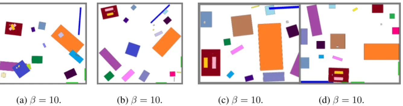
(a)β = 10. (b)β = 10. (c)β = 10. (d)β = 10.
Figure 2.9: Synthesis for different values ofβ. Each image shows a typical configuration sampled from a Markov chain.
Markov Chain Dynamics: Four types of Markov chain dynamicsqi, i = 1,2,3,4are
designed to be chosen randomly with probabilities to propose moves. Specifically, the dynamicsq1andq2 are diffusion, whileq3andq4are reversible jumps:
1. Translation of Objects. Dynamicq1 chooses a regular terminal node and samples a
new position based on the current position of the object
pos→pos+δpos, (2.27)
whereδpos follows a bivariate normal distribution.
orientation based on the current orientation of the object
θ→θ+δθ, (2.28)
whereδθfollows a normal distribution.
3. Swapping of Objects. Dynamic q3 chooses two regular terminal nodes and swaps
the positions and orientations of the objects.
4. Swapping of Supporting Objects.Dynamicq4chooses an address terminal node and
samples a new regular furniture terminal node pointed to. We sample a new 3D location(x, y, z)for the supported object:
• Randomly samplex=ux∗wp, whereux ∼unif(0,1), andwpis the width of the
supporting object.
• Randomly sampley = uy∗lp, where uy ∼ unif(0,1), andlp is the length of the
supporting object.
• The heightzis simply the height of the supporting object.
Adopting the Metropolis-Hastings algorithm, a newly proposed parse graphpg0is accepted
according to the following acceptance probability: α(pg0|pg,Θ) = min(1,p(pg 0|Θ)p(pg|pg0) p(pg|Θ)p(pg0|pg)) (2.29) = min(1,p(pg 0|Θ) p(pg|Θ)) (2.30) = min(1,exp(E(pg|Θ)− E(pg0|Θ))). (2.31)
The proposal probabilities are canceled since the proposed moves are symmetric in prob-ability.
Convergence: To test if the Markov chain has converged to the prior probability, we keep a histogram of the energy of the lastw samples. When the difference between two histograms at a distance ofssampling steps is smaller than a threshold, the Markov chain is considered to have converged.
Tidiness of Scenes: During the sampling process, a typical state is drawn from the dis-tribution. We can easily control the level of tidiness of the sampled scenes by adding an extra parameterβto control the landscape of the prior distribution:
p(pg|Θ) = 1
Z exp{−βE(pg|Θ)}. (2.32) Some examples are shown in Figure 2.9.
Note that the parameterβis analogous albeit differs from the temperature in simulated annealing optimization—the temperature in simulated annealing is time-variant; i.e., it
changes during the simulated annealing process. In our model, we simulate a Markov chain under one specificβ to get typical samples at a certain level of tidiness. When β is small, the distribution is “smooth”;i.e., the differences between local minima and local
maxima are small. A simulated annealing scheme is adopted to obtain samples with high probability as shown in Figure 2.8.
2.5.3 Scene Instantiation using 3D Object Datasets
Given a generated 3D scene layout, the 3D scene is instantiated by assembling objects into it using 3D object datasets. In this work, we incorporate both ShapeNet dataset [CFG15] and SUNCG dataset [SYZ17a] as our 3D model dataset. Scene instantiation includes five steps:
1. For each object in the scene layout, find the model has the closest the length/width ratio to the dimension specified in the scene layout.
2. Align the orientations of selected models according to the orientation specified in the scene layout.
3. Transform the models to the specified positions, and scales the models according to the generated scene layout.
4. Since we only fit the length and width in Step 1, an extra step to adjust object position along the gravity direction is needed, eliminating all the floating models and the models that penetrated into each other.
5. Add the floor, walls, and ceiling to complete the instantiated scene. 2.5.4 Scene Attribute Configurations
As we generate scenes in a forward fashion, our pipeline enables the precise customization and control of important attributes of the generated scenes. Some configurations are shown in Figure 2.11. The rendered images are determined by combinations of the following four factors:
• Illuminations, including light source positions, intensities, colors, and the number of light sources.
• Material and texture of the environment;i.e., the walls, floor and ceiling.
• Cameras, such as fisheye, panorama, and Kinect cameras, have different focal lengths and apertures, yielding dramatically different rendered images. By virtue of
physics-(a) Different categories of the scenes using default attributes of object material, the lighting condi-tions, and camera parameters. Top row: top view. Bottom row: a random view.
(b) Additional examples of two bedrooms, with corresponding depth map, surface normal, and semantic segmentation.
Figure 2.10: Qualitative results in different types of scenes.
based rendering, our pipeline can even control the F-stop and focal distance, result-ing in different depths of field.
• Different object materials and textures will have various properties, represented by roughness, metallicness, and reflectivity.
2.6
Photorealistic Scene Rendering
We adopt Physics-Based Rendering (PBR) [PH04] to generate the photorealistic 2D im-ages. PBR has become the industry standard in computer graphics applications in re-cent years, and has been widely adopted for both offline and real-time rendering. Unlike traditional rendering techniques where heuristic shaders are used to control how light is scattered by a surface, PBR simulates the physics of real-world light by computing the bidirectional scattering distribution function (BSDF) [BDW81] of the surface.
(a) Lighting intensity: half and double (b) Lighting color: purple and blue
(c) Different object materials: metal, gold, chocolate, and clay
Figure 2.11: We can configure the scene with different (a) illumination intensities, (b) illumination colors, (c) materials, and (d) even on each object part. We can also control (e) the number of light source and their positions, (f) camera lenses (e.g., fish eye), (g)
depths of field, or (h) render the scene as a panorama for virtual reality and other virtual environments. (i) 7 different background wall textures. Note how the background affects the overall illumination.
Formulation: Following the law of conservation of energy, PBR solves the rendering equation for the total spectral radiance of outgoing light in directionwfrom pointxon a surface Lo(x,w) = Le(x,w) (2.33) + Z Ω fr(x,w0,w)Li(x,w0)(−w0·n)dw0,
whereLo is the outgoing light,Le is the emitted light (from a light source),Ωis the unit
hemisphere uniquely determined by xand its normal, fr is the bidirectional reflectance