A NEW LANCZOS-TYPE ALGORITHM FOR SYSTEMS OF LINEAR EQUATIONS
MUHAMMAD FAROOQ1 AND ABDELLAH SALHI2
Abstract. Lanczos-type algorithms are efficient and easy to imple-ment. Unfortunately they breakdown frequently and well before con-vergence has been achieved. These algorithms are typically based on recurrence relations which involve formal orthogonal polynomials of low degree. In this paper, we consider a recurrence relation that has not been studied before and which involves a relatively higher degree polynomial. Interestingly, it leads to an algorithm that shows su-perior stability when compared to existing Lanczos-type algorithms. This new algorithm is derived and described. It is then compared to the best known algorithms of this type, namely A5/B10,A8/B10,
as well as Arnoldi’s algorithm, on a set of standard test problems. Numerical results are included.
Key words : Lanczos algorithm; Arnoldi algorithm; Systems of Lin-ear Equations; Formal Orthogonal Polynomials
AMS SUBJECT: Primary 65F10.
1. Introduction and background
The Lanczos algorithm, [28, 29, 14], is an iterative process that has been primarily designed to calculate the eigenvalues of a matrix. How-ever, it has found a wide application in the area of Systems of Lin-ear Equations (SLE’s) where it now is a well established solver. Its attraction resides in its efficiency as it only involves vector-to-vector and matrix-to-vector products. Moreover, in exact arithmetic, it con-verges to the exact solution in at mostn steps, wheren is the dimension
1Department of Mathematics, University of Peshawar, Khyber Pakhtunkhwa,
25120, Pakistan. Email: [email protected]
2Department of Mathematical Sciences, University of Essex, Wivenhoe Park,
Colch-ester, CO4 3SQ, UK. E-mail: [email protected].
of the problem, [29]. While efficiency is its strong point, stability is not. Indeed, it is well known to breakdown as orthogonality of the so called Lanczos vectors, generated during the solution process, is lost. Efforts to avoid this breakdown led to a flurry of papers particularly from Brezinski and his team, [2, 5, 6, 7, 10, 12, 11, 13], and others, [4, 8, 15, 17, 20, 21, 23, 24, 31, 32, 33, 35, 38, 39].
Several Lanczos-type algorithms have been designed and among them, the famous conjugate gradient algorithm of Hestenes and Stiefel, [25], when the matrix is Hermitian and the bi-conjugate gradient algorithm of Fletcher, [22], and the algorithm of Arnoldi, [1, 36], in the general case.
Lanczos-type algorithms are commonly derived from recurrence rela-tions typically using Formal Orthogonal Polynomials (FOP’s) of low de-gree, [29, 6, 16, 37]. Recurrence relations using relatively higher degree FOP’s have not been investigated. Here, we set out to design an algo-rithm that is based on such recurrence relations and FOP’s, and study its properties and, in particular, its stability.
1.1. The Lanczos Process. Consider the SLE
Ax=b, (1)
whereA∈Rn×n, b∈Rn and x∈Rn.
Let x0 and y be two arbitrary vectors in Rn such that y 6= 0 then
Lanczos method [29] consists in constructing a sequence of vectors xk∈
Rn defined as follows
xk−x0 ∈Kk(A,r0) =span(r0,Ar0, . . . ,Ak−1r0), (2)
rk =b−Axk⊥Lk(AT,y) =span(y,ATy, . . . ,AT
k−1
y), (3) whereAT denotes the transpose of A.
Equation (2) gives,
xk−x0 =−α1r0−α2Ar0− · · · −αkAk−1r0. (4)
Multiplying both sides by A and adding and subtracting b on the left hand side gives
rk =r0 +α1r0+α2Ar0+· · ·+αkAk−1r0. (5)
If we set
Pk(x) = 1 +α1x+...+αkx,
then we can write from (5)
From (3), the orthogonality condition gives (AT iy,r
k) = (y,Airk) = (y,AiPk(A)r0) = 0, for i= 0, ..., k−1.
Thus, the coefficientsα1,...,αk form a solution of SLE’s,
α1(y,Ai+1r0)+...+αk(y,Ai+kr0) =−(y,Air0), fori= 0, . . . , k−1. (7)
If the determinant of the above system is not zero then its solution exists and allows to obtainxk andrk. Obviously, in practice, solving the above
system directly for increasing values of k is not feasible; k is the order of the iterate in the solution process. We shall see now how to solve this system for increasing values ofkrecursively, that is, if polynomialsPkcan
be computed recursively. Such computation is feasible, since polynomials
Pk form a family of FOP’s which will briefly be explained below.
1.2. Formal Orthogonal Polynomials. Define a linear functional c
on the space of reel polynomials by
c(xi) =c
i for i= 0,1, . . .
where
ci = (AT iy,rk) = (y,Airk) for i= 0,1, . . .
Write the orthogonality condition as,
c(xiP
k) = 0 for i= 0, . . . , k−1. (8)
The above condition shows that Pk is the polynomial of degree at most k and is a FOP with respect to the functional c, [5]. The normalization condition for these polynomials is Pk(0) = 1; Pk exists and is unique if the following Hankel determinant
H(1)k = ¯ ¯ ¯ ¯ ¯ ¯ ¯ ¯ c1 c2 · · · ck c2 c3 · · · ck+1 ... ... ... ck ck+1 · · · c2k−1 ¯ ¯ ¯ ¯ ¯ ¯ ¯ ¯ is not zero. In that case we can writePk(x) as follows.
Pk(x) = ¯ ¯ ¯ ¯ ¯ ¯ ¯ ¯ 1 x · · · xk c0 c1 · · · ck ... ... ... ck−1 ck · · · c2k−1 ¯ ¯ ¯ ¯ ¯ ¯ ¯ ¯ ¯ ¯ ¯ ¯ ¯ ¯ c1 · · · ck ... ... ck · · · c2k−1 ¯ ¯ ¯ ¯ ¯ ¯ , (9)
where the denominator of this polynomial is H(1)k , the determinant of the system (7). We assume that ∀ k, H(1)k 6= 0 and therefore all the polynomialsPk exist for all k. If for some k, H(1)k = 0, then Pk does not
exist and breakdown occurs in the algorithm, [6, 10, 11, 13, 8].
A Lanczos-type method consists in computing Pk recursively, then rk
and finally xk such that rk = b−Axk, without inverting matrix A. In
exact arithmetic, this gives the solution of the system (1) in at most n
steps, wheren is the dimension of the SLE, [6, 12].
1.3. Notation and organization. The notation introduced by Baheux, in [2, 3], for recurrence relations with three terms is adopted here. It puts recurrence relations involving FOP’sPk(x) (the polynomials of degree at mostk with regard to the linear functional c) and/or FOP’s Pk(1)(x) (the polynomials of degree at most k with regard to linear functional c(1),
[9]) into two groups: Ai and Bj. Although relationsAi, when they exist, rarely lead to Lanczos-type algorithms on their own (the exceptions being
A4, [2, 3], andA12, [17], so far), relationsBjnever lead to such algorithms
for obvious reasons. It is the combination of recurrence relations Ai
and Bj, denoted as Ai/Bj, when both exist, that lead to Lanczos-type
algorithms. In the following we will refer to algorithms by the relation(s) that lead to them. Hence, there are, potentially, algorithms Ai and
algorithms Ai/Bj, for some i= 1,2, . . . and some j = 1,2, . . .
In this paper, a new algorithm based on a recurrence relation that has not been studied before, is derived. It is then compared to three other algorithms, one of which is the Arnoldi algorithm.
The rest of the paper is organized as follows. In the next section, the Lanczos-type algorithmA8/B10, [2], and the estimation of the
coeffi-cients of the recurrence relationsA8 and B10 used to derive it are given.
A12, [17], used to derive the new algorithm of the same name. Section
4 describes the test problems and reports numerical results. Section 5 is the conclusion and further work.
2. Baheux algorithm A8/B10
The choice of algorithm A8/B10, for comparison with our own is
dic-tated by the fact that this is the most robust of the algorithms considered in [2, 3] on some of the problems considered here. So, outperforming this algorithm implies outperforming the rest of the algorithms considered therein.
For completeness, we recall the relevant relations between adjacent FOPs that lead toA8/B10 and their coefficients estimates. These are A8
and B10. The details of algorithmA5/B10 are given in [3].
2.1. Recurrence relation A8. RelationA8 is
Pk(x) = (Akx+Bk)Pk−(1)1(x) + (Ckx+Dk)Pk−1(x), (10)
first investigated in [2, 3]. Its coefficients are estimated as
Bk = 0, (11) Ck= 0, (12) Dk= 1, (13) and Ak=−c(x k−1Pk− 1(x)) c(xkP(1) k−1(x)) . (14) As we know ( c(xkPk) = (AT ky, Pk(A)r 0) = (yk,rk), c(xkP(1) k ) = (AT ky, P (1) k (A)r0) = (yk,zk), (15) with yk = ATyk−1 and zk is defined in (21). Using (15), equation (14)
becomes Ak =−(yk−1,rk−1) (yk,zk−1) =− (yk−1,rk−1) (yk−1,Azk−1) . (16)
2.2. Recurrence relationB10. This relation, first investigated in [2, 3],
is
Pk(1)(x) = (A1kx+Bk1)Pk−(1)1(x) +Ck1Pk(x), (17) Its coefficients are estimated as
A1
k = 0, (18)
C1
kak= 1, (19)
whereak is the coefficient of xk in Pk(x) defined in (10) and B1 k=− C1 kc(yk,rk) c(yk,zk−1) . (20) Equation (17) gives zk =Bk1zk−1 +Ck1rk. (21)
2.3. Algorithm A8/B10. The pseudo-code of A8/B10, due to Baheux,
[2, 3], is as follows.
Algorithm 1AlgorithmA8/B10
Choose x0 andysuch that y6= 0, and² arbitrarily small and positive.
Set r0 =b−Ax0,
z0 =r0,
y0 =y,
for k= 0,1,2, . . ., do
Ak+1 =−(yk(yk,Azk),rk) ,
rk+1 =rk+Ak+1Azk, xk+1 =xk−Ak+1zk. if ||rk+1|| ≥², then yk+1 =ATy k, C1 k+1 = Ak1+1, B1 k+1 =− C1 k+1(yk+1,rk+1) (yk,Azk) , zk+1 =Bk1+1zk+Ck1+1rk+1. else
Stop; solution found.
end if end for
3. A new Lanczos-type algorithm
In the following, a new recurrence relation which leads to a new variant of the Lanczos algorithm is considered.
3.1. Recurrence relation A12. Consider the following recurrence
rela-tion, [17, 19]
Pk(x) = Ak[(x2+Bkx+Ck)Pk−2(x) + (Dkx3+Ekx2+Fkx+Gk)Pk−3(x)],
(22) fork ≥3, whereAk,Bk,Ck,Dk,Ek,FkandGkare constants to be deter-mined using the normalization conditionPk(0) = 1 and the orthogonality conditions c(xiPk) = 0, ∀i = 0, . . . , k −1, xi being a monic polynomial
of exact degree i. To find these coefficients, we proceed as follows. Since ∀k, Pk(0) = 1, equation (22) gives
1 = Ak[Ck+Gk].
Multiplying both sides of (22) by xi and then applying the linear
func-tionalc, we get
c(xiP
k) =Ak{c(xi+2Pk−2) +Bkc(xi+1Pk−2) +Ckc(xiPk−2) +Dkc(xi+3Pk−3)
+Ekc(xi+2Pk−3) +Fkc(xi+1Pk−3) +Gkc(xiPk−3)}.
(23) Equation (23) is always true fori= 0, ..., k−7.
Fori=k−6, we have 0 =Dkc(xk−3Pk−3). Sincec(xk−3Pk− 3)6= 0, we have Dk= 0. Fori=k−5, we get 0 =Ekc(xk−3Pk−3). But c(xk−3P k−3)6= 0; therefore Ek = 0. Fori=k−4, (23) gives Fk=− c(xk−2P k−2) c(xk−3Pk−3). (24)
For i = k−3, i = k −2 and i = k−1 we get the following equations respectively Bkc(xk−2Pk−2) +Gkc(xk−3Pk−3) =−c(xk−1Pk−2)−Fkc(xk−2Pk−3), (25) Bkc(xk−1Pk−2) +Ckc(xk−2Pk−2) +Gkc(xk−2Pk−3) =−c(xkPk− 2)−Fkc(xk−1Pk−3), (26) and Bkc(xkPk−2) +Ckc(xk−1Pk−2) +Gkc(xk−1Pk−3) =−c(xk+1P k−2)−Fkc(xkPk−3). (27)
Leta11,a12,a13,a21,a22,a23,a31,a32, anda33be the coefficients ofBk, Ck andGkin equations (25), (26) and (27) respectively and letb1,b2 and
b3 be the corresponding right sides of these equations. If ∆k represents
the determinant of the coefficients matrix of the above mentioned system of equations then, we have
a11=c(xk−2Pk−2), a12 = 0, a13=c(xk−3Pk−3), a21=c(xk−1Pk−2), a22 =c(xk−2Pk−2),a23=c(xk−2Pk−3), a31=c(xkPk−2), a32=c(xk−1Pk−2),a33 =c(xk−1Pk−3), b1 =−c(xk−1Pk−2)−Fkc(xk−2Pk−3) =−a21−Fka23, b2 =−c(xkPk−2)−Fkc(xk−1Pk−3) = −a31−Fka33, b3 = −c(xk+1Pk−2)−Fkc(xkPk−3) = −s−Fkt, where s = c(xk+1Pk−2) and t=c(xkP k−3).
Therefore, equations (25), (26) and (27) can be written as
a11Bk+ 0Ck+a13Gk =b1, (28)
a21Bk+a22Ck+a23Gk=b2, (29)
a31Bk+a32Ck+a33Gk=b3. (30)
To solve forBk, Ck and Gk, Cramer’s rule requires
∆k=a11(a22a33−a32a23) +a13(a21a32−a31a22). If ∆k6= 0, then Bk = b1(a22a33−a32a23) +a13(b2a32−b3a22) ∆k , (31) Gk = b1−a11Bk a13 , (32) Ck = b2−a21Bk−a23Gk a22 , (33)
and
1 = Ak[Ck+Gk]. (34)
With all the necessary coefficients now determined, the expression of the polynomials Pk(x) becomes
Pk(x) =Ak{(x2+Bkx+Ck)Pk−2(x) + (Fkx+Gk)Pk−3(x)}. (35)
Let us now use the relation (35) to computePk(x), necessary for the com-putation of the residual rk=b−Axk =Pk(A)r0 and the corresponding
vectorxk.
Assume that Pk has exact degree k and the 3-term recurrence
rela-tionship (35) holds. To move to the Krylov space, replace x by A and multiply both side of (35) byr0 to get,
Pk(A)r0 =Ak[(A2+BkA+CkI)Pk−2(A)r0+(FkA+GkI)Pk−3(A)r0]. (36)
Using equation (6), gives
rk=Ak{(A2+BkA+CkI)rk−2+ (FkA+GkI)rk−3}. (37)
And usingrk =b−Axk, gives
xk=Ak{Ckxk−2+Gkxk−3−(Ark−2+Bkrk−2+Fkrk−3)}, (38)
with Fk as in equation (24). Using (15),Fk can be written as
Fk=−
(yk−2,rk−2)
(yk−3,rk−3)
.
Condition (15) can be used equally to rewrite the expressions of a11,
through a33,b1 tob3 as follows. a11= (yk−2,rk−2), a12 = 0, a13= (yk−3,rk−3), a21= (yk−1,rk−2), a22 = (yk−2,rk−2),a23 = (yk−2,rk−3), a31= (yk,rk−2), a32= (yk−1,rk−2), a33 = (yk−1,rk−3), b1 =−a21−Fka23, b2 =−a31−Fka33, b3 =−s−Fkt, wheres = (yk+1,rk−2) andt = (yk,rk−3).
These parameters allow the explicit computation of Bk, Gk, Ck, and Ak
as is given by equations 31, 32, 33 and 34 respectively. Equations (37) and (38) define the new Lanczos-type algorithm.
Now, since all previous formulae are only valid fork ≥3, it is necessary to find the expressions of the polynomials of degrees 1 and 2. From (9), we can write P1(x) = ¯ ¯ ¯ ¯ c10 cx1 ¯ ¯ ¯ ¯ c1 , P1(x) = 1− c0 c1 x, r1 =r0− cc10Ar0, andx1 =x0+ cc01r0, whereci = (y,Air0).
Using (9) again, we can write
P2(x) = ¯ ¯ ¯ ¯ ¯ ¯ 1 x x2 c0 c1 c2 c1 c2 c3 ¯ ¯ ¯ ¯ ¯ ¯ ¯ ¯ ¯ ¯ cc12 cc23 ¯ ¯ ¯ ¯ , P2(x) = 1− c0c3−c1c2 c1c3−c22 x+c0c2−c 2 1 c1c3−c22 x2, r2 =r0−αAr0+βA2r0, andx2 =x0+αr0−βAr0, where α= c0c3−cδ 1c2, β = c0c2−c21 δ and δ=c1c3−c22.
3.2. Algorithm A12. Putting together the various steps given in the
Algorithm 2AlgorithmA12
Choose x0 and y such that y6= 0, and choose ² arbitrarily small and
positive. Set r0 =b−Ax0, y0 =y, p=Ar0, p1 =Ap, c0 = (y,r0), c1 = (y,p), c2 = (y,p1), c3 = (y, Ap1), δ=c1c3−c22, α= c0c3−c1c2 δ , β = c0c2−c21 δ , r1 =r0− cc01p, x1 =x0+cc01r0, r2 =r0−αp+βp1, x2 =x0+αr0−βp, y1 =ATy 0, y2 =ATy1, y3 =ATy2, k = 3. while ||rk|| ≥² do yk+1 =ATy k, q1 =Ark−1,q2 =Aq1,q3 =Ark−2, a11= (yk−2,rk−2), a13 = (yk−3,rk−3),a21 = (yk−1,rk−2),a22=a11, a23= (yk−2,rk−3), a31 = (yk,rk−2), a32 =a21, a33= (yk−1,rk−3), s= (yk+1,rk−2), t= (yk,rk−3),Fk=−aa1113, b1 =−a21−a23Fk, b2 =−a31−a33Fk, b3 =−s−tFk, ∆k =a11(a22a33−a32a23) +a13(a21a32−a31a22), Bk = b1(a22a33−a32a23∆k)+a13(b2a32−b3a22), Gk= b1−a11Bk a13 , Ck = b2−a21Ba22k−a23Gk, Ak = Ck+1Gk, rk =Ak{q2+Bkq1+Ckrk−2+Fkq3+Gkrk−3}, xk =Ak{Ckxk−2+Gkxk−3−(q1+Bkrk−2+Fkrk−3)}, k=k+ 1. end while
Stop; solution found.
4. Numerical results
A12, [17], the algorithm described in the above section, has been tested
against algorithmsA5/B10 andA8/B10, the best algorithms according to
[3, 2], as well as against the established Arnoldi algorithm, [1, 36]. 4.1. Test problems I. The test problems considered here arise in the 5-point discretisation of the operator −d2
dx2− d 2
dy2+γdxd on a rectangular region. Comparative results on instances of the following problem ranging from dimension 10 to 100 for parameterδtaking values 0.0 and 0.2 respectively, are recorded in Table 1 and Table 2.
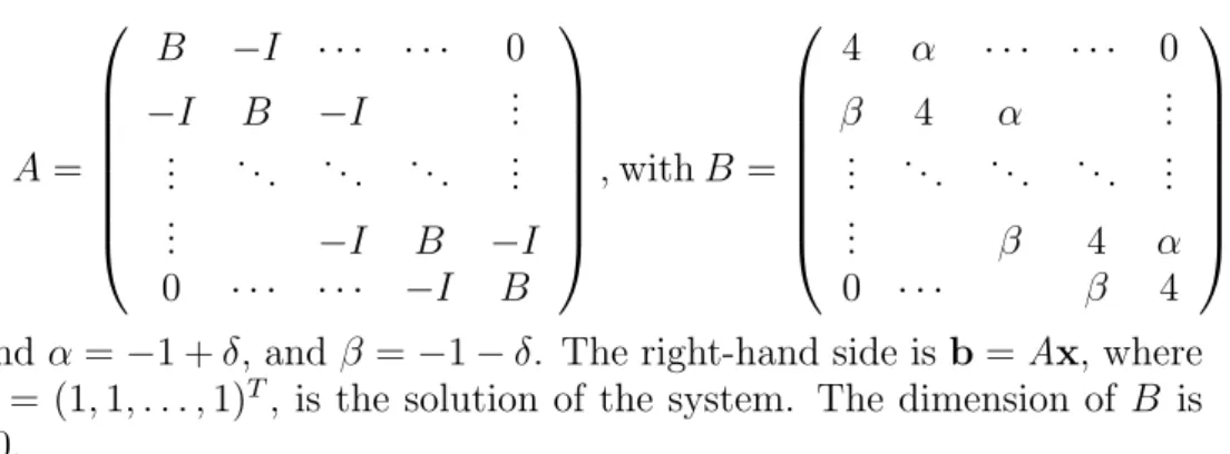
A= B −I · · · · 0 −I B −I ... ... ... ... ... ... ... −I B −I 0 · · · −I B ,withB = 4 α · · · · 0 β 4 α ... ... ... ... ... ... ... β 4 α 0 · · · β 4 .
and α=−1 +δ, and β =−1−δ. The right-hand side is b =Ax, where
x= (1,1, . . . ,1)T, is the solution of the system. The dimension of B is
10.
Table 1. Experimental results for problems when δ = 0
Arnoldi A5/B10 A8/B10 A12
n ||rk|| t(sec) ||rk|| t(sec) ||rk|| t(sec) ||rk|| t(sec)
10 1.2514E−10 0.001450 2.2940E−13 0.001892 1.7704E−13 0.002770 4.9623E−13 0.002819 20 1.7733E−11 0.002207 2.5256E−14 0.001842 1.7489E−13 0.002654 1.7536E−13 0.002904 30 1.2990E−14 0.003602 3.9026E−09 0.002220 4.9472E−09 0.003179 5.4705E−08 0.003370 40 3.5434E−11 0.006071 1.4770E−10 0.002416 8.4658E−10 0.003095 1.4776E−08 0.003526 50 6.1827E−08 0.008870 1.9959E−06 0.002962 1.3598E−06 0.003696 4.7994E−06 0.003980 60 2.9843E−14 0.012282 9.1910E−06 0.003001 3.7470E−06 0.003776 5.0010E−06 0.004354 70 4.2642E−13 0.017151 4.9035E−06 0.003622 4.2579E−06 0.004194 1.3781E−06 0.005658 80 5.0951E−08 0.021938 4.4311E−06 0.004498 7.7199E−06 0.005504 7.5581E−06 0.005271 90 9.6960E−13 0.029083 NaN 8.5560E−06 0.007900 3.7301E−06 0.006541 100 1.1397E−13 0.036462 1.1889E−06 0.003849 3.1695E−06 0.004499 8.9530E−07 0.005084
Table 2. Experimental results for problems when δ = 0.2
Arnoldi A5/B10 A8/B10 A12
n ||rk|| t(sec) ||rk|| t(sec) ||rk|| t(sec) ||rk|| t(sec)
10 2.3499E−15 0.001377 5.2347E−04 0.002339 5.2347E−04 0.002948 5.2347E−04 0.003231 20 5.6622E−11 0.002149 4.1778E−11 0.001842 5.8526E−11 0.003090 6.3915E−10 0.003372 30 6.8771E−15 0.003573 8.9881E−04 0.002220 8.9880E−04 0.003580 8.9880E−04 0.003847 40 1.8106E−10 0.006137 8.7583E−04 0.002830 9.3988E−04 0.003620 9.1261E−04 0.003977 50 3.5345E−08 0.008552 6.2669E−04 0.003360 5.7269E−04 0.004055 2.5040E−04 0.004964 60 2.8757E−13 0.012544 6.3670E−04 0.003877 8.4915E−04 0.004885 7.3489E−04 0.005345 70 4.2552E−13 0.017352 8.5670E−04 0.003902 7.0703E−04 0.006158 9.9086E−04 0.005052 80 1.7785E−04 0.021629 NaN NaN 6.5602E−04 0.012131 90 1.4837E−04 0.029332 NaN 7.5451E−04 0.011230 9.5294E−04 0.011842 100 5.8942E−13 0.037067 NaN NaN 9.9710E−04 0.018899
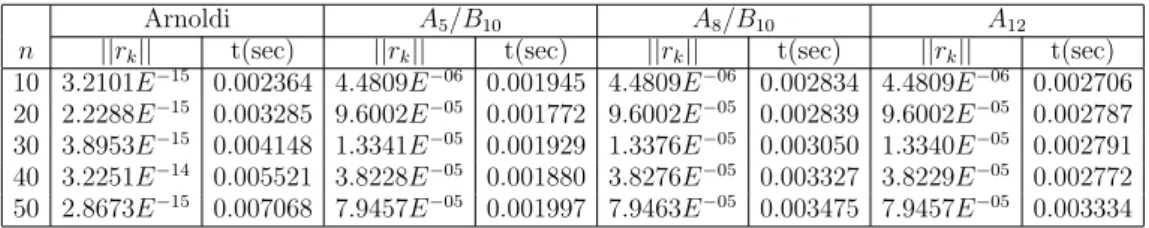
4.2. Test problems II. The coefficient matrix here is taken as the Hilbert matrix, i.e. A = hilb(n), where hilb(n) is a Matlab function,
n being the dimension of A. The right-hand side b and the solution x, are defined in the same way as in test problems I. The Hilbert matrix is notoriously ill-conditioned. Ill-conditioned systems of linear equations are notoriously difficult to solve to any useful accuracy, [18, 27, 34]
Table 3. Experimental results when A is a Hilbert matrix.
Arnoldi A5/B10 A8/B10 A12
n ||rk|| t(sec) ||rk|| t(sec) ||rk|| t(sec) ||rk|| t(sec)
10 3.2101E−15 0.002364 4.4809E−06 0.001945 4.4809E−06 0.002834 4.4809E−06 0.002706 20 2.2288E−15 0.003285 9.6002E−05 0.001772 9.6002E−05 0.002839 9.6002E−05 0.002787 30 3.8953E−15 0.004148 1.3341E−05 0.001929 1.3376E−05 0.003050 1.3340E−05 0.002791 40 3.2251E−14 0.005521 3.8228E−05 0.001880 3.8276E−05 0.003327 3.8229E−05 0.002772 50 2.8673E−15 0.007068 7.9457E−05 0.001997 7.9463E−05 0.003475 7.9457E−05 0.003334
All algorithms have been implemented in Matlab version 7.8.0 and run on a PC, under Microsoft Windows XP Professional Operating Sys-tem, with 3.2GB RAM, and 2.40 GHz Intel(R) Core(TM) 2 CPU 6600. The problems are solved as dense problems, i.e. no sparsity has been exploited. The results point to the Arnoldi algorithm being the most ro-bust overall, but also the slowest overall. AlgorithmsA5/B10andA8/B10
are the fastest overall, but the least robust overall; in fact they have failed to solve some problems in high dimension due to breakdown, of course, which is endemic in Lanczos-type algorithms. Algorithm A12,
like Arnoldi, solved all problems but faster and not as accurately. It is also more robust thanA5/B10 andA8/B10 overall, but slower than both
of them overall. Its lower speed compared to that ofA5/B10 andA8/B10
is expected since the recurrence relation A12 involves more coefficients
than both recurrence relations A5/B10 and A8/B10. Note that on the
Hilbert-type problems, Table 3, the algorithms could not cope with di-mensions higher than 50. Arnoldi is again the most stable overall and the slowest as the dimension grows. The other three algorithms have similar performances.
5. Conclusion and further work
The way Lanczos-type algorithms are derived using recurrence rela-tions involving FOP’s means that many such algorithms can be created, each based on a different set of relations. The choice of recurrence re-lations to use is dictated by the degree of FOP’s to be involved; high degrees mean a large number of coefficients have to be calculated in the
concerned Lanczos process. This, consequently, dictates the computa-tional complexity of the resulting Lanczos-type algorithm. However, it is well known, [26, 30], that computational complexity does not always imply efficiency, or indeed robustness. Moreover, robustness and accu-racy are often more important. It is therefore worthwhile to look beyond complexity issues sometimes, like we did here.
In this paper we have shown that, indeed, there are recurrence rela-tions worth exploring since they lead to more robust algorithms. As a result, a new Lanczos-type algorithm, A12 has been designed. The
nu-merical performance of this algorithm is compared to that of two existing Lanczos-type algorithms, which were found to be the best among a num-ber of Lanczos-type algorithms, [2, 3], on the same set of problems as considered here. It is also compared to the well established Arnoldi algo-rithm. It is interesting to find that algorithmA12 is overall more robust
thanA5/B10andA8/B10and faster than Arnoldi’s. This makes it occupy,
at least on the set of problems used here and elsewhere, a happy medium position. It is therefore the ideal candidate for time-limited applications which do not require high accuracy.
References
[1] W. E. Arnoldi. The principal of minimized iterations in the solution of the matrix eigenvalue problem.Quarterly of Applied Mathematics, 9 (1951):17–29.
[2] C. Baheux. New Implementations of Lanczos Method.Journal of Computational and Applied Mathematics, 57 (1995):3–15.
[3] C. Baheux.Algorithmes d’implementation de la m´ethode de Lanczos. PhD thesis, University of Lille 1, France, 1994.
[4] A. Bjˆorck, T. Elfving, and Z. Strakos. Stability of Conjugate Gradient and Lanc-zos Methods for Linear Least Squares Problems.SIAM Journal of Matrix Anal-ysis and Application, 19 (1998):720–736.
[5] C. Brezinski. Pad´e-Type Approximation and General Orthogonal Polynomials, Internat. Ser. Nuner. Math. 50. Birkh¨auser, Basel, 1980.
[6] C. Brezinski and H. Sadok. Lanczos-type algorithms for solving systems of linear equations.Applied Numerical Mathematics, 11 (1993):443–473.
[7] C. Brezinski and M. R. Zaglia. Hybird procedures for solving linear systems.
Numerische Mathematik, 67 (1994):1–19.
[8] C. Brezinski and M. R. Zaglia. A New Presentation of Orthogonal Polynomials with Applications to their Computation. Numerical Algorithms, 1 (1991):207– 222.
[9] C. Brezinski, M. R. Zaglia, and H. Sadok. Avoiding breakdown and near-breakdown in Lanczos type algorithms.Numerical Algorithms, 1 (1991):261–284. [10] C. Brezinski, M. R. Zaglia, and H. Sadok. A Breakdown-free Lanczos type
[11] C. Brezinski, M. R. Zaglia, and H. Sadok. The matrix and polynomial approaches to Lanczos-type algorithms.Journal of Computational and Applied Mathematics, 123 (2000):241–260.
[12] C. Brezinski, M. R. Zaglia, and H. Sadok. New look-ahead Lanczos-type algo-rithms for linear systems. Numerische Mathematik, 83 (1999):53–85.
[13] C. Brezinski, M. R. Zaglia, and H. Sadok. A review of formal orthogonality in Lanczos-based methods.Journal of Computational and Applied Mathematics, 140 (2002):81–98.
[14] C. G. Broyden and M. T. Vespucci.Krylov Solvers For Linear Algebraic Systems. Elsevier, Amsterdam, The Netherlands, 2004.
[15] D. Calvetti, L. Reichel, F. Sgallari, and G. Spaletta. A Regularizing Lanczos iteration method for underdetermined linear systems. Jouranl of Computational and Applied Mathematics, 115 (2000):101–120.
[16] A. Draux. Polynˆomes Orthogonaux Formels. Application, LNM 974. Springer-Verlag, Berlin, 1983.
[17] M. Farooq. New Lanczos-type Algorithms and their Implementation. PhD the-sis, University of Essex, UK, 2011. http://serlib0.essex.ac.uk/record= b1754556.
[18] M. Farooq and A. Salhi. Improving the solvability of ill-conditioned systems of linear equations by reducing the condition number of their matrices. J. Korean Math. Soc., 48 (5) (2011):939–952. http://dx.doi.org/10.4134/JKMS.2011.48.5.939.
[19] M. Farooq and A. Salhi. New Recurrence Relationships Between Orthogonal Polynomials Which Lead to New Lanczos-type Algo-rithms. Journal of Prime Research in Mathematics, 8 (2012):61–75. http://www.sms.edu.pk/journals/jprm/jprmvol8/09.pdf.
[20] M. Farooq and A. Salhi. A Preemptive Restarting Approach to Beating the Inherent Instability of Lanczos-type Algorithms. Iranian Journal of Sceince and Technology, Transaction A: Science, 37 (3.1) (2013):349–358. http://ijsts. shirazu.ac.ir/?_action=articleInfo&article=1634&vol=142.
[21] M. Farooq and A. Salhi. A Switching Approach to Avoid Breakdown in Lanczos-type Algorithms. Applied Mathematics and Information Sciences, 8 (5) (2014):2161–2169.http://naturalspublishing.com/ContIss.asp?IssID= 190.
[22] R. Fletcher. Conjugate gradient methods for indefinite systems. In G.Alistair Watson, editor,Numerical Analysis, volume 506 ofLecture Notes in Mathematics, pages 73–89. Springer Berlin Heidelberg, 1976.
[23] A. Greenbaum.Iterative Methods for Solving Linear System. Society for Indus-trial and Applied Mathematics, Philadelphia, 1997.
[24] A. El Guennouni. A unified approach to some strategies for the treatment of breakdown in Lanczos-type algorithms. Applicationes Mathematicae, 26 (1999):477–488.
[25] M.R. Hestenes and E. Stiefel. Mehtods of conjugate gradients for solving linear systems.Journal of the National Bureau of Standards, 49 (1952):409–436.
[26] L. G. Khachyan. A polynomial algorithm in linear programming.Soviet Mathe-matics Doklady (translated), 20 (1979):191–194.
[27] H. J. Kim, K. Choi, H. B. Lee, H. K. Jung, and S. Y. Hahn. A new algorithm for solving ill-conditioned linear system.IEEE Transactions on Magnetics, 32(3) (1996):1373–1376.
[28] C. Lanczos. An Iteration Method for the Solution of the Eigenvalue Problem of Linear Differential and Integeral Operators.Journal of Research of the National Bureau of Standards, 45 (1950):255–282.
[29] C. Lanczos. Solution of systems of linear equations by minimized iteration. Jour-nal of the NatioJour-nal Bureau of Standards, 49 (1952):33–53.
[30] L. Lovasz. The Ellipsoid Algorithm: Better or Worse than the Simplex? Mathe-matical Intelligencer, 2 (1980):141–146.
[31] G. Meurant. The Lanczos and conjugate gradient algorithms, From Theory to Finite Precision Computations. SIAM, Philadelphia, 2006.
[32] B. N. Parlett and D. S. Scott. The Lanczos Algorithm With Selective Orthogo-naliztion.Mathematics of Computation, 33 (1979):217–238.
[33] B. N. Parlett, D. R. Taylor, and Z. A. Liu. A Look-Ahead Lanczos Algorithm for Unsymmetric Matrices. Mathematics of Computation, 44 (1985):105–124. [34] J. R. Rice.Matrix Computations and Mathematical Software. McGraw-Hill, New
York, 1981.
[35] Y. Saad. On the Lanczos method for solving linear system with several right-hand sides.Mathematics of Computation, 48 (1987):651–662.
[36] Y. Saad.Iterative methods for sparse linear systems. SIAM, Philadelphia, 2003. [37] G. Szeg¨o.Orthogonal Polynomials. American Mathematical Society, Providence,
Rhode Island, 1939.
[38] H. A. Van der Vorst. An iterative solution method for solving f(A)x=b, using Krylov subspace information obtained for the symmetric positive definite matrix A. Journal of Computational and Applied Mathematics, 18(2) (1987):249–263. [39] Q. Ye. A Breakdown-Free Variation of the Nonsymmetric Lanczos Algorithms.