Panel time series analysis : some theory and applications

(1)

Panel Time Series Analysis: Some Theory

and Applications

Andrea Nocera

Department of Economics, Mathematics and Statistics

Birkbeck, University of London

A thesis submitted for the degree of

Doctor of Philosophy

(2)

Declaration

I wish to declare that no part of this doctoral dissertation contains material previously submitted to the University of London or to any other institution for any degree. The fourth chapter of this thesis, titled “ House Prices and Monetary Policy in the Euro Area: Evidence from Structural VARs”, is a joint work with Mr. Moreno Roma. I certify that I am the lead author of the research, having designed and carried out the empirical analysis, which constitutes the bulk of the chapter.

Andrea Nocera

London, United Kingdom

28 June 2017

(3)

Abstract

This thesis offers some theoretical contributions to the literature on large hetero-geneous panel data models. It also demonstrates their practical use in empirical research, in the field of housing in macroeconomics, and for the analysis of the determinants of sovereign credit spreads.

The first chapter provides the motivation for the research presented in this thesis.

In the second chapter, we investigate the causes and the finite-sample con-sequences of negative definite covariance matrices in Swamy type random coef-ficient models. Monte Carlo experiments reveal that the negative definiteness problem is less severe when the degree of coefficient dispersion is substantial, and the precision of the regression disturbances is high. The sample size also plays a crucial role. We then evaluate the direct consequences of relying on the asymptotic properties of the estimator of the random coefficient covariance for hypothesis tests.

A solution to the aforementioned problem is proposed in the third chapter. In particular, we propose to implement the EM algorithm to compute restricted maximum likelihood estimates of both the average effects and the unit-specific coefficients as well as of the variance components in a wide class of heterogen-eous panel data models. Compared to existing methods, our approach leads to unbiased and more efficient estimation of the variance components of the model without running into the problem of negative definite covariance matrices typic-ally encountered in random coefficient models. This in turn leads to more accurate

(4)

4

estimated standard errors and hypothesis tests. Monte Carlo simulations reveal that the proposed estimator has relatively good finite sample properties. In eval-uating the merits of our estimator, we also provide an overview of the sampling and Bayesian methods commonly used to estimate heterogeneous panel data. A novel approach to investigate heterogeneity of the sensitivity of sovereign spreads to government debt is presented.

In a final chapter, we use a structural Bayesian (stochastic search variable selection) vector autoregressive model to investigate the heterogeneous impact of housing demand shocks on the macro-economy and the role of house prices in the monetary policy transmission, across euro area countries. A novel set of identi-fication restrictions, which combines zero and sign restrictions, is proposed. By exploiting the cross-sectional dimension of our data, we explore the differences in the propagation channels of house prices and monetary policy and the chal-lenges they pose in the process of real and nominal convergence in the Eurozone. Among the main results, we find a comparatively stronger housing wealth effect on consumption in Ireland and Spain. We provide new evidence in support of the financial accelerator hypothesis, showing that house prices play an important role in the availability of loans. A significant and highly heterogeneous effect of monetary policy on house price dynamics is also documented.

(5)

Acknowledgements

My adventure at Birkbeck started in September 2012. Willing to expand my knowledge of econometrics, I enrolled to a postgraduate degree on that topic. It was there that I had the great pleasure of meeting Haris Psaradakis, who was to become my PhD supervisor at the same institution, the year after. I consider myself very fortunate. I am very grateful to him for his encouragements and his constant help, above and beyond the call of duty. I have also been very lucky to have Ron Smith as supervisor. I have truly enjoyed our discussions on panel data and not only; seeing his office door open has always been an irresistible temptation. His guidance has proved extremely helpful. I wish one day to be as helpful and inspiring to the future generations as Haris and Ron were to me.

Ivan Petrella has also played an important role during my years at Birkbeck. I would like to sincerely thank him for his sharing his passion for research, and for his numerous and invaluable advices throughout the years. Completing a PhD thesis can be a long process, during which it is inevitable to encounter many exceptional people. A big thank to the PhD students, Adiya, Angelos, Lasse, Marco, José, Paul, Rubens, and many others, with whom I have shared hope and “despair”, and to all members of the staff in our Department.

Recently, I had the pleasure of visiting the USC Dornsife INET, in Los Angeles. I am very grateful to Hashem Pesaran for the kind and warm hos-pitality received. I feel honoured to have the opportunity to join his centre, as postdoctoral research fellow, and I can’t wait to start. Part of the fourth chapter has been written during my traineeship at the European Central Bank, Prices

(6)

6

and Costs Division. I would like to thank the staff members for their warm hos-pitality. I would also like to thank George Kapetanios and Takashi Yamagata for kindly accepting to examine this thesis. Financial support from the Economic and Social Research Council is gratefully acknowledged.

Any occasion is a good one to thank all my dear friends, Anastasia, Andrea, Dimitri, Doriana, Giovanni and Giovanni, Grzegorz, Ido, and Marco, among oth-ers.

Finally, I would like to express my strong appreciation to my parents, Alfonso and Ninetta, for their unconditional and constant love and support. Dulcis in fundo, my dearest Natalia. Everything becomes much easier with her by my side.

(7)

List of Figures

2.1 Rejection Frequency for Slope Parameter . . . 44

2.2 Rejection Frequency for Intercept Parameter . . . 45

3.1 Bias and RMSE of Average Effects . . . 84

3.2 Bias and RMSE of Variance Components . . . 85

3.3 Power Functions . . . 86

3.4 Bias and RMSE of Bayes Estimator of Average Effects . . . 88

3.5 Bias and RMSE of Bayes Estimator of Variance Components . . . 89

4.1 Selected Impulse Response to a Housing Demand Shocks . . . 136

4.2 Impulse Response of Real Loans to a Housing Demand Shock . . 137

4.3 Impulse Response of Real Private Consumption to a Housing De-mand Shock . . . 138

4.4 Forecast Error Variance of Selected Variables Accounted by Innov-ations in Real House Prices . . . 139

4.5 Impulse Response of House Prices to a Monetary Policy Shock . . 140

4.6 Impulse Response of Real Loans to a Monetary Policy Shock . . . 141

4.7 Forecast Error Variance of Selected Variables Accounted by Innov-ations in Monetary Rate . . . 142

4.8 Historical Counterfactuals for Real Private Consumption . . . 144

4.9 Historical Counterfactuals for Real Loans . . . 146

4.10 Historical Counterfactuals for Real House Prices . . . 147

(12)

List of Figures 12

(13)

List of Tables

2.1 The probability of 4ˆ being negative definite . . . 33

2.2 The drivers of the random coefficient covariance’s negative defin-iteness problem . . . 36

2.3 Bias and root mean square errors of4ˆ1 . . . 38

2.4 Accuracy of estimated standard errors . . . 40

2.5 Empirical moments of F-statistics . . . 42

2.6 Empirical sizes based on F-statistics . . . 43

3.1 Determinants of sensitivity of spreads: EM-REML Estimates. . . 94

3.2 Determinants of sensitivity of spreads to government debt: EM-REML Estimates. . . 97

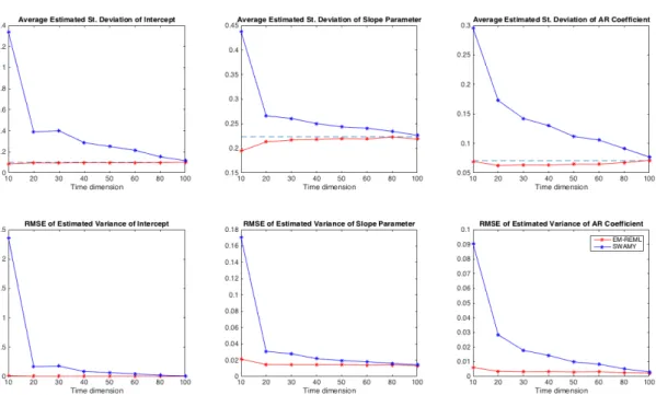
3.3 Properties of EM-REML estimator as T gets large, for fixed N . . 100

3.4 Properties of Swamy estimator as T gets large, for fixed N . . . . 101

3.5 Properties of Mean Group estimator asT gets large, for fixed N . 102 4.1 Selected Empirical Evidence . . . 127

4.2 Short Run Responses to Housing Demand and Monetary Policy Shocks . . . 131

(14)

Chapter 1 Introduction

1.1 Motivation and Contributions

Panel data models have become increasingly popular in empirical studies. In fact, by combining a number of observations on a cross-section of units (individuals, countries, or firms, to name a few) over repeated time periods, they provide a number of advantages over a single cross-section, or a single time series. Hsiao (2003) and Baltagi (2005) offer a comprehensive list of benefits from using panel data. Among them, the availability of larger data sets which increases the degrees of freedom, may alleviate multicollinearity and hence improve efficiency, and the ability to study dynamics of adjustment. Another important advantage, to which we pay particular attention in this thesis, is the ability to control for individual heterogeneity. A notable example is Baltagi and Levin (1992). They study cigar-ette demand across 46 American states by modelling consumption as a function of its own lag, price and income. They note that panel data are able to control for state-invariant (e.g. advertising on TV) and time-invariant variables (such as religion), even though some of them may not be available or measurable. This in turn avoids the omission bias in the resulting estimates.

Traditionally, in panel data with large number of cross-section units (N) and few time periods (T), the effects of unobserved time-invariant heterogeneity and

(15)

1.1. Motivation and Contributions 15

omitted variables have been controlled by allowing for individual-specific inter-cepts and/or time-specific effects. However, in many economic applications, it is unlikely that the response of a dependent variable to a change in an explanatory variable is the same for all units and/or over time. AsT increases, it is possible to test for equality of parameters, and the homogeneity hypothesis is often rejected in practice.1 _{Accounting for heterogeneity may help to shed new lights and to}

bet-ter understanding some real economic phenomena. For instance, Eberhardt and Teal (2010) emphasize the importance of parameter heterogeneity in the growth empiric literature. Haque, Pesaran and Sharma (2000) investigate the implica-tions of neglected slope heterogeneity for the fixed effects estimator. Focusing on cross-country savings regressions, the authors find that ignoring differences across countries can lead to overestimating the influence of certain factors on the private savings rates. At the same time, one can obtain highly significant, but spurious, nonlinear effects for some of the potential determinants, although the country-specific regressions are linear.

The treatment of heterogeneity is particularly important in the context of dynamic models. Pesaran and Smith (1995) show that when the regression coef-ficients vary across individuals, pooling and aggregating in a dynamic model give inconsistent and misleading estimates of the coefficients. The inconsistency of both fixed and random effects does not disappear even when bothT andN go to infinity. Therefore, they argue in favour of heterogeneous estimators and propose the so called Mean Group estimation which yields a consistent estimator of the average effects as both T and N gets large.

Another popular approach which allows for coefficient heterogeneity is the Swamy (1970) random coefficient model. It can be seen as a generalization of the random effects model, since it considers both the intercept and the slope parameters as realizations from a certain probability distribution with common

1_{Different tests for slope homogeneity have been proposed. See for instance, Pesaran and}

(16)

mean and constant variance-covariance matrix. In view of this assumption, it is quite natural to put the random coefficient model in a Bayesian framework. Bayesian estimation is discussed in Maddala, Trost, Li and Joutz (1997), and Hsiao, Pesaran and Tahmiscioglu (1999), among others.

The above mentioned techniques can be labelled as large heterogeneous panel data models. Excellent surveys are provided by Hsiao and Pesaran (2008), Pesaran (2016), and Smith and Fuertes (2016). This thesis offers some theor-etical contributions to this literature. It also contains two novel applications in the context of heterogeneous panels.

First, we study the problem of negative definite covariance matrices in Swamy-type random coefficient models. As in the error-component model, the unbiased estimator of the random coefficient covariance matrix proposed by Swamy (1970) is not necessarily nonnegative definite. This is often the case in empirical applic-ations. Despite being a well acknowledged problem, its causes are not yet fully understood. We perform a Monte Carlo study to address this issue. We show that the problem is particularly severe when the precision of the regression disturb-ances and the degree of coefficient heterogeneity are low, and/or when the sample size is small. To overcome the negative definiteness problem, Swamy (1971) sug-gests an alternative estimator of the random coefficient covariance matrix which, although biased, is nonnegative definite and is consistent when the time dimen-sion tends to infinity. We demonstrate that relying on the asymptotic properties of this estimator may lead to poor inference. Unless the time and cross-section dimensions, and/or the degree of coefficient dispersion are high, the estimated standard errors are largely upwards biased. The resulting hypothesis tests may suffer from considerable size distortions. The empirical sizes of the tests are substantially lower than the nominal levels.

A solution to the aforementioned problems is provided in a separate chapter. We show that applying the EM algorithm to obtain restricted maximum likelihood estimates yields an unbiased and more efficient estimator of the random coefficient

(17)

covariance matrix without running into the problem of negative definiteness. This in turn leads to more accurate standard errors and hypothesis tests. It is also demonstrated that direct maximization of the likelihood which incorporates the prior likelihood of the random coefficients yields an estimator of the coefficients’ covariance matrix which does not satisfy the law of total variance. This is not the case when employing the EM algorithm.

Since the seminal work of Dempster, Laird, and Rubin (1977), the EM al-gorithm has been successfully applied in different contexts, such as linear mixed models (Laird and Ware, 1982), finite mixture models (McLachlanand Peel, 2000), and factor analysis (Engle and Watson, (1983), Quah and Sargent (1993), Doz, Giannone, and Reichlin (2012), Harvey and Liu (2016)), to mention a few. A full-fledged book on the subject is McLachlan and Krishnan (2008). We highlight the relative merits of the EM approach in estimating both average and unit-specific coefficients in heterogeneous panels. In doing so, we also review the existing sampling and Bayesian methods. To extend the applicability of our method, we consider a general framework which incorporates various panel data models as special case, including the random coefficient and the correlated random effects models. Monte Carlo simulations reveal that the obtained (restricted) maximum likelihood estimators have relatively good finite sample properties, in terms of bias, root mean square errors, and power of tests.

An important issue in large panels, which has received particular attention in recent years, is cross-section dependence, i.e. the correlation between errors in different units. The literature is quite vast (see for instance, Holly, Pesaran, and Yamagata (2010), Chudik and Pesaran (2013), Bailey, Kapetanios and Pesaran (2015)) and its analysis is beyond the scope of this thesis. We simply note that our estimation procedure can be adapted to allow for cross-section dependence, following Pesaran (2006), and Chudik and Pesaran (2015).

The methods described above can be quite effective in modelling complex eco-nomic relationships. Therefore, part of this thesis is devoted to their application

(18)

to the analysis of sovereign credit risk and to the role of house price dynamics in the macroeconomy.

In the first application, we show that modelling the random coefficients as a function of selected explanatory variables can be beneficial to the study of the determinants of the sensitivity of sovereign spreads with respect to government debt. It is widely known that macroeconomic fundamentals and volatility are significant drivers of sovereign credit spreads (Akitoby and Stratmann (2008), Hilscher and Nosbusch (2010), among others). On the contrary, there is no study, to the best of our knowledge, which investigates why the response of sovereign spreads to changes in government debt differs significantly across countries. We show that country-specific macroeconomic indicators do not have any significant impact on the sensitivity of spreads to debt. On the other hand, history of repayment plays an important role. A 1% increase in the percentage of years in default or restructuring domestic debt is associated with around 0.35% increase in the additional risk premium in response to an increase in debt.

Another important aspect in applied research in economics is the aggregation problem. The implications of aggregation are well known in the econometrics lit-erature (e.g. Granger (1987), Pesaran (2003), and Pesaran and Chudik (2014)). Nevertheless, some of the issues which arise when aggregating time series are sometimes ignored in the applied literature. For example, most of the recent studies which derive insights on the role of the housing market in the Eurozone from multivariate structural models focus on the euro area as a whole. A prom-inent example is Musso, Neri, and Stracca (2011). However, it is important from a policy perspective to quantify and compare the heterogeneous impacts of house prices across countries as they can amplify the existing economic divergences across Eurozone member. Moreover, as a common monetary policy only reacts to area wide aggregates such as inflation and economic activity, it is crucial to understand what are the consequences in terms of house price dynamics in each country in order to properly address real and financial imbalances at the

(19)

coun-1.2. Outline of the Thesis 19

try level by means of macroprudential policies. This motivates the last part of our research. We use a structural Bayesian stochastic search variable selection vector autoregression for seven euro-area countries (Belgium, France, Germany, Ireland, Italy, the Netherlands, and Spain) for the period 1980:Q1- 2014:Q4 to provide a systematic structural analysis of the effects of housing demand shocks on economic activity and the role of house prices in the monetary policy trans-mission. A novel set of identification restrictions, which combines zero and sign restrictions, is proposed. We focus on a country by country analysis, given the idiosyncratic characteristics of the housing market in the euro area, which suggest that pooling or aggregating may lead to biased inference and misleading policy recommendations. At the same time, we exploit the cross-sectional dimension of our data, to compare and quantify the degree of heterogeneity of the effects of housing demand and monetary policy shocks across euro area members. In doing so we fill a gap in the literature, largely focused on the US, the UK and the euro area as a whole. Among the main results, we find a comparatively stronger hous-ing wealth effect on consumption in Ireland and Spain, countries havhous-ing recently experienced a boom-bust pattern in house prices. We provide new evidence in support of the financial accelerator hypothesis, showing that house prices play an important role in the availability of loans. A significant and highly heterogeneous effect of monetary policy on house price dynamics is also documented.

1.2 Outline of the Thesis

This thesis is organised as follows. In Chapter 2, we study the causes of negat-ive definite covariance matrices in Swamy type random coefficient models. We perform Monte Carlo simulations to disentangle the drivers of the problem, and to investigate the finite-sample consequences for hypothesis tests.. A solution is proposed in Chapter 3. We show how to implement the EM algorithm to compute iteratively restricted maximum likelihood (REML) estimates of both fixed and

(20)

1.2. Outline of the Thesis 20

random coefficients, as well as the variance components, in a wide class of het-erogeneous panels. We then review some of the existing sampling and Bayesian methods commonly used to estimate heterogeneous panel data, to highlight sim-ilarities and differences with the EM-REML approach. Monte-Carlo experiments are employed to examine and compare the finite sample properties of our method, the Swamy random coefficient model, and the Mean Group estimation. Finally, the proposed econometric methodology is used to study the determinants of the sensitivity of sovereign spreads with respect to government debt. In Chapter 4 we use a structural Bayesian stochastic search variable selection VAR model to study the differences in the propagation channels of house prices and monetary policy in the Eurozone. We compare and document significant and highly heterogeneous effects of housing demand shocks on the macro-economy and of monetary policy on house price dynamics across euro area countries. Chapter 5 summarizes and concludes.

(21)

Chapter 2 Causes and Effects of Negative

Definite Covariance Matrices in

Swamy Type Random Coefficient

Models

2.1 Introduction

For panel data studies with large N, the number of units, and small T, the time dimension, it is common to assume homogeneity of the slope coefficients. Individual-specific intercepts are the only source of heterogeneity. However, in many economic applications, it is more realistic to allow the response parameters to differ across cross-sectional units. AsT increases, it is possible to test for equal-ity of parameters, and the homogeneequal-ity hypothesis is very often rejected. Two popular methods which deal with coefficient heterogeneity are the Mean Group estimation, proposed by Pesaran and Smith (1995), and the Swamy (1970) ran-dom coefficient model. Both methods require estimatingN time series separately. The latter models the regression coefficients as random variables with a certain

(22)

2.1. Introduction 22

probability distribution. To reduce the number of parameters to be estimated, it is assumed that the coefficients have constant means and variance-covariances.

Unfortunately, as in the error-component model, the estimator of the random coefficient covariance matrix is not necessarily nonnegative definite. This is often the case in empirical applications. Despite being a well acknowledged problem, its causes are not yet fully understood. In this chapter, we disentangle the drivers of the problem by means of Monte Carlo simulations. Another contribution of this chapter is to examine the finite-sample properties of Swamy’s generalized least squares (GLS) estimator in terms of accuracy of inference, when a consistent but biased estimator of the random coefficient covariance is used to overcome the negative definiteness problem.

The Monte Carlo analysis confirms that the negative definiteness problem of this estimator increases with the variance of the regression time-varying dis-turbances, and it is negatively (and statistically significantly) correlated to the degree of coefficient heterogeneity. The probability of the estimator being negat-ive definite goes much faster to zero following an increase in the level of coefficient dispersion rather than a raise in the precision of the regression disturbances. The problem is also more severe when T and/or N are small, partly due to the fact that the performances of individual OLS and the Mean Group estimators worsen in small samples. As expected, when T goes to infinity, the second term of the estimator goes to zero, and the problem of negative definiteness vanishes.

Whenever the unbiased estimator of the random coefficient covariance is neg-ative definite, Swamy suggests eliminating a term to obtain an estimator which is nonnegative definite and is consistent when T tends to infinity. However, we show that the latter can be severely biased in small samples. We then investigate the finite-sample consequences for hypothesis tests. We find that the resulting estimated standard errors are very often upwards biased. In many cases, this bias can be substantial. This in turn leads to size distorted hypothesis tests, with exact sizes well below the nominal levels.

(23)

2.2. The Random Coefficient Model 23

The remainder of the Chapter is organized as follows. Section 2.2 reviews the random coefficient model. Section 2.3 discusses the derivation of the Swamy estimator of the random coefficient covariance matrix. Monte Carlo experiments are implemented in Section 2.4, where we present the results from regressing the probability of the estimator being negative definite on a number of explanatory variables, and comment on the finite-sample performances of the estimator of interest for inference. The last section concludes.

2.2 The Random Coefficient Model

Consider the following linear regression model

yi =Xiβi+ui, i= 1, .., N, (2.1)

where yi = (yi1, yi2, ..., yiT)

0

is a T ×1 vector of observations for the dependent variable, and Xi is a T ×K matrix of strictly exogenous explanatory variables,

including a vector of ones to allow for an intercept. The Swamy (1970) random coefficient model treats both intercept and slope coefficients

βi =β+δi (2.2)

as random with common mean β. It is assumed that

E(δi) = 0, E δiδj0 =    4 if i=j, 0 if i6=j, (2.3) E(ui) = 0, E uiu0j =    σ2 iIT if i=j, 0 if i6=j, (2.4)

(24)

2.2. The Random Coefficient Model 24

2.2.1 Estimation

Under the above assumptions, the best linear unbiased estimator of β is the generalized least squares (GLS) estimator

ˆ βGLS = PN i=1X 0 iV −1 i Xi −1 PN i=1X 0 iV −1 i yi = PN i=1Wiβˆi, (2.5) where Wi = n PN i=1[4+σ 2 i(X 0 iXi)−1]−1 o−1 [4+σ2 i(X 0 iXi)−1]−1, ˆ βi = (Xi0Xi)−1Xi0yi,

andVi =Xi4Xi0+σi2IT. The GLS estimator is equivalent to the weighted average

of the OLS estimates, with weights inversely proportional to their covariance matrices. The variance-covariance matrix of (2.5) is

varβˆGLS = N X i=1 X_i0V_i−1Xi !−1 . (2.6)

As noted by Swamy, if we assume normality of both ui and βi, it can be easily

shown that the variance of the GLS estimator is equal to the Cramer-Rao lower bound. Therefore, (2.5) is a minimum variance estimator within the class of all unbiased estimators.

However, the GLS estimator forβis infeasible since it depends on the unknown variances σ2_i and 4. Swamy uses the OLS estimators, βˆi, and their residuals ˆ

ui =yi−Xiβˆi, to obtain unbiased estimators of σ2i and 4,

ˆ

σ_i2 = uˆ

0

iuˆi

(25)

2.3. The Estimator of the Random Coefficient Covariance Matrix 25 ˆ 4= ˆ41−4ˆ2, (2.8) where ˆ 41 = _N1₋₁PN_i₌₁ ˆ βi−N−1PN_i₌₁βî βî−N−1PN_i₌₁βî 0 , ˆ 42 = N−1PN_i₌₁σî2(X 0 iXi)−1. (2.9)

The second term −4ˆ2

is necessary for 4ˆ to be an unbiased estimator of

4. Unfortunately, as in the error-component model, the estimator (2.8) is not necessarily nonnegative definite. As a solution, Swamy suggested using 4ˆ1 as an estimator of 4. Although biased, this estimator is positive semi-definite and consistent when T tends to infinity. Note that as T gets large, the second term,

ˆ

42, converges in probability to zero.

2.3 The Estimator of the Random Coefficient

Co-variance Matrix

In this section, we describe the derivation of (2.8) in some detail. We start by noting that the OLS estimator of βi can be rewritten as

ˆ

βi = βi+ (Xi0Xi)−1Xi0ui

= β+δi+ (Xi0Xi)−1Xi0ui.

(2.10)

Its unconditional and conditional expectations are given by

Eβˆi = β, Eβˆi |δi = βi,

(26)

2.3. The Estimator of the Random Coefficient Covariance Matrix 26

respectively. Using equation (2.10), we can compute the variance of the OLS estimator: varβî = Eβî−β βî−β 0 = Eh(βi−β) + ˆ βi−βi i h (βi−β) + ˆ βi−βi i0 , (2.11) where (βi−β) = δi, and ˆ βi−βi

= (X_i0Xi)−1Xi0ui. Using equations (2.3) and

(2.4), and assuming that E(ui |Xi, δi) = 0, we get

varβî = Eβî−β βî−β 0 = E(βi−β) (βi−β) 0 +Eβî−βi βî−βi 0 = 4+σ2 i(X 0 iXi)−1. (2.12) Equation (2.12) states that, for an unbiased estimator where Eβî |βi

=βi

andEβˆi

=β, the variance ofβˆi aroundβ is equal to the variance ofβi around β plus the variance of βˆi aroundβi.

The estimator of4given by (2.8), can be obtained by replacingvarβˆi

with its sample analogue, and σ2

i(X

0

iXi)−1 with its estimator averaged across units.

From equation (2.12), it follows that

4=E(βi−β) (βi−β) 0 =41− 42, (2.13) where 41 = E ˆ βi−β βˆi−β 0 , 42 = E_βˆ_i|βi h ˆ βi−E ˆ βi |βi i h ˆ βi −E ˆ βi |βi i0 . (2.14)

(27)

2.3. The Estimator of the Random Coefficient Covariance Matrix 27

It can be noted that 4 is positive semi-definite by definition. Indeed,

         ˆ βi −β = δi+ (Xi0Xi)−1Xi0ui ˆ βi−βi = (Xi0Xi)−1Xi0ui =⇒Eβî−β βî−β 0 ≥Eβî−βi βî−βi 0 , (2.15) where βi =E ˆ βi |βi

, and the inequality sign denotes matrix inequalities. The equality would hold only if δi = 0, ∀i, which means that the coefficients do not

vary across units, i.e. E(δiδ0i) = 0, for all i.

It can also be noted that (2.12) satisfies the law of total variance since

varβî = varhEβî |βi i +Ehvarβî |βi i = var(βi) +E h var ˆ βi |βi i ,

wherevar(βi) = 4, andvar ˆ βi |βi =σ2 i(X 0

iXi)−1. This implies thatvar ˆ βi ≥ 4, and varβˆi ≥σ_i2(X_i0Xi)−1, which corroborates (2.15).1

2.3.1 Nonspherical Errors

Equation (2.12) has been derived under the assumption that var(ui) =σi2IT. If

var(ui) = Ωi, whereΩi is a symmetric and positive definite T ×T matrix, then

Vi =Xi4Xi0 + Ωi, and Eβˆi−βi βˆi−βi 0 = E((X_i0Xi)−1Xi0uiu0iXi(Xi0Xi)−1) = (X_i0Xi)−1(Xi0ΩiXi) (Xi0Xi) −1 .

(28)

2.3. The Estimator of the Random Coefficient Covariance Matrix 28 Equation (2.11) becomes varβˆi =4+ (X_i0Xi)−1(Xi0ΩiXi) (Xi0Xi) −1 . (2.16)

Therefore, an unbiased estimator of 4 is

ˆ

4= ˆ41−4ˆ3, (2.17)

where 4ˆ1 is defined in (2.9), and

ˆ 43 = 1 N N X i=1 (X_i0Xi)−1 X_i0ΩˆiXi (X_i0Xi) −1 . (2.18)

In many cases,4ˆ3 ≥4ˆ2,which may exacerbate the negative definiteness problem of4ˆ. When the elements ofuiare negatively autoccorelated, and theKregressors

in xit are positively autocorrelated, Goldeberger (1964, pp. 238-42) showed that

the diagonal elements of 4ˆ3 can be smaller than the corresponding diagonal elements of 4ˆ2.

Alternatively, as shown in Appendix 2.6.1, one can estimate each time series by applying Aitken’s GLS, yielding

˜ βi = (Xi0Ωˆ −1 i Xi)−1Xi0Ωˆ −1 i yi, ˜ σ_i2 = u˜ 0 iu˜i T −K,

where u˜i are the GLS residuals. In such case, the estimator of 4 becomes

ˆ

(29)

2.4. Monte Carlo Analysis 29 where ˆ 44 = _N1₋₁ PN i=1 ˜ βi−N−1 PN i=1β˜i β˜i−N−1 PN i=1β˜i 0 , ˆ 45 = _N1 PN i=1σ˜ 2 i X_i0ΩˆiXi −1 , (2.20)

It is reasonable to expect 4ˆ5 to be smaller than 4ˆ3.

One may suspect that taking serial correlation into account, and using (2.19) as an estimator of 4ˆ reduces the probability of 4ˆ being negative definite.2 _For

instance, Swamy (1971) indicates mispecification of either the model or the un-derlying assumptions as possible reasons of the negative definiteness problem. Nevertheless, as shown in the Monte Carlo analysis, 4ˆ can be often negative def-inite even though the true disturbances are not correlated over time and the model is correctly specified, suggesting that the causes of the problem lie elsewhere.

2.4 Monte Carlo Analysis

Given that4is positive semi-definite by construction, why is (2.8) often negative semi-definite? What goes wrong when replacing the true components with their analogue estimates? In other words, why is4ˆ1, the estimator ofE

ˆ

βi−β βˆi−β 0

, often less than4ˆ2, the estimator ofE

ˆ

βi−βi βˆi−βi 0

? We address this ques-tion by performing a Monte Carlo analysis.

2_{It should be noted that although}₄ˆ

5might be smaller than4ˆ3,4ˆ1 has to be replaced by ˆ

(30)

2.4. Monte Carlo Analysis 30

2.4.1 The Data Generating Process

The data generating process used to simulate the data is given by

yit = ci+xitβi+εit, xit = cx,i(1−ρ) +ρxit−1+uit, (2.21) where εit ∼ i.i.d.N(0, σ2i), uit ∼ i.i.d.N(0,1), cx,i ∼ i.i.d.N(1,1).

We set ρ= 0.6, and xi0 = 0, ∀i. Once generated, the xit’s are taken as fixed

across different replications.3 _{The variances of the time-varying disturbances are}

generated according to:

(i) σ2 i ∼ unif[0.1,0.9], (ii) σ_i2 ∼ unif[0.5,1.5], (iii) σ2 i ∼ unif[1,3], (iv) σ_i2 ∼ unif[3,5], such that E(σ2

i) ∈ {0.5,1,2,4}. To allow for the presence of outliers, we also

consider the following case

(v) σ2

i ∼ ϕ·unif[0.5,1.5] + (1−ϕ)·unif[4,6],

where ϕis binary variable whose distribution is Bernoulli:

ϕ=          1 p= 0.75 0 (1−p).

(31)

In the latter case, E(σ_i2) = 2 as in case (iii) although the variance of most of the units varies between 0.5 and 1.5. In all cases, the σ2

i ’s are sorted so that σ_i2 > σ_j2 if x¯i > x¯j, where x¯i = T−1

PT

t=1xit. The coefficients differ randomly

across units according to

ci = c+σcγ1i, βi = β+σβγ2i,

where γji ∼i.i.d.N(0,1), for j = 1,2. We consider the following options:

Option 1 2 3 4 5 6 7

c 0 0 0 0.5 0.5 0.5 1

β 0.1 0.5 1 0.1 0.5 1 1

For each option, we draw the random effects, γji, from a Normal distribution

with different degrees of coefficient heterogeneity (from low (1) to high (6)):4

Degree of Heterogeneity 1 2 3 4 5

σc 0.05 0.1 0.3 0.5 1

σβ 0.05 0.1 0.3 0.5 1

We generate G = (nO·nH)·nV = (7·5)·5 = 175 clusters, where nO, nH,

and nV denote the number of options, the number of coefficient heterogeneity

cases, and the different specifications for σ2

i, respectively. Each cluster is of size

S = (nT ·nN) = (6·4) = 24, where each unit in the cluster consists of the pair

(Tj, Nl), with Tj ∈ {10,20,30,50,70,140}, and Nl ∈ {10,30,50,140}. In total,

we run M = (nT ·nN)(nO·nH ·nV) = 24·175 = 4200 different data generating

processes (DGP). Within each DGP we run H = 1500iterations.5

4_{It should be noted that when generating}₁₀₀₀_{observations from}_β

i∼N(0.5,1), the range

of values that βi assumed was −3 to 3.4. This is a very high level of dispersion, which we

consider for theoretical reasons. If the degree of heterogeneity were so high in real applications, it might be difficult to reconcile the estimates with economic theory.

5_{The time required to run the}₁₅₀₀_{iterations is approximately}₅ _to₃₀_{seconds depending}

on the sample size. The time necessary to estimate each option is approximately2hours, which makes the results replicable.

(32)

Degree of Coefficient Heterogeneity. The choice of σc and σβ is in line

with Trapani and Urga (2009), and Boyd and Smith (2002). The former review some empirical works which use heterogenous estimators and derive a measure to determine the level of coefficient heterogeneity (the standard deviation of the random coefficients). They find that the levels of heterogeneity obtained using the datasets of Baltagi, Griffin and Xiong (2000) and Baltagi, Bresson, Griffin and Pirotte (2003) are equal to 0.176 and 0.183 respectively. Higher levels are found in Baltagi and Griffin (1997) and Brucker and Silivertovs (2006), where the degree of heterogeneity is equal to 0.323 and 0.428 respectively.

Boyd and Smith (2002) review some econometric issues in estimating models of the transmission mechanism of monetary policy, for 57 developing countries, whereT = 31. They find a high degree of dispersion of the estimates across coun-tries.6 _{For instance, in an inflation persistence equation, the average coefficient}

on the first lag of inflation is 0.57 with a standard deviation of 0.30. In a static Purchasing Power Parity equation of log spot on log price differential, the mean is 1.13 and the standard deviation of the estimates is 0.52.

2.4.2 Descriptive Statistics

Table 2.1 reports the Monte Carlo estimates of %=P r

ˆ

4<0

, the probability that the estimator of4 (defined in (2.8), and averaged across the 7different op-tions) is negative definite, across different sample sizes and different combinations of coefficient and data dispersions, σβ and E(σi) respectively. A few important

facts emerge from this simple descriptive analysis:

1. The probability%is a decreasing function of bothT and N. However, when

T and σβ are moderate, the probability of 4ˆ being negative definite can

still be high even when N is as large as140.

6_{After estimating the regression coefficients,} _β

i, for each unit, Boyd and Smith compute

the number of standard deviations from the mean as Z(β) = βˆi−β¯

/sβˆi , where β¯ = N−1PN i=1βˆi, ands2 ˆ βi = (N−1)−1PN i=1 ˆ βi−β¯ 2 .

(33)

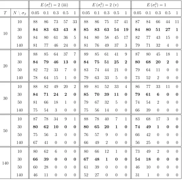
Table 2.1: The probability of 4ˆ being negative definite

E(σ2 i) = 2(iii) E(σ2i) = 2(v) E(σi2) = 1 T N \σβ 0.05 0.1 0.3 0.5 1 0.05 0.1 0.3 0.5 1 0.05 0.1 0.3 0.5 1 10 10 88 86 73 57 33 88 86 75 57 41 87 84 66 44 11 30 84 83 63 43 8 85 83 63 54 19 84 80 51 27 1 50 84 80 61 36 5 84 80 58 45 17 82 77 43 15 0 140 81 77 46 24 0 81 76 49 37 3 79 71 32 4 0 20 10 88 85 64 37 7 89 85 61 41 9 87 80 45 18 1 30 84 79 46 13 0 84 75 51 25 2 80 68 20 2 0 50 82 72 33 7 0 83 74 44 21 0 79 64 11 0 0 140 78 64 15 1 0 79 63 33 5 0 73 52 2 0 0 30 10 88 82 49 20 2 89 81 52 33 4 86 77 33 11 0 30 84 71 24 2 0 85 70 39 11 0 79 61 6 0 0 50 81 66 18 1 0 79 67 32 5 0 74 54 2 0 0 140 75 54 3 0 0 75 56 14 0 0 66 39 0 0 0 50 10 87 78 34 9 1 88 78 40 7 1 83 68 17 3 0 30 80 62 10 0 0 80 65 20 1 0 74 49 1 0 0 50 75 56 3 0 0 76 57 9 0 0 66 42 0 0 0 140 67 41 0 0 0 66 49 2 0 0 56 25 0 0 0 140 10 80 62 6 0 0 80 66 12 1 0 73 49 2 0 0 30 66 39 0 0 0 67 48 1 0 0 54 18 0 0 0 50 60 28 0 0 0 61 39 0 0 0 46 10 0 0 0 140 46 11 0 0 0 52 27 0 0 0 31 1 0 0 0

The probability (in percentage) of the estimator of4being negative definite (averaged across the7options) across the time dimension(T), the cross-section dimension(N), different degrees of coefficient heterogeneity (σβ), and the mean of the variance of the time-varying regression

disturbances(E(σ2

i)), for i = 1, .., N. The results shown in columns (iii) and (v) differ as in

the formerσ_i2∼unif[1,3]. In the latter,σ2_i ∼ϕ·unif[0.5,1.5] + (1−ϕ)·unif[4,6].

2. % can be quite high when σβ is small or moderate. If σβ = 0.05, the value

of % can be substantial even when T = 140 and N is also large. On the contrary, if σβ = 1, % is almost always equal to zero as soon as T is larger

(34)

3. The variance of the time-varying disturbances also plays an important role. Indeed, for a given degree of coefficient heterogeneity, as σ2

i increases, the

second term of (2.8) raises. Consequently, the probability that the estimator of the random coefficient covariance matrix is negative definite increases.

4. Whether %is large or small depends on the value of σβ relative to the σi’s,

the standard deviations of the time-varying regression disturbances. This means that even though σβ is high, % can be still far from zero if E(σi2) is

very large.

2.4.3 Regression Analysis

To corroborates the findings of the theoretical analysis and the insights emerged in the descriptive analysis, we run the following cross-section regression:

ym =α+zm0 θ+um, m = 1, .., M,

whereM = 4200. The depedent variableym measures the probability of4ˆ being

negative definite within each DGP, and it is computed as

ym =P r ˆ 4<0= PH h=1W ˆ 4(h) _<₀ H ,

where_Wis a binary indicator that takes the value1if4ˆ(h) _<₀_{(in a matrix sense)} and 0otherwise. The vector zm may include the following explanatory variables:

• the time dimension, T, and the number of units, N,

• the values of the intercept(c)and slope parameter (β)in (2.21),

• the degree of coefficient heterogeneity,σc =σβ,

• the average standard deviation of the regression disturbances,¯σ=N−1PN i=1σi, • a measure of the signal-to-noise ratio, σβ/¯σ,

(35)

• the bias of the Mean Group estimator of ψ = (c, β)0,

• the cross-section averages of the absolute value of the biases of the OLS estimators: 1 N N X i=1 1 H H X h=1 ˆ ψ_i(h) ! −ψ ,

• the trace of the root mean square errors (RMSE) of the Mean Group es-timator,

• the trace of the RMSE of the OLS estimators, averaged across units:

AvRM SEψˆi = 1 N N X i=1    v u u t 1 H H X h=1 ˆ ψ_i(h)−ψ_i(h) ψˆ_i(h)−ψ_i(h) 0    .

We estimate the model by OLS. Results are shown in Table 2.2. In par-enthesis, we report the t-tests computed using White (1980) heteroskedasticity-robust standard errors.7

Main Findings. In the simplest specification (1), we regress our dependent

variables on a constant, the time dimension (T), the number of units (N), the degree of coefficient heterogeneity (σβ), and the average of the time-varying

re-gression disturbances’ standard deviations (¯σ). We then include the value of c

and β used in equation (2.21) to simulate the data. As expected, the constant, which is approximatively equal to 70%, is statistically significant. One standard deviation increase of σβ statistically significantly reduces the probability of 4ˆ

being negative definite (%) of around70%. The conditional variability of the data is also a significant predictor: one standard deviation increase of σ¯ is associated with a statistically significant increase in the dependent variable of 5%.

7_{When calculating the robust standard errors, we make the adjustment for degrees of}

(36)

Table 2.2: The drivers of the random coefficient covariance’s negative definiteness problem P r4ˆ <0 (1) (2) (3) (4) (5) (6) constant 0.696 0.695 0.744 0.562 0.521 0.536 (82.77) (71.27) (77.33) (58.52) (46.54) 45.031 T -0.002 -0.002 -0.002 -0.001 -0.001 -0.001 (-32.04) (-32.03) (-28.99) (-12.85) (-9.38) -11.596 N -0.001 -0.001 -0.001 -0.001 -0.001 -0.001 (-21.52) (-21.52) (-19.09) (-23.73) (-8.41) -10.312 σβ -0.697 -0.697 -1.160 -0.802 -1.218 (-91.69) (-91.66) (-58.12) (-71.60) -45.356 ¯ σ 0.052 0.052 0.018 0.015 0.020 (21.59) (21.60) (7.31) (5.31) 7.318 σβ/σ¯ -0.639 (-49.98) c 0.003 0.002 0.004 (0.31) (0.18) 0.477 β 0.001 0.001 -0.002 (0.11) (0.152) -0.333 bias(ˆcmg) -0.198 -0.083 (-0.32) -0.132 biasβˆmg 0.239 0.347 (0.30) 0.449 Av(|bias(ˆci,ols)|) 13.099 12.346 (17.26) 12.215 Av bias ˆ βi,ols 14.246 13.366 (12.09) 11.058 RM SE ˆ ψM G 0.373 0.301 (14.78) 10.777 RM SE ˆ ψi,ols 0.163 -0.044 (16.90) -2.863 R2 _0.675 _0.675 _0.576 _0.728 _0.713 _0.734 Theil Adj. R2 _0.675 _0.675 _0.576 _0.728 _0.713 _0.733

We regress the probability of4ˆ being negative definite on a number of explanatory variables. The values of the OLS estimators and their corresponding t-ratios (in parentheses) are repor-ted. We use White (1980) heteroskedasticity-robust standard errors with the adjustment for degrees of freedom suggested by MacKinnon and White (1985). Bold values denotes statistical significance at5%level or lower.

(37)

At the same time, an one unit increase in T and N causes a 0.2% and 0.1%

decrease of %, respectively. On the contrary, the coefficients associated with the value of the constant and intercept parameters (c and β) are not statistically significant. These findings are consistent across all other specifications.

In a third regression (3), we replaceσβ andσ¯ with a measure of the

signal-to-noise ratio(σβ/σ¯).8 An one standard deviation increase of the latter statistically

significantly decreases the probability of 4ˆ being negative definite by 64%. The R-squared is smaller in the third specification, suggesting that including bothσβ

and σ¯ separately improves the goodness of fits.

Given that4ˆ, described in equation (2.8), is a plug-in estimator, we also test whether the finite sample performances (in terms of bias and RMSE) of both the Mean Group estimator of c and β, and the OLS estimators of the unit-specific regression coefficients affect the probability of 4ˆ being negative definite. The regression analyses (4) to (6) corroborate this hypothesis. For instance, a 1%

increase in the cross-section averages of the absolute value of the biases of the OLS estimates raises %of around 12to 14%.

2.4.4 Finite-Sample Consequences

As shown in Table 2.1, the unbiased estimator of the random coefficient covari-ance matrix defined in equation (2.8), is likely to be negative definite in many circumstances. This is often the case in many empirical applications. To overcome the problem, Swamy (1971) suggests replacing this estimator by 4ˆ1, defined in equation (2.9). The latter is nonnegative definite and is consistent whenT tends to infinity. However, as reported in Table 2.3 , it can be severely biased in small samples.

8_{We have also considered other measures of signal-to-noise ratio:} _N−1PN

i=1 σ2 β/σε2i , N−1PN i=1(σβ/σεi), and σ2 β/¯σ 2_{, where} _σ_¯2 ₌ _N−1PN i=1σ 2

εi. They yield very similar

res-ult. Therefore, we only report results obtained using(σβ/¯σ), with σ¯ = N−1P N

i=1σεi as the

corresponding regression coefficient has larger economic value and it is associated with a larger t-ratio. Both theR2_{and the Theil’s adjusted} _R2 _{are also relatively larger in the latter case.}

(38)

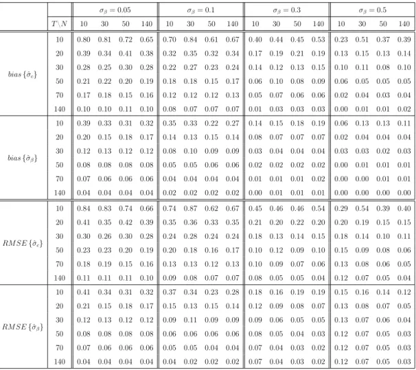
Table 2.3: Bias and root mean square errors of 4ˆ1

σβ= 0.05 σβ= 0.1 σβ= 0.3 σβ= 0.5 T\N 10 30 50 140 10 30 50 140 10 30 50 140 10 30 50 140 bias{ˆσc} 10 0.80 0.81 0.72 0.65 0.70 0.84 0.61 0.67 0.40 0.44 0.45 0.53 0.23 0.51 0.37 0.39 20 0.39 0.34 0.41 0.38 0.32 0.35 0.32 0.34 0.17 0.19 0.21 0.19 0.13 0.15 0.13 0.14 30 0.28 0.25 0.30 0.28 0.22 0.27 0.23 0.24 0.14 0.12 0.13 0.15 0.10 0.11 0.08 0.10 50 0.21 0.22 0.20 0.19 0.18 0.18 0.15 0.17 0.06 0.10 0.08 0.09 0.06 0.05 0.05 0.05 70 0.17 0.18 0.15 0.16 0.12 0.12 0.12 0.13 0.05 0.07 0.06 0.06 0.02 0.04 0.03 0.04 140 0.10 0.10 0.11 0.10 0.08 0.07 0.07 0.07 0.01 0.03 0.03 0.03 0.00 0.01 0.01 0.02 bias{σβˆ } 10 0.39 0.33 0.31 0.32 0.35 0.33 0.22 0.27 0.14 0.15 0.18 0.19 0.06 0.13 0.13 0.11 20 0.20 0.15 0.18 0.17 0.14 0.13 0.15 0.14 0.08 0.07 0.07 0.07 0.02 0.04 0.04 0.04 30 0.12 0.13 0.12 0.12 0.08 0.10 0.09 0.09 0.03 0.04 0.04 0.04 0.03 0.03 0.02 0.03 50 0.08 0.08 0.08 0.08 0.05 0.05 0.06 0.06 0.02 0.02 0.02 0.02 0.00 0.01 0.01 0.01 70 0.07 0.06 0.06 0.06 0.04 0.04 0.04 0.04 0.01 0.01 0.01 0.02 0.00 0.00 0.01 0.01 140 0.04 0.04 0.04 0.04 0.02 0.02 0.02 0.02 0.00 0.01 0.01 0.01 0.00 0.00 0.00 0.00 RM SE{σcˆ} 10 0.84 0.83 0.74 0.66 0.74 0.87 0.62 0.67 0.45 0.46 0.46 0.54 0.29 0.54 0.39 0.40 20 0.41 0.35 0.42 0.39 0.35 0.36 0.33 0.35 0.21 0.20 0.22 0.20 0.20 0.19 0.15 0.15 30 0.30 0.26 0.30 0.28 0.24 0.28 0.24 0.24 0.18 0.13 0.14 0.15 0.18 0.14 0.10 0.11 50 0.23 0.23 0.20 0.19 0.20 0.18 0.16 0.17 0.10 0.12 0.09 0.10 0.15 0.09 0.08 0.06 70 0.18 0.19 0.15 0.16 0.13 0.13 0.12 0.13 0.10 0.09 0.07 0.06 0.13 0.08 0.06 0.05 140 0.11 0.11 0.11 0.10 0.09 0.08 0.07 0.07 0.08 0.05 0.05 0.04 0.12 0.07 0.05 0.04 RM SE{ˆσβ} 10 0.41 0.34 0.31 0.32 0.37 0.34 0.23 0.28 0.18 0.16 0.19 0.19 0.15 0.16 0.14 0.12 20 0.21 0.15 0.18 0.17 0.15 0.13 0.15 0.14 0.12 0.09 0.08 0.07 0.13 0.08 0.07 0.05 30 0.12 0.13 0.12 0.12 0.09 0.11 0.09 0.09 0.09 0.06 0.05 0.05 0.13 0.07 0.06 0.04 50 0.08 0.08 0.08 0.08 0.06 0.06 0.06 0.06 0.08 0.05 0.04 0.03 0.12 0.07 0.05 0.03 70 0.07 0.06 0.06 0.06 0.05 0.05 0.04 0.04 0.07 0.04 0.03 0.02 0.12 0.07 0.05 0.03 140 0.04 0.04 0.04 0.04 0.04 0.02 0.02 0.02 0.07 0.04 0.03 0.02 0.12 0.07 0.05 0.03

The bias and root mean square errors (RMSE) of the square root of the diagonal elements of 4ˆ1, when E σi2

= 1 and (c, β) = (0,0.5) (Option 2), for various degree of coefficient heterogeneity (σβ=σc), across different time (T) and cross-section dimensions (N).

Therefore, it is important to assess the finite-sample consequences of using 4ˆ1 as an estimator of 4. The aim of this subsection is to provide some evidence on whether it is appropriate to rely on the asymptotic properties of this estimator as the basis for inference in finite samples. Without loss of generality, we focus on the results obtained from Option2, where (c, β) = (0,0.5). We only show results obtained when E(σ2

i) = 1, for various degrees of coefficient heterogeneity. The

(39)

increases.9 Further analyses are available in an online Appendix.

Notation. Hereafter, we use the following notation to avoid repetition. We let

ψ0 = (c, β) 0

= (0,0.5)0 be the true vector of average effects. The true random coefficient covariance matrix, 4, is diagonal, where σ2

c and σ2β are the (1,1)and (2,2)entries, respectively. We let

ˆ ψGLS = N X i=1 X_i0V_i−1Xi !−1 _N X i=1 X_i0V_i−1yi ! , (2.22) and Φ =varψˆGLS = N X i=1 X_i0V_i−1Xi !−1 , (2.23)

whereVi =Xi4Xi0+σ2iIT, be the infeasible GLS estimator ofψ, and the infeasible

covariance matrix ofψˆGLS, respectively. The feasible GLS estimator,ψˆF GLS, and

an estimator of Φ, denotedΦˆ, are obtained by replacing σ2

i and4byσˆi2 and 4ˆ1, as defined in (2.7) and (2.9), respectively.

Accuracy of Estimated Standard Errors

To examine the consequences of overestimating the true random coefficient vari-ances when testing hypotheses, we consider the ratio of the estimated standard errors (of the average effects) to the infeasible standard errors, obtained by tak-ing the square root of the diagonal elements of Φˆ and Φ respectively. Another measure of interest for inference is the accuracy of the estimated standard errors as approximations to the correct sampling standard deviation of the estimator of ψ.10 _{These ratios should ideally be equal to one. Results reported in Table}

9_{Case (}_v_{) is particularly interesting. Even though the variance of most of the units varies}

between 0.5 and 1.5, as in case (ii), the presence of some outliers, such that E σ_i2 = 2, considerably worsen the accuracy of inference.

10_The _accuracy _of _the _estimated _standard _errors _is _computed _as _the _ratio _of

B−1PB

b=1 q

( ˆΦb)kk

to the sampling standard deviation of ψˆk, given by the square root

of(B−1)−1PB b=1 ˆ ψk,(b)− ¯ ˆ ψk 2 , whereψ¯ˆk=B−1P B b=1ψˆk,(b), fork= 1,2.

(40)

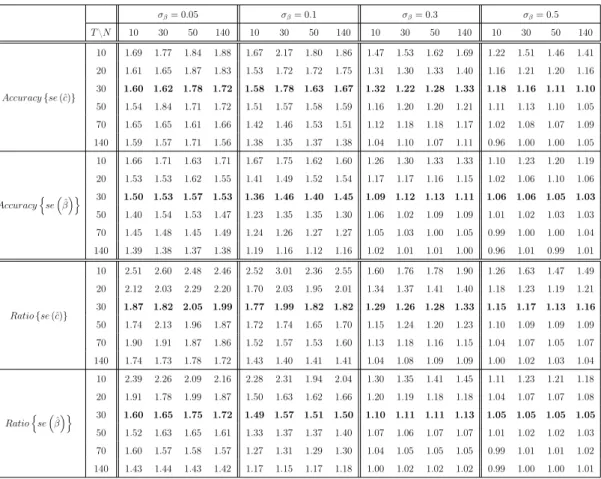
2.4, show that relying exclusively on the asymptotic properties of 4ˆ1 may lead to invalid inference in finite samples. The estimated standard errors are upwards biased for the vast majority of cases. These biases can be substantial unless T

and N or the degree of coefficient heterogeneity (σβ) are large. However, if the

coefficient dispersion is low, the estimated standard errors can be largely over-estimated even when both T and N are equal to 140. These biases can in turn significantly affect inference.

Table 2.4: Accuracy of estimated standard errors

σβ= 0.05 σβ= 0.1 σβ= 0.3 σβ= 0.5 T\N 10 30 50 140 10 30 50 140 10 30 50 140 10 30 50 140 Accuracy{se(ˆc)} 10 1.69 1.77 1.84 1.88 1.67 2.17 1.80 1.86 1.47 1.53 1.62 1.69 1.22 1.51 1.46 1.41 20 1.61 1.65 1.87 1.83 1.53 1.72 1.72 1.75 1.31 1.30 1.33 1.40 1.16 1.21 1.20 1.16 30 1.60 1.62 1.78 1.72 1.58 1.78 1.63 1.67 1.32 1.22 1.28 1.33 1.18 1.16 1.11 1.10 50 1.54 1.84 1.71 1.72 1.51 1.57 1.58 1.59 1.16 1.20 1.20 1.21 1.11 1.13 1.10 1.05 70 1.65 1.65 1.61 1.66 1.42 1.46 1.53 1.51 1.12 1.18 1.18 1.17 1.02 1.08 1.07 1.09 140 1.59 1.57 1.71 1.56 1.38 1.35 1.37 1.38 1.04 1.10 1.07 1.11 0.96 1.00 1.00 1.05 Accuracy n se ˆ β o 10 1.66 1.71 1.63 1.71 1.67 1.75 1.62 1.60 1.26 1.30 1.33 1.33 1.10 1.23 1.20 1.19 20 1.53 1.53 1.62 1.55 1.41 1.49 1.52 1.54 1.17 1.17 1.16 1.15 1.02 1.06 1.10 1.06 30 1.50 1.53 1.57 1.53 1.36 1.46 1.40 1.45 1.09 1.12 1.13 1.11 1.06 1.06 1.05 1.03 50 1.40 1.54 1.53 1.47 1.23 1.35 1.35 1.30 1.06 1.02 1.09 1.09 1.01 1.02 1.03 1.03 70 1.45 1.48 1.45 1.49 1.24 1.26 1.27 1.27 1.05 1.03 1.00 1.05 0.99 1.00 1.00 1.04 140 1.39 1.38 1.37 1.38 1.19 1.16 1.12 1.16 1.02 1.01 1.01 1.00 0.96 1.01 0.99 1.01 Ratio{se(ˆc)} 10 2.51 2.60 2.48 2.46 2.52 3.01 2.36 2.55 1.60 1.76 1.78 1.90 1.26 1.63 1.47 1.49 20 2.12 2.03 2.29 2.20 1.70 2.03 1.95 2.01 1.34 1.37 1.41 1.40 1.18 1.23 1.19 1.21 30 1.87 1.82 2.05 1.99 1.77 1.99 1.82 1.82 1.29 1.26 1.28 1.33 1.15 1.17 1.13 1.16 50 1.74 2.13 1.96 1.87 1.72 1.74 1.65 1.70 1.15 1.24 1.20 1.23 1.10 1.09 1.09 1.09 70 1.90 1.91 1.87 1.86 1.52 1.57 1.53 1.60 1.13 1.18 1.16 1.15 1.04 1.07 1.05 1.07 140 1.74 1.73 1.78 1.72 1.43 1.40 1.41 1.41 1.04 1.08 1.09 1.09 1.00 1.02 1.03 1.04 Ratio n se ˆ β o 10 2.39 2.26 2.09 2.16 2.28 2.31 1.94 2.04 1.30 1.35 1.41 1.45 1.11 1.23 1.21 1.18 20 1.91 1.78 1.99 1.87 1.50 1.63 1.62 1.66 1.20 1.19 1.18 1.18 1.04 1.07 1.07 1.08 30 1.60 1.65 1.75 1.72 1.49 1.57 1.51 1.50 1.10 1.11 1.11 1.13 1.05 1.05 1.05 1.05 50 1.52 1.63 1.65 1.61 1.33 1.37 1.37 1.40 1.07 1.06 1.07 1.07 1.01 1.02 1.02 1.03 70 1.60 1.57 1.58 1.57 1.27 1.31 1.29 1.30 1.04 1.05 1.05 1.05 0.99 1.01 1.01 1.02 140 1.43 1.44 1.43 1.42 1.17 1.15 1.17 1.18 1.00 1.02 1.02 1.02 0.99 1.00 1.00 1.01

Accuracy{se(·)}denotes the ratio of the estimated standard errors (of the average effects) to the sampling standard deviations. Ratio{se(·)} denotes the ratio of the estimated standard errors to the infeasible standard errors. Results obtained using Option2, whenE(σ_i2) = 1.

(41)

Hypothesis tests

To test the hypothesisψ =ψ, forψa knownK×1vector, Swamy (1970) suggests the following criterion:

F ψ, ψ,ˆ Φˆ= N −K K(N −1) ˆ ψ−ψ 0 ˆ Φ−1ψˆ−ψ. (2.24)

The asymptotic distribution of the test is F, withK, N−K degrees of freedom.

Empirical Moments of the F-statistic. We now study the finite-sample

properties of the distribution of (3.50). In particular, we examine the empir-ical distributions of Fψˆk,GLS, ψ0,k,Φkk

, and F ψˆk,F GLS, ψ0,k,Φˆkk

, computed under the null hypothesis that the estimator (of interest) of ψk is equal to the

corresponding true value used to generate the data, ψ0,k, for k = 1,2.11 We

then compare the mean, standard deviation, skewness, and excess kurtosis of these two empirical distributions with the corresponding population moments of a F-distribution with 1, N −1 degrees of freedom. Results are reported in Table 2.5. In many cases, the means and standard deviations of the distributions of the F-statistics based on the infeasible GLS estimator are relatively close to the true means and standard deviations. This is not the case when considering the distributions of the F-statistics based on the feasible GLS estimator. The means and standard deviations of the latter can be substantially smaller than the values associated with a F-distribution with1,N−1degrees of freedom. Results worsen when testing hypothesis about the intercept rather than slope parameters. These results are in line with the fact that 4ˆ1 is often upwards biased. The skewness and excess-kurtosis of the distribution of the F-statistics based on both feasible and infeasible GLS estimators, can be far from the corresponding population moments unless N is large.

11_Φ

(42)

Table 2.5: Empirical moments of F-statistics

β Mean Standard Deviation Skewness Excess-Kurtosis

T\N 10 30 50 140 10 30 50 140 10 30 50 140 10 30 50 140 F1,N−1 1.29 1.07 1.04 1.01 2.30 1.61 1.52 1.45 6.71 3.37 3.12 2.92 214.50 19.23 15.61 13.11 Infeasible 10 0.96 1.06 0.97 1.04 1.37 1.47 1.47 1.47 2.86 2.40 3.17 2.60 11.67 7.23 14.87 8.78 20 1.01 1.00 0.94 0.99 1.47 1.56 1.35 1.41 2.92 3.65 2.86 2.95 12.66 21.85 11.26 12.12 30 1.02 0.98 1.03 0.97 1.38 1.42 1.40 1.41 2.44 2.65 2.35 2.92 7.69 9.43 7.06 12.41 50 1.08 0.96 0.96 1.06 1.58 1.33 1.33 1.53 3.06 2.65 2.52 2.73 13.51 9.55 8.06 9.99 70 1.00 1.02 0.98 0.98 1.42 1.47 1.46 1.49 3.74 3.41 3.32 3.12 28.41 19.85 17.49 14.11 140 0.96 0.96 1.07 1.02 1.31 1.33 1.43 1.44 2.64 2.61 2.58 2.51 9.77 8.82 9.14 7.56 Feasible 10 0.37 0.34 0.39 0.39 0.56 0.48 0.55 0.54 3.48 2.95 2.77 2.61 18.91 13.18 11.11 10.25 20 0.55 0.46 0.44 0.43 0.86 0.72 0.63 0.64 3.86 3.42 2.90 3.24 23.48 17.91 12.25 15.69 30 0.58 0.48 0.51 0.48 0.85 0.70 0.69 0.69 3.25 3.59 2.49 2.97 15.13 26.34 8.97 12.46 50 0.71 0.56 0.56 0.59 1.14 0.81 0.79 0.85 3.59 3.04 2.74 2.83 18.00 13.08 10.30 11.52 70 0.70 0.64 0.62 0.62 1.09 0.97 0.94 0.96 4.45 4.48 3.34 3.31 37.08 40.21 17.46 16.76 140 0.79 0.76 0.82 0.75 1.27 1.11 1.14 1.06 4.36 3.06 2.74 2.56 34.97 13.97 10.30 8.02

c Mean Standard Deviation Skewness Excess-Kurtosis

T\N 10 30 50 140 10 30 50 140 10 30 50 140 10 30 50 140 F1,N−1 1.29 1.07 1.04 1.01 2.30 1.61 1.52 1.45 6.71 3.37 3.12 2.92 214.50 19.23 15.61 13.11 Infeasible 10 1.09 1.01 0.96 1.01 1.43 1.37 1.40 1.43 2.34 2.50 2.74 2.67 7.00 8.57 9.76 9.27 20 0.99 1.00 1.02 0.97 1.40 1.43 1.41 1.44 2.87 2.94 2.72 4.32 12.95 11.53 10.39 38.22 30 1.02 0.95 0.99 1.01 1.45 1.37 1.40 1.38 2.56 3.05 2.73 2.73 8.44 15.32 10.26 11.25 50 1.02 1.00 0.98 0.98 1.54 1.36 1.37 1.40 2.87 2.64 2.53 3.03 10.30 11.47 8.26 14.45 70 0.99 1.05 0.95 1.00 1.49 1.50 1.38 1.43 3.17 2.52 3.11 3.07 15.04 7.93 14.63 15.15 140 0.99 1.01 1.00 0.99 1.35 1.50 1.43 1.34 2.43 2.93 2.78 2.33 7.81 11.53 10.54 6.71 Feasible 10 0.38 0.22 0.31 0.29 0.59 0.30 0.43 0.43 4.76 2.47 2.55 2.77 45.68 8.11 8.78 10.07 20 0.46 0.35 0.34 0.33 0.77 0.53 0.49 0.47 5.41 3.53 2.79 3.14 51.13 19.04 10.70 14.86 30 0.43 0.32 0.38 0.36 0.62 0.44 0.55 0.49 2.69 2.93 2.76 2.67 9.45 13.93 11.42 10.02 50 0.47 0.42 0.40 0.40 0.70 0.60 0.57 0.58 3.11 3.05 2.80 3.19 13.65 13.79 11.90 14.99 70 0.53 0.49 0.44 0.44 0.81 0.71 0.65 0.62 3.72 2.95 3.05 2.90 22.65 12.36 13.24 13.28 140 0.57 0.57 0.54 0.53 0.86 0.92 0.78 0.73 3.27 4.21 2.85 2.52 16.53 31.53 11.26 8.51

Empirical moments of F-statistics across different sample sizes(T.N), when the data are gener-ated from Option2, withE(σ_i2) = 1, andσβ=σc = 0.1. In the upper panel, the test statistics

are constructed under the null hypothesisH0: β = 0.5 against the alternativeH1: β 6= 0.5. In the lower panel, the null hypothesis is H0: c = 0 againstH1: c 6= 0. Row “F1,N−1” reports the population moments of a F-distribution with 1, N−1 degrees of freedom. The empirical moments reported in “Infeasible” correspond to the F-statistics computed using the infeasible GLS estimator of ψ and the infeasible covariance matrix, Φ. “Feasible” is used to denote the empirical moments of the F-statistics, replacing the unknown components inψandΦby their estimators.

Power Performances. In Table 2.6 we report the empirical sizes of the

(43)

the alternative H1: ψk 6=ψ0,k. They are computed as the relative rejection

fre-quencies based on the critical regions of nominal size0.05of a F-distribution with

1, N −1 degrees of freedom. This allows us to evaluate the direct consequences of the various results described above for hypothesis tests.

Table 2.6: Empirical sizes based on F-statistics

σβ= 0.05 σβ= 0.1 σβ= 0.3 σβ= 0.5 T\N 10 30 50 140 10 30 50 140 10 30 50 140 10 30 50 140 sizeβGLSˆ 10 2.47 4.80 4.47 4.00 2.13 5.07 4.60 5.33 2.13 4.00 4.60 5.67 2.27 3.80 4.00 4.13 20 2.67 4.53 4.40 5.67 2.93 4.40 3.73 3.73 2.80 4.40 4.00 5.27 2.47 3.27 3.47 4.80 30 2.20 4.73 4.60 4.60 2.33 4.33 5.13 4.67 1.60 4.47 3.13 4.87 2.00 3.87 4.47 5.33 50 2.27 3.87 3.80 5.40 3.07 3.53 4.00 5.47 2.60 5.00 3.40 4.53 2.20 4.07 4.00 5.07 70 2.33 3.33 3.93 4.27 1.87 3.53 4.13 5.07 2.60 4.33 5.27 4.07 2.33 3.67 5.27 3.80 140 2.53 3.33 4.13 4.53 2.13 3.47 4.80 5.80 1.93 3.60 4.40 4.93 3.33 4.27 4.87 4.73 sizeβF GLSˆ 10 0.00 0.07 0.07 0.20 0.13 0.07 0.13 0.07 1.07 0.60 0.73 0.60 2.20 1.00 1.67 2.00 20 0.07 0.20 0.00 0.13 0.40 0.47 0.27 0.33 1.80 2.47 2.13 2.27 3.47 2.93 2.93 3.60 30 0.20 0.27 0.13 0.13 0.67 0.20 0.27 0.53 2.20 3.20 2.13 3.00 2.73 3.47 3.60 4.40 50 0.33 0.07 0.20 0.60 1.20 0.93 0.93 1.07 3.07 4.53 3.07 3.00 3.87 4.47 3.93 4.53 70 0.20 0.27 0.53 0.33 0.87 0.87 1.27 1.40 2.93 4.00 4.87 3.40 4.60 4.67 4.47 3.73 140 0.40 0.47 0.47 0.53 1.33 2.13 2.40 2.47 4.33 4.00 4.60 4.87 5.33 5.60 5.33 4.33 size(ˆcGLS) 10 2.33 4.00 4.33 4.27 2.53 3.93 3.80 4.53 1.93 3.87 3.47 4.40 2.33 3.47 3.67 5.33 20 2.47 4.53 3.93 4.27 2.13 3.87 3.93 4.07 3.20 4.33 5.27 4.27 3.00 3.60 4.00 5.53 30 2.60 5.00 3.80 5.13 2.73 3.60 4.13 5.13 1.67 4.27 4.07 3.93 2.27 3.87 4.33 6.60 50 2.60 4.00 4.53 4.13 3.13 3.80 4.40 4.80 2.13 4.80 3.93 5.33 2.33 3.07 3.53 5.13 70 2.00 4.40 5.27 4.53 2.53 4.80 3.80 4.60 3.00 4.20 3.00 3.73 2.27 3.20 4.87 4.07 140 2.07 4.80 3.47 4.00 2.07 4.27 4.13 4.67 1.93 4.13 4.73 4.47 2.87 5.33 5.00 4.73 size(ˆcF GLS) 10 0.07 0.07 0.00 0.00 0.07 0.00 0.00 0.00 0.20 0.27 0.47 0.20 1.20 0.40 0.53 0.53 20 0.13 0.07 0.13 0.07 0.40 0.20 0.07 0.07 0.73 0.53 1.27 0.67 1.73 1.47 1.80 2.07 30 0.07 0.13 0.13 0.07 0.07 0.07 0.07 0.13 0.73 1.40 1.20 0.60 1.80 2.33 2.60 3.53 50 0.07 0.07 0.13 0.00 0.20 0.27 0.20 0.27 1.67 1.73 1.80 1.80 2.13 2.27 2.60 3.00 70 0.00 0.07 0.13 0.13 0.33 0.47 0.33 0.27 2.60 1.87 1.93 1.93 3.53 2.40 3.80 3.00 140 0.27 0.13 0.27 0.20 0.33 1.20 0.73 0.47 3.00 3.47 3.00 3.60 5.27 5.47 5.00 3.87

Rejection frequencies (%) at5%nominal level obtained computing the F-statistic described in (3.50), under the null hypothesis H0: ψk =ψ0,k against the alternative H1: ψk 6=ψ0,k. βˆGLS

andcˆGLS denote the infeasible GLS estimator ofβ and crespectively. Similarly, the subscript

“FGLS ” stands for feasible GLS. The data are generated from Option2, withE(σ_i2) = 1.

The tests based on the feasible GLS estimation severely suffer from size distor-tions. Unless the degree of coefficient heterogeneity is quite high (e.g. σβ = 0.5),

(44)

close to zero due to the fact that the estimated standard errors are largely biased upward. Once again, the distortions are even more severe when testing about the intercept parameters.

To support these findings, we plot the power functions for the slope and intercept parameters in Figure 2.1 and 2.2 respectively. To save space, we only report results for the case with E(σ2

i) = 1 and σβ = 0.1.12

Figure 2.1: Rejection frequency (%) at the 5% nominal level, for the slope parameter (β), in the y-axis. They are computed using the F-statistic described in (3.50), under the null hypothesisH0: β=β against the alternativeβ 6=β. Different values ofβ are reported in the x-axis. The true value of β is0.5. The black lines and the red dotted lines denote the power performances of feasible and infeasible GLS estimators, respectively. Results obtained using Option2, withE(σ2_i) = 1andσβ= 0.1.

(45)

2.5. Conclusions 45

Figure 2.2: Rejection frequency (%) at the 5% nominal level, for the intercept parameter (c), in the y-axis. They are computed using the F-statistic described in (3.50), under the null hypothesis H0: c = c against the alternative c 6=c. Different values ofc are reported in the x-axis. The true value of c is 0. The black lines and the red dotted lines denote the power performances of feasible and infeasible GLS estimators, respectively. Results obtained using Option2, withE(σ2_i) = 1andσc= 0.1.

2.5 Conclusions

As in the error component model, the estimator of the coefficients’ covariance matrix in a random coefficient model is often negative definite. The aim of this study is to investigate the causes and effects of the problem. By running some Monte Carlo experiments, we show that the degree of coefficient heterogeneity relative to the (conditional) variability of the dependent variables plays a cru-cial role. The larger the coefficient dispersion and the precision of the regression disturbances (the inverse of the average variance of the time-varying errors), the lower the probability to observe a negative definite estimator of the random coef-ficient covariance matrix. An increase in the former has a larger effect than an increase in the latter. Similarly, this probability decreases as the time dimension

(46)

2.5. Conclusions 46

and the number of units get large, partly due to the fact that the performances (in terms of bias and RMSE) of individual OLS estimates and the Mean Group improves in large samples. It is known that when the time dimension goes to infinity, the negative definiteness problem vanishes.

We then demonstrate that relying on the asymptotic properties of the biased but consistent estimator of the random coefficient covariance matrix may lead to poor inference. Unless the time and cross-section dimensions, and/or the degree of coefficient dispersion are high, the estimated standard errors are largely upwards biased. The resulting hypothesis tests may suffer from considerable size distortions. The empirical sizes of the tests are substantially lower than the nominal levels. Results may worsen when the precision of the regression disturbances decreases. An estimation procedure which yields an unbiased and more efficient estimator of the random coefficient covariance and which performs relatively well in terms of accuracy of inference is proposed in Chapter 3.

(47)

2.6. Appendix 47

2.6 Appendix

2.6.1 Estimation of Parameters in the Presence of Serially

Correlated Disturbances

Swamy (1971) considers the estimation problem ofΩi when the the disturbances

follow an AR(1) process:

uit =φiui,t−1+it, 0<|φi |<1, (2.25)

and E(it) = 0, E(itjs) = σi2 if t = s and i = j, and 0 otherwise. For i = j,

E uiu0j =σ2 iΩi, where Ωi = 1 1−φ2 i            1 φi φ2i · · · φ T−1 i φi 1 φi · · · φTi−2 φ2 i φ 1 φ T−3 i .. . ... ... . .. ... φT_i −1 φT_i−2 φT_i −3 · · · 1            , and E uiu0j

= 0, if i6=j. A consistent estimator ofφi is given by

ˆ φi = PT t=2uˆituˆi,t−1 PT t=2uˆ2i,t−1 , (2.26)

where uît is the t-th element of uî, the vector of OLS residuals. An estimator of Ωi can be obtained by replacing φi byφî in Ωi. Note also that the inverse of Ωî