TIME SERIES MODELS
by D. F. Nicholls
A thesis submitted for the degree of
The results presented in this thesis are my own except where otherwise stated.
I was introduced to the subject of this thesis by my supervisor, Professor E.J.Hannan, who suggested many of the problems considered here and who guided me throughout their investigation. I am greatly indebted to him.
COKITE NTS
A c k n o w le d g e m e n ts i i i
Summary v i
CHAPTER 1 INTRODUCTION
1 . 1 P r e l i m i n a r y 1
1 .2 L i n e a r M odels 8
1 .3 E s t i m a t i o n o f t h e P a r a m e te r s o f F i n i t e L i n e a r M o d els 15
CHAPTER 2 A GOODNESS OF F IT TEST FOR VECTOR AUTOREGRESSIVE MODELS
2 . 1 I n t r o d u c t i o n 21
2 . 2 D e r i v a t i o n o f t h e T e s t 24
2 . 3 The C o m p u ta tio n a l P r o c e d u r e 32 2 . 4 A C o m p a riso n o f G o o d n ess o f F i t T e s t s 35
2 . 5 C o n c lu s io n 40
CHAPTER 3 THE ESTIMATION OF MOVING AVERAGE MODELS
3 . 1 I n t r o d u c t i o n 42
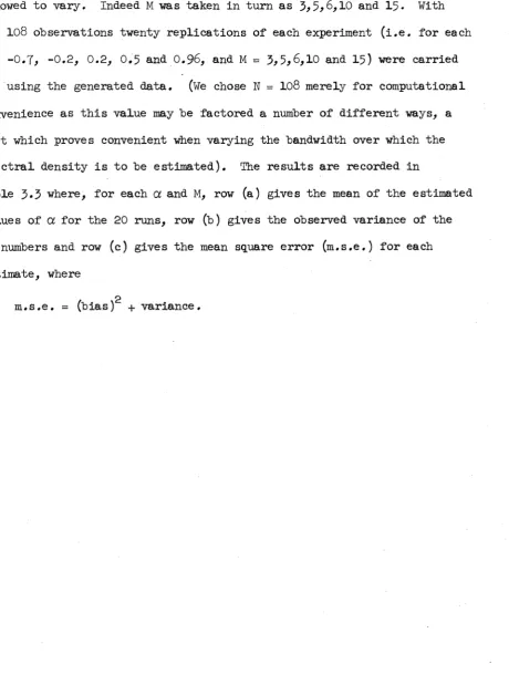
3
„2 C o n v e rg e n c e o f t h e I t e r a t i v e P r o c e d u r e 47 3 . 3 An E x t e n s i o n o f t h e E s t i m a t i o n P r o c e d u r e 523.4
A l t e r n a t i v e E s t i m a t i o n P r o c e d u r e s 573 .5 C o n c lu s io n 64
CHAPTER 4 THE ESTIMATION OF MIXED AUTOREGRESSIVE MOVING AVERAGE MODELS WITH EXOGENOUS VARIABLES
4.1 Introduction
67
4.2 The Estimation Procedure 72
4.3 The Distribution of the Estimates 8l
4.4 The Computational Procedure 102
4.5 Numerical Results 108
4.6 Conclusion 112
CHAPTER 3 DISTRIBUTED LAG MODELS
5.1 Introduction 11^
5.2 A Test for the Equality of the Parameters ll6
5.3
Estimation and Properties of the Coefficients 1185.4
Summary 123CHAPTER 6 EXTENSIONS TO THE VECTOR MODEL
6.1 The Vector Model 126
6.2 The Estimation Procedure and the Distribution
of the Estimates 128
6.3 The Computational Procedure 139
6.4 Conclusion 1 ^
This thesis presents an investigation of a number of inference problems associated with linear time series models. Two linear models which are of fundamental importance in the analysis of time series are the moving average model and the autoregressive model. It is models such as these, and models
constructed from them, with which we shall be concerned. The chapters may be summarized as follows: after a brief outline of the basic concepts of
spectral theory chapter 1 is concerned with a discussion of the properties of a number of linear time series models. This introductory chapter
concludes with a description of the estimation procedure, based on spectral methods, which is applied in the latter part of this thesis to obtain
efficient estimates of the coefficients of mixed regression, autoregression, moving average and distributed lag models.
In chapter 2 a goodness of fit test is derived for the vector
autoregressive model and an outline given of the computational procedure to be followed when applying the test. This test is compared with various other goodness of fit tests (for autoregressive models) occurring in the literature, the advantages and disadvantages of each being discussed.
Chapter 3 commences with a description of a procedure (due to Hannan [2 5]) for the efficient estimation of the coefficients of moving average models. After examining the rate of convergence of the iterative procedure
(in the case of the first order moving average model) associated with this method, an extension of Hannan’s procedure is described. This extension is introduced so as to prevent the estimation procedure from, on some
Finally in this chapter Hannan’s estimation procedure is compared with two other methods due to Durbin [14].
Chapter 4 is concerned with the derivation of a method for the
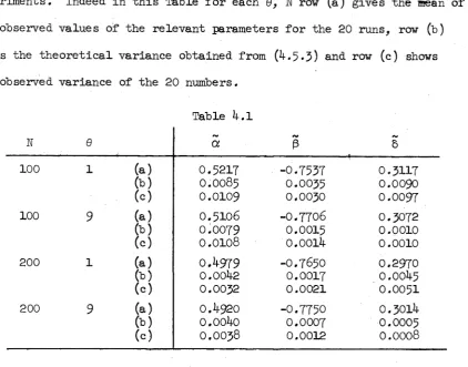
estimation of the coefficients of mixed autoregressive moving average models with exogenous variables. This procedure, which is based on the method of maximum likelihood, gives estimates which are shown to be asymptotically normally distributed and (asymptotically) efficient. After outlining the computational procedure for the application of this method, the results of a number of numerical experiments, using generated data, are presented in
section 4.5. As we see from that section, these results help to illustrate the theoretical results obtained.
1.1 Preliminary
We shall in this section introduce the basic definitions and
terminology which will be used throughout this thesis. In general no
attempt will be made to present rigorous derivations of the theory to be outlined since the current literature contains an increasing number of excellent introductions to the spectral theory of time series (e.g. Whittle [55]> Grenander and Rosenblatt [18], Hannan [22], [26], Jenkins and Watts [31]* Parzen [44] and Anderson [3] to name a few). For the purpose of this thesis Hannan [26] has been taken as the basic reference and we shall, in what follows, make reference to many of the results derived in that book.
Let us consider a time series (x(n); n = 0,+l,..,}, where x(n) is a vector of p components taken at time n, i.e. x / (n) = (x,(n)...x (n)).
P
We shall (unless otherwise stated) assume that the mean is zero so that for j
=
1,
...,p; n=
0,+l,...,
E(xj(n)) = 0 .
Furthermore we define the covariance matrix of this process to be r(m,n), where
E(x(m)x/ (n)) = r(m,n).
The series [x(n)j n = 0,+l, is said to be second order (or wide sense)
stationary if
E(x(m)x/ (n)) = r(0,n-m) = p(n-m) say, (l.l.l)
i«e. the covariance matrix depends only on the distance (n-m) between the
two observations being considered.1 If 7 (n) is the element in row j
Jk
column k (j,k = 1, ...,p) of
r(n)
then 7.An)
= 7 . (-n
), i.e.r(n) = r'(-n)
(where r/ (n) is the transpose of the matrix r(n)). It is often convenient
to work in terms of the serial correlations p (n) (which are scale free),
Jk where
i p jk(n) = b k (n)/(7jj(o)7k k
(o))2-For j = k we call these the autocorrelations and use the notation
Pk (n) = 7k (n)/rk (o)
If
r(n)
is the covariance matrix of a stationary vector process, then by Bochner's theoremr(n) =
f
elnAdF(A),
(1.1.2)
d -7T
where F(A) is a matrix with Hermitian non-negative increments i.e.
F(A^)-F(A2 ) 0, A^ ^ A2 ‘ This function F(a) is uniquely defined if
we require that (i) lim F(A) = 0, (ii) F(a) is continuous from the right.
A*-00
It is called the spectral distribution matrix and since it is Hermitian
f (A) = F / (-A). Rewriting dF(A) in the form
dF(A) = \ (dC(A)-idQ(A)) A > 0,
= dC (A) A = 0,
( i d . 2) becomes
r (n) (co s nA d C (A )+ sin nA dQ (A ))
C(A) an d Q(A) a r e r e f e r r e d t o a s th e c o s p e c t r a l an d q u a d r a t u r e s p e c t r a l d i s t r i b u t i o n m a tr ic e s r e s p e c t i v e l y .
Suppose F(A ) i s assum ed t o b e a b s o l u t e l y c o n tin u o u s . Then ( 1 .1 . 2 ) may be e x p r e s s e d i n th e form
r ( n ) = T e inAf(A )dA
- I T
(c (A )c o s n A + q(A )sin nA)dA, ( 1 * 1 .3 ) ^ o
w here now f ( A ) , c (A ), q(A ) a r e r e s p e c t i v e l y th e s p e c t r a l d e n s i t y , th e
c o s p e c t r a l d e n s i t y an d th e q u a d r a t u r e s p e c t r a l d e n s i t y m a t r i c e s . F u rth e rm o re from ( 1 . 1 . 3 ) i t f o llo w s t h a t
f (A) = (27r ) " 1 Z r ( n ) e " ln A . ( 1 . 1 . 4 )
n = - c o
J u s t a s ( 1 . 1 . 2 ) r e p r e s e n t s a t r a n s f o r m a t i o n o f t h e c o v a r ia n c e m a tr ix from t h e tim e t o th e f r e q u e n c y dom ain, t h e r e e x i s t s a s i m i l a r
t r a n s f o r m a t i o n (o r s p e c t r a l r e p r e s e n t a t i o n ) f o r x ( n ) . In d e e d we may l e t
(n) -in Adz (A)
-TV
(co s nA d |( A ) + s i n nA d 'n (A )), ( 1 . 1 . 5 )
w here z(A ) i s a com plex v e c t o r p r o c e s s o f o r th o g o n a l in c re m e n ts w ith dz(A ) = i( d |( A ) + i d i i ( A ) ) A > 0,
dz*((j.) r e p r e s e n t s t h e t r a n s p o s e d c o n j u g a t e o f d z ( q ) , w h ile 6 i s t h e
A^M-u s A^M-u a l K r o n e c k e r f A^M-u n c t i o n i . e . 6^
A,p
i s u n i t y when A = u an d z e r o o t h e r w i s e . F u r th e r m o r e t h e o n l y non z e r o c o v a r i a n c e s o f d | ( A ) , dr)(A) a r eE ( d | ( A ) d £ '( p ) ) = E (dri(A )dT i/(|i)) = 5 a c ( A ) ,
E ( d £ ( A ) d t ) '( n ) ) = - E ( d i i ( A ) d | / ( | i ) ) = S, dQ(A).
I n p r a c t i c e C(A) an d q(a) a r e r e p l a c e d "by two o t h e r e x p r e s s i o n s ,
w h ich we s h a l l d i s c u s s o n l y f o r t h e a b s o l u t e l y c o n t i n u o u s c a s e ( i . e . t h a t where dF'(A) = f(A )d A , so t h a t dC(A) = c(A)dA an d dQ(A) = q (A )d A ). We i n t r o d u c e t h e q u a n t i t i e s
4
(A)4 ;
a
>+4(
a
)
c j j (A,ck k (A)
if m^r
VA
T
f
a ™
’
9 j k (A) = t a n _ 1 ( q j k ( A ) / c J k ( A )),
where c (A), q . , (A) an d f (A) a r e t h e e l e m e n t s i n row j column k
J k JK JK
( j , k = 1, . . . , p ) o f c ( A ) , q(A) an d f ( A ) r e s p e c t i v e l y , a . , (A) an d 0 (a)
JK JK
a r e c a l l e d t h e c o h e r e n c e a n d t h e p h a s e r e s p e c t i v e l y an d a r e two
c h a r a c t e r i s t i c s m e a s u r i n g t h e d ep en d en ce o f x . ( n ) on x ( n ) . ( in d e e d t h e
J K
c o h e r e n c e m e a s u r e s t h e s t r e n g t h o f a s s o c i a t i o n i n t h e s e n s e o f maximum c o r r e l a t i o n o b t a i n e d b y r e p h a s i n g xk (n ) r e l a t i v e t o x^.(n) "by
N-n
C (n) = (N -n) E x (m )x / (m+n) n ^ 0, ( 1 .1 . 6 ) m=l
C (-n ) = C7 ( n ) .
(The e le m e n ts o f C (n) a r e , a t ti m e s , r e f e r r e d t o a s th e sam ple s e r i a l
c o v a r ia n c e s w h ile th e d ia g o n a l e le m e n ts ,- a r e c a l l e d t h e sam ple a u t o c o v a r i a n c e s ) . C (n) i s som etim es d e f in e d w ith t h e d i v i s o r (N -n) r e p la c e d b y N. A lth o u g h
t h e d i v i s i o n b y N makes C (n) a b i a s e d e s t i m a t o r , a s P a rz e n [45] p o i n t s o u t t h i s a l t e r n a t i v e e s t i m a t e o f r ( n ) h a s two d e s i r a b l e p r o p e r t i e s . F i r s t l y
i t l e a d s t o a s m a l le r mean s q u a re e r r o r f o r a g iv e n sam ple th a n d o es th e u n b ia s e d one an d s e c o n d ly t h e b i a s e d e s t i m a t o r i s p o s i t i v e d e f i n i t e , w h e re a s th e u n b ia s e d e s t i m a t o r i s n o t . (F o r some m a tr ix C (n ), i f a / C (n )a = c (n ) ( s a y ) f o r a l l a ^ 0, th e n C (n) i s p o s i t i v e d e f i n i t e i f
£L
N ^
E E c (£ -m )z (£ )z (m ) > 0 , £ ,m = l a
f o r some z ( £ ) n o t a l l z e r o . I f , N-n
C (n) = N~ E x (m )x 7 (m+n), m=l
t h i s c o n d i t i o n i s o b v io u s ly s a t i s f i e d ) . F u r th e r m o re , a s Hannan ([2 6 ] p 210) show s, u n d e r f a i r l y g e n e r a l c o n d i t i o n s th e sam ple c o v a r ia n c e ( 1 .1 . 6 )
c o n v e rg e s a lm o s t s u r e l y t o t h e t r u e c o v a r ia n c e r ( n ) . (We s h a l l d i s c u s s t h i s more f u l l y l a t e r when d e a l i n g w ith p a r t i c u l a r l i n e a r m o d e ls ) .
I f we ta k e t h e f i n i t e F o u r i e r tr a n s f o r m o f t h e x ( n ) s e r i e s so a s t o o b t a i n
i N inA. w(A, ) = (2ttN) 2 E x ( n ) e ,
with A = Aw _t = 2rrt/h; t = 1 at frequency A is defined as
l(At ) = w(At )w*(At ).
2
[n/2], then the periodogram ordinate
(1.1.7)
Furthermore, if the spectral density is continuous at A, as N •> oo it is not hard to show that
E(I(A)) -v f(A).
Although the periodogram is an inconsistent estimate of the spectral density (see Hannan [22] p 53) it still plays an important role in estimation
problems in time series.
Finally in this first section we shall introduce some notation and results from matrix theory which will be constantly used throughout this
thesis. If A is an (m x n) matrix then by A 7 we mean the transpose of A,
A represents the complex conjugate of A and A* the transposed conjugate of
A (i.e. A* = A 7 ). ||A|| is the norm of the matrix A, which we may take to be
the positive square root of the greatest eigenvalue of AA*, while tr{A] is
the trace of the matrix A. If a positive definite matrix F is partitioned
as
A D i
9
D7 E
where A and E are square, then F ^ can be written in the form
2
A^+A"1!)
(E-D'A”1!)
)
“B/A"1
-A-1D
(E-BAA-1!))-1
-
(E-D'A-1!
)_1D/A-;L
(
e
-
d
/
a
-1
d
)"1
Furthermore some simplification shows that for the (l, 1) block of F we have
(1.1.8)
a
'1+
a
'1
d
(
e
-
d
/
a
":
ld
)":
ld
/
a
"1 = (
a
-
de
"^')"1.
(1.1.9)
We call vec(A) the vector formed from the matrix A by writing the columns of A below each other from left to right. Consequently for the
(m x n) matrix A, vec(A) has a., in row (k-l)m+j, j = 1, . ..,m; k = 1, ...,n.
If
B
is a (p X q) matrix then by A & B we mean the tensor (or Kronecker) product of two matrices, which is the (mp x nq) partitioned matrixau B
a 12B • 0 0 Ö - 1 InB
a 21B a22B . . . a0 2n
B
a
,B
a„B
ml m2 mn
» B
hasa ijb k t in row (i-l)p+k, 1 -«• f
n
> k = 1,.. • )V> —1,
•.«,q
(1 .1 .1 0 )
in what follows (and the proof of which may be found in Neudecker [40])
%
is that if A, B and C are matrices such that the matrix product ABC is defined, then
vec (ABC) = (C' SlA)vec(B). (l.l.ll)
1.2 Linear Models
In the analysis of time series (and more specifically prediction
theory) uncorrelated processes form a basic building block in the
representation of a vide range of stationary processes. The starting
point for the consideration of such processes is the Wold decomposition
theorem (see Wold
[6o]
) which states that every second order stationaryprocess x(n) (we shall initially consider the scalar case for simplicity)
may be represented as
x(n) = u(n)+v(n) = Z a(j)e (n-j )+v(n), (1.2.1)
j = o
where
(i) E(e(m)e(n)) = 6 cr2 ,
00 2
(ii) a(o) = 1, Z a (j) < oo,
J=o
(iii) E(e(m)v(n)) = 0,
(iv) the v(n) process is deterministic i.e. v(n) may be
determined exactly from an infinite number of past values
v(m), m ^ (n-l).
If a > 0 and v(n) is absent then x(n) is said to be purely nondeterministic
and has the moving average representation
00
x(n) = Z a(j)e(n-j).
j=o
In this case the x(n) process has an absolutely continuous density function
fx (A) given by
f (A) = (o2 /2ir) I Z a(j)el j A |2 .
the e(n) to he identically and independently distributed. Indeed we shall be concerned with linear processes of the form
00 00
x(n) = Z a(j)e (n-j) , Z a£(j) < » f a(o) = 1, (1.2.2)
j=o j=o
where the e(n) are identically and independently distributed with mean zero and variance a , which we paraphrase as i.i.d. (0, cr ). (in a recent paper Hannan and Heyde [30] have shown that, subject to some reasonable additional conditions, the classical theory of inference goes through if this independence assumption is replaced by the weaker condition E(e(n)|Fn = 0, almost surely, for all n? where is the a-fieId
generated by the e(m), m ^ n. In the stationary case for example their
00
additional conditions are the regularity condition Z jC^(j) < °°, together 1 = 1
2 I 2 v
with the requirement E(e (n)|Fn = 0 , almost surely). Let us consider a moving average model of order p, i.e.
P P P
x(n) = z a(j)e(n-j) , 2 a (j) < «> , a(o) = 1, (1.2.3)
j=o j=o
where the e(n) are i.i.d. (0,cr ) „ For this model, in order that the e(n) be the prediction errors (in which case the model will be uniquely identified), we require all the zeros of the z transform
p i
g (z ) = 2 a(j)zJ j=o
theory to go through we shall in fact require all the zeros of g(z) to lie outside of the unit circle.
Suppose a(j) represents an estimate of o:(j), j = 1, . ..,p, for the model
(1.2.3)» If the spectral density estimate satisfies
f^(A) = (2tt) 1 2 c(j)ei ^ - 0 * for all A, j=-P
(where the c(j) are the sample covariances of the x(n) process) and all the zeros of g(z) lie outside of the unit circle, then we may obtain the a(j) from
f
(A)
= (a2 /27T) I2 a(j)e1 '^A |2 = (27r)_1 2 c(j)e1 ^A , a(o) = 1. (1.2.4)j=o j=-p
By expressing the qj( j ) in terms of the autocorrelations of the x(n) process it can be shown (for a sample of size N) that the n/n(oc( j )-a( j )), j = 1, ...,p, are asymptotically normally distributed (see Anderson [3], section 5»T)»
Furthermore for x(n) defined by (1.2.3) it follows that the sample covariance (of the x(n) process) converges almost surely to the true covariance. Thus from (l.2«4) it follows that cc(j) converges almost surely to a(j).
Since it is often desirable to express x(n) in terms of its past values we are led to consider the autoregressive model (of order q, say)
q.
2 ß(k)x(n-k) = e(n) , ß(o) = 1, (1.2.5)
k=o
where the e(n) are i.i.d. (O,(J ). For this model the spectral density of the x(n) process is given by
£ (*) = (ff2 /2ir)| S ß(k)ei k A r 2 . k=o
Furth e m o r e , in order that the e(n) he the prediction errors we require that the corresponding z transform
have all its zeros outside of the unit circle. Assuming this condition to he satisfied,then the autoregressive model may he expressed in terns of an
infinite moving average of present and past values of the e(n) with
coefficients which converge exponentially to zero, and so the x(n) process is stationary.
Suppose ß(k) represents the estimate of the autoregressive coefficient ß(k), k = 1,...,q,obtained from the Yule-Walker equations
hard to show however (see Hannan [26] pp 329-332 for example) that the
finiteness of moments higher than the second is not needed). Furthermore,
since the sample covariance of the x(n) process (defined hy (1.2.5))
/ S
converges almost surely to the true covariance, ß(k) converges almost surely to ß(k), k = 1, ...,q,
Comhining the two models (1.2.3) and (1,2.5) we obtain the mixed autoregressive moving average model which may he written in the form
k=o
k-u
Then as Mann and Wald [38] prove, for a sample of size N, the
N/w(ß(k)-ß(k)) are asymptotically normally distributed, (in their proof
these authors assume that all moments of the e(n) are finite. It is not
k
2
■where t h e e ( n ) a r e i . i . d . (O, cr ) . I f a l l th e z e r o s o f t h e z tr a n s f o r m
<1 v
h ( z ) = Z ß ( k ) z k=o
l i e o u t s i d e o f t h e u n i t c i r c l e th e n t h e x ( n ) p r o c e s s i s s t a t i o n a r y w ith s p e c t r a l d e n s i t y
f 0 0 = (o2 / 2it) ( | Z a ( j ) e i J A | 2 / | E ß ( k ) e lKN| 2 ) .
j= o k=o
F u rth e rm o re i n o r d e r t h a t ( 1 . 2 . 7 ) h e u n iq u e ly i d e n t i f i e d we r e q u i r e t h a t a l l t h e z e r o s o f
p i
g ( z ) = Z a ( j ) z J
,
3=0
l i e on o r o u t s i d e o f th e u n i t c i r c l e an d g ( z ) , h ( z ) m ust h av e no z e ro s i n common.
I n t h i s s e c t i o n we h a v e , t o d a t e ,b e e n c o n c e rn e d e x c l u s i v e l y w ith s c a l a r l i n e a r m o d e ls ,th o u g h a l l t h e r e s u l t s c a r r y th r o u g h t o t h e i r v e c t o r
c o u n t e r p a r t s . In d e e d su p p o se we c o n s i d e r t h e v e c t o r m oving a v e r a g e m odel
P P P
x ( n ) = Z A ( j ) e ( n - j ) , A( o ) = I , Z ||A( j ) || < «>, ( 1 .2 . 8 )
<j=o j= o
w here now x ( n ) , e ( n ) a r e v e c t o r s o f v com ponents w h ile t h e A ( j ) , j = 1, . . . , p a r e s q u a re m a t r i c e s . The € (n) a r e assum ed t o h e i . i . d . ( 0 , G ) . I n o r d e r t h a t t h i s m odel be u n iq u e ly i d e n t i f i e d we assum e t h a t a l l t h e z e ro s o f t h e d e te r m in a n t
p 1
d e t ( Z A ( j ) z J )
«
3=0
f (A) = (2tt)"1 ( Z A(j)el J A )G( Z A(j)el j A )*.
j=o j=o
The vector autoregressive model may be expressed in the form q
Z B(k)x(n-k) = e(n) , B(o) = I, (1.2.9)
k=o
where x(n), e(n) are vectors of v components, the B(k) (k = 1, ...,q) are square matrices and the e(n) are assumed to be i.i.d. (0,G). In this
case , in order that the x(n) process be stationary, we require that the determinant
q k
det ( Z B(k)z ) k=o
have all its roots outside of the unit circle. For this model
f (A) = (27r)"1 ( Z B(k)el k A )_1G( Z B(k)elk A )*"1 .
X k=o k=o
Suppose ß = vec(B(l):B(2):...:B(q)) is the vector of v q components (defined below (1.1.9)), while ß is an estimate of ß obtained from the Yule-Walker equations (for the vector model), i.e.
q ^
Z B(k)C(k-j) = 6^ ,G , j ^ 0, B(o) = I.
k=o ° ' J
Then for a sample of size N it is well known that
sTEiß-ß)
has adistribution which converges, as N -> oo, to that of a normally distributed
A
vector of random variables, and furthermore, ß converges almost surely to ß. In practice when fitting an autoregressive model to a set of data we must decide on the order of the autoregression to be fitted (i.e. the size
developed for testing the order of such models. We shall, in chapter 2, derive such a test for the vector autoregressive model (1.2.9) and
compare this test with other goodness of fit tests occurring in the l i t e r a t u r e .
The vector mixed autoregressive moving average model is of the form
1 P
2 B(k)x(n-k) = Z A(j)e(n-j) , A(o) = B(o) = I, (1.2.10)
k=o j=o
where x(n) and e(n) are vectors of v components, A(j), B(k) (j = 1 , ...,p; k = 1 , .*.,q) are square matrices and the e(n) are assumed to he i.i.d.
(0,G). In order that the x(n) process defined b y (1.2.10) be stationary we require that all the zeros of the determinant
det( Z B(k)z k=o
(
1.
2.
11)
lie outside of the unit circle. The spectral density of the x(n) process for this mixed model is given by
fx (A) = (27r)- 1 ( Z B ( k)el k A )_ 1 ( Z A ( j ) e 1 ^ ) G ( Z A ( j ) e 1<3A)*( Z B(k)el k A )*_ 1 .
k=o j=o j=o k=o
Furthermore, in order that the model (1.2.10) be uniquely identified, all the zeros of the determinant
det ( Z A(j)z^) j=o
(
1.
2.
12)
must lie on or outside of the unit circle. In addition we require that (1.2.11) and (1.2.12) have no zeros in common and the partitioned matrix
[A(p) : B(q.)]
moving average model -with exogenous variables (i.e. variables which are independent of the e(n)), in both the scalar and vector case, and the rational distributed lag model.
1.3 Estimation of the Parameters of Finite Linear Models
The procedure which we shall use to efficiently estimate the coefficients of the models to be considered in this thesis is asymptotically equivalent
to the method of maximum likelihood. If the data is Gaussian then we may
calculate the maximum likelihood estimates and consider their limiting distribution. The estimates may be used however whether the data is
Gaussian or not. Indeed let {x(n); n = 0,+l,...} represent a scalar
stationary nondeterministic time series. Then Whittle [57] and Walker [54]
have proved (independently of each other) that if x(n) is a linear process with finite fourth momentsi.e.
oo 00 p
x(n) = E a (j )e (n-j) , Z a (j) < oo,
J=o j=o
2 4
where the e(n) are i.i.d. (0,o ) and E(e (n)) < oo, then the asymptotic distribution of the estimates obtained in this way will turn out to be
independent of the Gaussian assumption. (Using the results of Hannan
([26] pp 329-332) however it can be shown that for this result to hold the finiteness of moments higher than the second is not required).
Suppose we are considering the estimation of the coefficients of a
particular linear model. If it can be shown that the estimates obtained
2 ■*
i.i.d. (O, cr ), then we say that our estimates are asymptotically efficient.
Let us consider a sample of size N from the x(n) process. Then
assuming that the e(n) are i.i.d. (0, cr ), we may set up the associated
"likelihood function". It can he shown that the logarithm of this
function is dominated by a function of the quadratic form x ' r ^ x
(see for example Walker [54]), where x is a vector of N components with
x(j) in the jth place, and is of the form
7X (°) ••• 7X (N-1)
7x (N~1) ... 7x(o)
with 7x (j) = E(x(k)x(k+j)). Consequently maximizing this "likelihood"
is asymptotically equivalent to minimizing x'r^ x.
The quadratic form x /r ^ x is not an easy expression to deal with
however. In order to make it more manageable we Fourier transform the
data and consider the estimation problem via spectral methods. Indeed
proceeding heuristically, suppose U is the (h x W) unitary matrix with
N 2exp(inA^_) in row t column n, where A^ = 27rt/N. Then since U* = U ,
it follows that
x'r^x = x/u*(urNu*)“Lux.
^ Throughout this thesis when we speak of efficiency we shall, unless
-1
The m a tr ix UT^U* i s , t o o r d e r N , d ia g o n a l w ith 2rrf (?y^) i n t h e u t h p la c e i n t h e m ain d i a g o n a l . I n o r d e r t o v e r i f y t h i s we c o n s id e r t h e e le m e n t i n row u column v ( u ,v = 1 , . . . , N ) o f UT^U*, w h ich i s g iv e n by
i ®
, , i K A ’
H"1 ... - « \ i
ln< W
“ N 2 ' x(n-m )e = I 7v ( j ) e ” Z ( j ) e
m ,n = l J= -N + l
( 1 .3 . 1 )
w h e re , i n t h e sum Zq j, n l i e s b e tw e e n 1 an d N -j f o r j p o s i t i v e a n d - j + l
an d N f o r j n e g a t iv e o r z e r o . F o r A ^ we have
N - l " ijA Z y „ ( j ) e
h z
j= -N + l x N Z ( j ) '< “ - 1 , , . , Mi l n ( W
I -
z -
M J)II
n
z
(
j
)
,i=-w+i
= f ^ I j | | r ( a ) | = o(n_ 1 ) , j= -N + l
s in c e
2 ( j ) '
in (A -A )
u v7 |s i p { ^ ( N - l j |) ( A u -Av )}[ ^ |^ | N| sin { -|(A u - y ) ) I
an d f o r th e m o d els we a r e t o c o n s i d e r , 7 ( j ) c o n v e rg e s e x p o n e n t i a l l y t o z e r o . I f A = A ( 1 . 3 . 1 ) becom es
u v
N - l Ml . 1
Z
(1 - ) r x ( J ) e U = 27Tfx (Au )+0(N ■*■). j= -N + lI t t h u s f o llo w s t h a t UT^U* i s , t o o r d e r i f 1 , a d ia g o n a l m a tr ix w ith 27rf x (Au ) i n t h e u t h p la c e (u = 1, . . . , N ) , a s r e q u i r e d .
S in c e x ' r ^ x i s s c a l a r we h av e
x ' r ^ x = t r { x / r ”1x ]
But
N i (mA -nA, )
( U x)(Ux)* = [N Z x ( m ) x ( n ) e m , n = l
]
,
so t h a t ,to o u r o r d e r of a p p r o x i m a t i o n ,
x'r^jt = t r j (27r)"1
f ”1 ( A , ) X 1'
(Ux)(Ux)*
’h
1
V
2 f _ 1 (A. )I (A. ) ,
^ x ' t y x ' t' ’ (1.3.2)
w h e r e A^ = A ^ _ ^ = 2irt/n, t = 1,. ..,[n/2] a n d I (a^) is the p e r i o d o g r a m
o r d i n a t e of the x(n) p r o c e s s a t f r e q u e n c y A^, i . e .
Ix (\) = (27TN)"1 Z x(m)x(n)e m , n = l
-i(n-m)A.
C o n s e q u e n t l y m i n i m i z i n g x /r ^ x is a s y m p t o t i c a l l y e q u i v a l e n t to m i n i m i z i n g
(1-3.2).
W e e m p h a s i z e once m o r e t h a t t he a r g u m e n t s we h a v e p r e s e n t e d h e r e are
o n l y of a h e u r i s t i c n a t u r e . F o r the m o d e l s t o h e c o n s i d e r e d in t h i s
t h e s i s (i.e. m o d e l s of t he f o r m (1.2.7) t o r e x a m p l e ) E . J . H a n n a n (in a yet
to h e p u b l i s h e d p aper) h a s p r e s e n t e d a r i g o r o u s p r o o f of t h e s e (and other)
r e s u l t s (which a r e m o r e g e n e r a l t h a n t h o s e p r o v e d h y W a l k e r [5^])« I n d e e d
u n d e r f a i r l y w e a k c o n d i t i o n s t h i s a u t h o r p r o v e s t he f o llowing:
F o r c o n v e n i e n c e of n o t a t i o n w e shall, t h r o u g h o u t this thesis, u s u a l l y
N
w r i t e Z f o r Z .
(a2/
2ffl)
Z(f'1(At)l(At)}
(1.3.3)
converges almost surely to a function Q(0) which has a single maximum at 0 = 0 , where 0 is the true value of the parameter 0 "being estimated,
o o
/ \ ~ ~ 2
(ii) Suppose 0 , cr^ represent the estimates of the parameters
/ \ ^ a2
obtained by minimizing (1.3*2 ), while 0 , represent the estimates obtained from the maximization of the "true" likelihood function (i.e. the likelihood function formed under Gaussian assumptions). Then 0^,
/\ /s2
converge almost surely to 0 , cr^ respectively.
(iii) \/n(0 -0^), \/N(a^-a^) both converge in probability to zero.
/V A
Thus 0 and 0^ have the same distributions in the sense that if
J~§(6 -Qq ) is asymptotically normal so is \/n(0.^-0o ), and the limiting
~2 ^2
distributions are the same, and similarly for a , a-^c
Summarizing the results of this section it follows that minimizing (1.3.2) is asymptotically equivalent to maximizing the logarithm of the "true” likelihood function (formed under Gaussian assumptions), and furthermore (1.3.2) will have a single maximum at the true parameter
value. For the various models to he considered it is the function (l.3«2) which we shall minimize and from which we shall he able to obtain
CHAPTER 2
A GOODNESS OF FIT TEST FOR VECTOR AUTOREGRESSIVE MODELS 2.1 Introduction
The problem of determining a test of the goodness of fit of an
autoregressive model has received considerable attention since QuenoutLle's [49] paper. We shall, in this chapter, be concerned with an extension of OpenoiiLle’s test to the vector case, the extension being due to Bartlett and Rajalakshman [5]» (As we show in section 2.4, the test to be
derived in the next section is in fact an alternative derivation of the
Bartlett-Rajalakshman test). Indeed we shall determine a goodness of
fit test for a vector autoregressive model i.e. one which is generated by
q.
Z B(j )x(n-j ) = e (n), b(o) = I,
j = o
(2.1.1)
where the x(n), n = 1 , ...,N are vectors of p observations, the B(j) are square matrices and the e(n) are identically and independently
distributed with covariance matrix G^, which has typical element cr_ in row i, column j; i,j = 1 , ...,p. Since we will be making mean
corrections we may take
E (x(n)) = E(e(n)) = 0.
Furthermore we assume that the z transform
q i
h(z) = L(j)zJB
0 = o
has determinant with all zeros outside of the unit circle.
A (s) q
|G q+s
isqi
(
2.
1.
2)
where |G | is the determinant of the estimate of the covariance matrix obtained from the estimated residuals from a fitted autoregression of order r. A (s) is an approximation to the likelihood ratio (see
An d e r s o n [2] Chapter 10) and it can be shown, under the null hypothesis, that -N log(Aq(s)) is asymptotically distributed as chi square with sp
va.
degrees of freedom. Furthermore
|
g
q+s|G
|Gq+s
is.
q + s - i 1|0,q + s - 1 1 IS.q + s -2
IS.
q + i 1n
a
i=l q+iwhere the A i_^(l), i = 1>***>s are, under the null hypothesis, asymptotically independent (see Hannan [26] pp 302-303). Thus, since
-N log(Aq (s)) = -N E l o g C A ^ ^ C O ) ,
we see that for each i = 1 , ...,s, -N log(A^+i ^(l)) is asymptotically 2
distributed as chi square with p degrees of freedom.
on a m oving a v e r a g e o f th e sam ple c o v a r ia n c e m a t r i c e s so t h a t , a f t e r a p p r o p r i a t e n o r m a l i z a t i o n , t h e r e i s no c o r r e l a t i o n b etw ee n e le m e n ts from
5
d i f f e r e n t m a t r i c e s in t h e s e q u e n c e . As we have s a i d , an d w i l l in d e e d show, t h i s t e s t i s a s y m p t o t i c a l l y e q u i v a l e n t t o t h e t e s t b a s e d on ( 2 . 1 . 2 ) , an d i s i n f a c t a n a l t e r n a t i v e d e r i v a t i o n o f t h e t e s t f i r s t u s e d by-
B a r t l e t t an d R a ja la k sh m a n . F u rth e rm o re i n th e s c a l a r c a s e t h i s t e s t w i l l be shown t o re d u c e t o QuenouiLle1 s t e s t .
The d e f e c t i n t h i s t e s t , an d in d e e d i n a l l t h e t e s t s t o w hich we hav e r e f e r r e d (w ith th e e x c e p tio n o f t h e t e s t b a s e d on ( 2 . 1 . 2 ) ) , i n b o th th e s c a l a r an d v e c t o r c a s e s , a r i s e s fro m th e r e p la c e m e n t o f a n e s t i m a t e o f ( o b ta in e d from th e r e s i d u a l s o f a f i t t e d a u t o r e g r e s s i o n o f o r d e r
( q + s ) ) b y a n e s t i m a t e o f ( o b ta in e d from th e r e s i d u a l s o f a f i t t e d a u t o r e g r e s s i o n o f o r d e r q ) . T h is h a s t h e e f f e c t o f r e d u c in g th e c a l c u l a t i o n s an d i s a v a l i d p ro c e d u re u n d e r t h e n u l l h y p o t h e s i s . However when t h e a l t e r n a t i v e h y p o th e s i s i s t r u e t h e m a g n itu d e o f th e t e s t s t a t i s t i c w i l l be r e d u c e d b y t h i s p r o c e d u r e an d th e t e s t i t s e l f w i l l h av e r e d u c e d po w er. We s h a l l d i s c u s s t h i s f u r t h e r b e lo w .
5
2.2 Derivation of the Test
Let us represent the possible factorizations of the spectral density matrix for the autoregressive model (2.1.1) by
f (A) = (2ir)"1h ^ ^ (elA) G ^ h ^ * (e1^), Q.
where
h ^ ( z ) = Z B ^ ( k ) z k k=o
is the z transform of a filter which produces a sequence e ^ ( n ) , with
E(e^^(m)e^^(n)) = 6 G ^ ,
m,n q
from the input x(n). There is of course only one such factorization which corresponds to h ^ ( z ) having determinant with all of its zeros
outside the unit circle, and h ^ ( o ) = I. We shall call that factor h(z). The corresponding output is then e(n), the covariance matrix for this output process being G .
Q.
Proceeding heuristically in order to obtain a test statistic, let
/. N N iA. / • \ iA. -iuA.
D U j (u) = (27r/N) Z h(e )l(A,)h*U j (e )e , u > 0, (2.2.1) t=l
where A^ = 27Tt/N, t = 1,2,..., n, and l(\^) is the periodogram
ordinate at frequency A^. Replacing i(A^) hy its expectation (which is near to f(A^)) and on approximating the sum by its integral we have
E ( D ^ (u)) s ~ ^ hh’1Gqh*"1h^^*e“:LuAdA -7T
0 , u > 0, (2.2.2)
c
since we may express h* as an infinite series of zero and negative
powers of e . (indeed since all the zeros of the determinant of h
lie outside of the unit circle we may expand h ^ in terms of a one
lAt
sided Laurent series of zero and positive powers of e , with
coefficients which decay exponentially, i.e.
00 ikA I I
h'1 = S A(k)e
t ,
||A(k)|| < k t ' |k| , T > 1. (2.2.3)k=o
On taking transposed conjugates of both sides of this expression the re suit follows).
To investigate the covariance matrix of the statistic D^^(u), let us introduce a tensor notation (using the usual summation notation for
repeated suffixes). Now (see Hannan [26] p 2^9)
= °
\
*fadfcb
\
=\
+ 0 ,+TT,= f j - u
ac db
\
= ^0)*lr>
= f ,f , +f f ,,
ad cb ac db
\
= A2 = 0,+7r.Furthermore
a | ^ ( w ) = (2TT/H)
Z
h ^ h ^ e ^\ -iwA
“ (ar/H)
Z
, W > 0,K E ( d ^ ) ( u ) d ^ ) (v))
= 2 7
T f
h h ^ h h ^ f , f , e _ 1 ^u + v ^AdAJ
p a qb r c sd ad cb27r [ h h ^ h ( e " l A ) h ^ ( e _ l A ) f f ,, e " 1 (u ”v )AdA, ( 2 . 2 . 4 ) J ^ pa qb r c sd v ; a c db
3
v 'w here
, / -iAv y. o /•, \ -ikA -iAv 3 ß ( j ) / , N -ikA h r c (e > = , Z ßr c (lt)e » h sd (e ) = S ß sd (k )e
k=o k=o
( j )
When h VtJ/ = h , th e r i g h t h an d s id e o f ( 2 . 2 . 4 ) becom es
'7T
l f ,h * h f , h
i
^
p a a d d s r c cb h q27
T f
h f h * h f , h* e _ 1 ^u + v ^AdAJ
p a a d d s r c cb h q+ 27T / h f h* h , f . , h * e ^ v ^AdA ; u , v > 0
1
p a a c c r sd db oq3
' 7 Tw -7T
0 , U I V
= c cr ,
p r sq
3
u = v .T h is l a t t e r c a s e ( i . e . = h an d u = v ) , w hich g e n e r a l i z e s th e t e s t due t o B a r t l e t t an d D ian an d a , i s n o t o f i n t e r e s t how ever s i n c e , a s we h av e s a i d e a r l i e r , t h e e f f e c t s o f e s t i m a t i n g t h e f u n c t i o n h a r e n o t e a s i l y a llo w e d f o r .
T h ere i s a n o t h e r c a s e w here ( 2 . 2 . 4 ) i s n u l l f o r u =(= v an d t h i s i s
/ . \ / . \
h ^ V ^ h ^ e 1*).
Then the right hand side of (2.2.4) becomes
27T T h h ^ h h ^ f f e -1^u+v^AdA J pa qh rc sd ad ch
+ 27T T h h ^ h h ^ f f e " ^ U "V ^dA, . / pa qh rc sd ac dh
L -7r
— ed —1
Nov if h represents a general element of h* then we have
, ~ 1 red
h f , = r - a h . pa ad 2tt pe 3 and
, „ 1 rfh
h f , = ~ a „h rc ch 27r rf
so that the first term becomes
V
>
(U+V
5
V
while the second term becomes \T
I
-7T
^ S ! ihpafachcr > ’f d b ^ q ^ >e ^ ^
- o 0 (1) ±- f e-l(u-T >Aax.
pr sq Z i r J^
Thus the right hand side of (2.2.4) becomes
i- T
{(„E ^ ^ K « J fl^ J
1,)e‘l(l|'
T,>W
(l)e -i(u-v)A)d 2ttJ ^ v pe qb y rf sd ' T pr sq+ V,
„ „(1)
^pr^sq ’ U = V,
where is the element in row s column q of
f(A) = (27r)"1h^1 ^ G ^ h ^ *
.
I t i s t h i s l a t t e r c a s e w h ich we s h a l l c o n s id e r f u r t h e r s i n c e , a s we s h a l l l a t e r show, i t i s t h i s c a s e w h ich p r o v id e s a g e n e r a l i z a t i o n t o QuenouSiLleT s t e s t .
F o r j = 1 , a f t e r some m a n ip u la t io n , we may w r i t e ( 2 . 2 . 1 ) i n th e form
D ^ ^ ( u ) =
z \
( l - ■! ) B ( j ) C ( j - k - u ) B ^ ^ ( k ) , u > 0 ,j,k = o
z \
(1 - ia-K-j.1
)B( j ) C / ( u + k - j) B ( l ) / (k ) , U > 0, ( 2 . 2 . 5 ) j,k = ow here t h e B ^ ( k ) , k = 0 , . . . , q a r e t h e c o e f f i c i e n t m a tr ic e s o f h(1) and
,N-j
c ( j ) = ( w - j) Z x f c J x 'C n + j ) = C ' ( - j ) , n = l
j - 0
,
1, . . . ,
a r e t h e sam ple c o v a r ia n c e m a t r i c e s . We s h a l l d i s c u s s t h e c o m p u ta tio n a l p r o c e d u r e i n s e c t i o n 2 . 3 . However from ( 2 . 2 . 5 ) we see t h a t once we have o b ta in e d t h e e s t i m a t e s B ( j ) , B ^ ^ ( k ) o f B ( j ) , B ^ ^ ( k ) r e s p e c t i v e l y i t i s t h e n a s t r a i g h t f o r w a r d m a t t e r t o com pute D ^ ( u ) , t h e e s t i m a t e o f D ^ ( u ) . We now p ro v e t h e f o ll o w i n g :
Theorem 2 . 2 , 1
F o r a n y f i x e d s > 0, t h e e le m e n ts o f a l l o f t h e m a t r ic e s J n D ^ (u), 0 < u ^ s , a r e a s y m p t o t i c a l l y j o i n t l y n o rm a l w ith z e r o mean an d c o v a r ia n c e s w hich a r e z e ro b e tw e e n two e le m e n ts fro m d i f f e r i n g u an d o th e r w is e a r e
q b e tw e e n two e le m e n ts i n row p column t an d row q column r , w here p r q t ________________________________ ____________________ ___________ ________ q ^ ^ i s t h e t y p i c a l e le m e n t o f G^~^, w h ile q ^ i s t h e t y p i c a l e le m e n t o f
G . Then _ £ _______ _
N Z t r f G " 1! ) ^ ( u ) G ^ D ^ ^ f u ) )
of freedom«
Proof: For simplicity we shall give the proof for the case where
no mean corrections are made, though this of course has no effect
asymptotically. From (2.2.5) it follows that
n/ Üd ^ ( u ) = — . Z B(j) Z x(n-j )x7 ( n - k - u ) B ^ (k)+0(N 2 ), (2.2.6)
n/n j,k=o n=l
where we have added, to the first term, a fixed number of terms to bring
that expression to simple form. If we let
€^(n)
Z B v '(k)x(n-k)q
h \
k=o
B (l)(q)
I ,
(
1)
where the s' '(n) are identically and independently distributed with
zero mean and covariance matrix (which has typical element crfV in
row i column j; i, j = 1 , ...,p), then from (2.2.6) it follows that
n/n D ^ ( u ) = — Z e ( n ) e ^ (n-u)+0(N 2 ).
s/n n=l
(2.2.7)
Since x(n-k-u), k ^ 0, u > 0 is independent of e(n) it is evident
that e(n) is independent of e ^ ( n - u ) , u > 0 ( e ^ ( n ) may of course be
expressed as a linear combination of e(n-j), j ^ 0 with coefficient
matrices that decrease exponentially). If we let
N
Z n=lthe proof that the n/Ü d f V ( u ) are asymptotically jointly normal is not
1
J •essentially different from the main step in the proof of the joint
asymptotic normality of the elements of the matrices B (j ), for which see
n/5 = N 2 Z e1 ( n ) e ^ ( n - u ) , i,j = 1,..., PJ u = 1, ..•,s,
the e(n) are finite. However as Hannan ([26] pp 329-332) points out, a closer examination of this proof shows that the finiteness of moments higher than the second is not needed. This is basically because
N 2 E e(n)e' ' (n-u), when expressed as a function of elements of the n=l
vectors e(n), involves no squared terms (i.e. no terms of the form ei (n)£j(n)), so that the variance is finite even if the fourth moment
of the e(n) is infinite. Referring to Hannan*s proof, the J"n d|V(u)
are of the same form as what he calls e. . (v) and which, by the results
of his chapter 4, he shows to be asymptotically normally distributed.
Consequently using an identical argument to that for the e (v) it follows that «/if d_(u), i, j = 1,...,p; u = 1, ...,s, are also asymptotically normally distributed.
The general element of the covariance matrix of (2.2.7) may be written as
-1 N (-1 \ N /, N
E(N E e_(m)e^ ;(m-u) E e^(n)e; '(n-v)) ; u,v > 0.
m=l n=l
Since e (m) is, for m ^ n, independent of (m-u), e ^ ( n - v ) , and
p t q
orthogonal to e^(n) for m > n, we see that the only contribution to the expectation can occur when m = n and u = v, when we obtain
N ”1 E a n pr qt m=l
. -d)
apraqt ’
so that
H E(dH)(u )dd)(v )) =
0
^
(
1)
apraqt • V.
(2 .2 .8)
■fit
(D(l)(u)-D(l)(u)) = «/n Z (1 - .l^ ä '-k -'jl)(g(j)-B(j))C^(u+q-k-j)B(l)/(q-k)j,k=o
+ J Ü
I (1 - 1 - J l )B(j)(y (u+q-k-j)(B(l) (q-k)-B ^ (q-k)) j,k=o(2.2.9) Nov (B(j)-B(j)) converges to zero with probability one and so
therefore must ( B ^ ( k ) - B ^ ^ (k)). On the other hand, if v = u+q, v > q, considering the second term on the right hand side of (2.2.9) we have
# Z B(j)(l - )C/(T-k-j)
<5=0
_i q
n= N 2 Z B(j) E x(n-j
)x/
(n+k-v) , v-k > 0,j=o n=l
-I N
= N 2 E e(n)x7 (n+k-v), n=l
(where ve have added a finite number of terms to the inner summation). Referring once more to the proof of Theorem 1 in chapter 6 of Hannan [26] ve see this to be asymptotically normally distributed with mean zero.
Thus the second term on the right hand side converges in probability to zero, and using a similar argument the same may be shown to be true for the first term. Thus it follows that the elements of the \/n D ^ ^ (u ), u > 0 have the asymptotic properties stated in the theorem.
Reverting to a tensor notation and writing
d ^ ( u ) = v e c ( D ^ (u)) , d ^ (u) v e c ( D ^ (u)),
we see from (2.2.8) that the covariance matrix of
\pN
d ^ ( u ) is(
1)
G » G From what we have proved therefore it follows that
2
is asymptotically distributed as chi square with p degrees of freedom a nd for each u = 1, ...,s, where s is fixed a priori, these quantities are asymptotically independently distributed. Furthermore from (l.l.ll) it follows that
S G ^ ) " 1d^1 ^(u)
q vec (G
(
1)
-1D ( l ) / ( u ) 5 q 1 ) 1
a nd since
(vec (A) )/vec (b) = tr(AB7 ) = t r ( B /A) 5 we have
/\
d(1)' 8
q q
(u)G^
q (u)).Thus from (2.2.10) it follows that
N Z t r ( G -^ D ^ (u)G^1 ^ D ^ ^ f u ) )
u=l q q
2
is distributed as chi square with sp degrees of freedom. This proves the theorem.
2.3 The Computational Procedure
In order to test the null hypothesis that the vector autoregressive model (2.1.1) is of order q against the alternative that it is of order
(q+ s )^ s > 0, the first step in the computational procedure is to compute B(j), j = 1 , ...,q; B ^ ( k ) , k = 0, ...,(q-l); G ^ a n d G ^ . To do this we proceed as follows: Fro m (2.1.1) it is not hard to see that
E B(k)C(k-j) = 8 t , B(o) = I , j = 0,...,q. (2.3.1)
k=o ° ' J q
Z B^(k)C(k+j) =
T
Z B ^ ( k ) e lkAf(A)elJAdA , (2.3.2)k=o ^ -7r k=o
/s (l ) . .
where B (q) = I, and
( Z B ^ ( k ) e lkA)f (A)( Z B ^ ( k ) e lkA)* = (27r)"1G^1 ^.
k=o k=o q
Wow
Z B ^ ( k ) e lkAf (A) = (27r)”1G^1 ^( Z B^1 ^ (k)e1 ^q ”k ^A )“1e iqA ,
k=o k=o
and since the determinant of Z B (k)zq has no zeros within the unit
r j k=0
circle , following a similar argument to that for (2.2.3) we may express
( Z B ^ ^ ( k ) e ^ q k ^A ) ^ in terns of an infinite series of zero and positive k=o
powers of e^A . Thus (2.3.2) becomes
G ^ i - I* ( Z B^1 ^ (k)e1 ^q "k ^A )“1e 1 ^q + ^ AdA q 2tt
-7T k=o
0 ,
(
1)
j — *“Q.+lj * * • f 0
j = -q.
Hence we obtain
Z (k)C(k+j) = 0 ,
k=o
-4+1, ...,0 , B (l)(q) = I
(
1
)
i = -I-
(2.3-5)
These equations could alternatively be written as
q
z
k=o
Z B (l)(q-k)C(j-k) = 6 .G(l) , 3 = 0,...,q, B (l)(«)
j q I.
(2.3A)
I n o r d e r t o s o lv e ( 2 . 3 . 1 ) an d ( 2 . 3 . 4 ) t o o b t a i n t h e B ( j ) , B ^ ( k ) , G an d G^ we c o u ld ^ a s Hannan ([2 6 ] p 4-03) s u g g e s ts , e x p r e s s t h e s e
vL M.
e q u a t i o n s i n t e n s o r n o t a t i o n an d s o lv e them d i r e c t l y . T h is m ethod in v o l v e s t h e e v a l u a t i o n an d i n v e r s i o n o f a (p q x p q) m a tr ix how ever, an d when p an d q a r e l a r g e t h i s becom es c o m p u ta tio n a lly a r d u o u s . The
s o l u t i o n s o f (2 , 3 . 1 ) an d ( 2 . 3 . 4 ) can b e s t be o b ta in e d b y a p p ly in g an i t e r a t i v e p ro c e d u r e ( f o r t h e s o l u t i o n o f su ch e q u a t i o n s ) d e v e lo p e d by W h i t t l e [ 58] . T h is p r o c e d u r e i s i n f a c t a g e n e r a l i z a t i o n o f a m ethod f i r s t d e v e lo p e d b y D u rb in [13] ( f o r c a l c u l a t i n g t h e c o e f f i c i e n t s o f s c a l a r a u t o r e g r e s s i v e m o d e ls ) .
W h i t t l e ’ s p r o c e d u r e i s m ost c o n v e n ie n t i n t h e p r e s e n t s i t u a t i o n s in c e i t s a p p l i c a t i o n r e q u i r e s u s t o s o lv e two a u t o r e g r e s s i o n s
s im u l ta n e o u s l y , one i n te rm s o f t h e B ( j) an d t h e o t h e r i n te rm s o f th e B ' ' (k ) (so t h a t we o b t a i n b o th s e t s o f e s t i m a t e s a t o n c e ) . To a p p ly t h i s p r o c e d u r e , f o r s i m p l i c i t y o f n o t a t i o n we s h a l l l e t
( i n o r d e r t o e m p h asize t h e d ep en d en ce upon th e o r d e r q o f th e f i t t e d schem e) so t h a t q = q = I , an d (2 . 3 . I ) , ( 2 . 3 . 4 ) become r e s p e c t i v e l y
l
A k C ( k - t ) - 0 , k=o(2 . 3 . 5 )
q .
Z A . C ( £ - k ) = 0 , k=o
U — 1, • • 0 y Q 0 (2 . 3 . 6 )
I n i t i a l e s t i m a t e s b a s e d on a f i r s t o r d e r a u t o r e g r e s s i o n a r e made an d th e n t h e f o ll o w i n g i t e r a t i v e p r o c e d u r e i s c a r r i e d o u t f o r j = 1 , . . . , ( q - l ) . S e t
V . = J
j
Z A k=oJ
A . = Z A C ( j - k + l ) J k=o
A . = Z A C ( - j + k - l ) , J k=o
A . _ = -A .V . J+l* J + l J J
- 1
an d th e n form
A
Then f o r k = 1 , . . . , j we a p p ly th e f o ll o w i n g r e c u r r e n c e r e l a t i o n s
~ - 1
n , 1 = -A .V . J + l j J + l j J
A = A . 1 +A . .. . _A . . . , j + l , k j , k j + l , o + l j , j - k f l
Aj + l , k " j + l Aj , j - k 4 l *
( 2 .3 - 7 )
( 2 . 3 . 8 )
From e q u a t io n s ( 2 . 3 . 7 ) and (2 .3 * 8 ) we o b t a i n A , A r e s p e c t i v e l y
q , K- q * K
( i . e . B ^ ( q - k ) , B ( k ) ) , k = 1 , . . . , q . H aving o b ta in e d t h e s e e s t i m a t e s we see from ( 2 .3 * 1 ) an d ( 2 . 3 . 4 ) t h a t i t i s a s t r a i g h t f o r w a x d m a t t e r t o
/\ / \ ( i )
d e te rm in e G^, G^ . F u rth e rm o re i t i s now p o s s i b l e t o com pute t h e q u a n t i t i e s
D( l ) (u) =
I
(1 - h .-.k.-.u.l,)g (j)c (j-k -u )B ( L ) / (k),
u = l , . . . , s ,
(2.3-9)
j , k = °an d h en ce
N Z tr(G""1D^1 ^ (u)G^1 ^ D ^ ^ f u ) ) ,
4=1 q ^
2
w hich i s d i s t r i b u t e d a s c h i s q u a re w ith sp d e g r e e s o f fre e d o m .
2 .4 A C om parison o f G oodness o f F i t T e s ts
T h a t t h e t e s t d e v i s e d i n s e c t i o n 2 .2 r e d u c e s t o QuenouJLle1 s t e s t i n t h e s c a l a r c a s e can be s e e n b y l e t t i n g p = 1 i n (2 .3 * 4 )* w hich r e d u c e s t o
Z ß ^ ( q - k ) c ( k - u ) = 0 , u = l , . , . , q j ß ^ ( q ) = 1 k=o
~ ( i r
/ \ ( n \ / \
an d ß^ '( q - k ) = ß ( k ) , k = 0, . . . , q ,
so t h a t = Z ß ( k ) c ( k ) = a2 . k=o
Thus t h e e x p r e s s io n ( 2 .3 * 9 ) l e a d s t o
r— /\ jl q ^ ^
vN d ( u ) = (N -u+ q)2 Z ß ( j ) ß ( k ) c ( j - k - u ) j,k = o
(■where we have i n ( 2 . 3 . 9 ) r e p l a c e d t h e f a c t o r ( l - 1 ^ ^ U1 ) b y u n i t y an d m o d if ie d th e f a c t o r \ /n a c c o r d i n g l y ) , and t h e c o r r e s p o n d in g t e s t s t a t i s t i c i s
Z d2 ( u ) / ( Z ß ( k ) e ( k ) ) 2 , u = l k=o
w hich i s j u s t QuenoiuLle1s t e s t s t a t i s t i c .
As we h av e a l r e a d y m e n tio n e d th e t e s t we have d e r iv e d i n s e c t i o n 2 .3 i s a n a l t e r n a t i v e d e r i v a t i o n o f t h e t e s t due t o B a r t l e t t and R ajalaksh m an . In d e e d th e s t a t i s t i c on w h ich th e B a r t le tt - R a ja la k s h m a n t e s t i s b a s e d may b e w r i t t e n i n t h e form (s e e f o r exam ple e q u a t io n 5 i n W alk er [ 5 2 ] )
Q(u) = G C (u )H ' ( 2 .4 . 1 )
+ —
w here
G = Z B^ '( k ) F , H_ = Z B ( j) F J
+ k=o j= o
(w ith F^ th e u s u a l f o rw a rd s h i f t o p e r a t o r w hich chan g es t t o ( t + k ) ) , and C(u) i s th e sam ple c o v a r ia n c e m a t r i x . I f we t r a n s p o s e ( 2 .4 . 1 ) we see t h i s t o b e , save f o r m in o r n o t a t i o n a l c h a n g e s , j u s t w hat we have c a l l e d D ^ ( u )
( e q u a tio n ( 2 .2 . 5 ) ) »
As t h e a u t h o r s p o i n t o u t how ever t h i s r e p r e s e n t s no r e a l r e s t r i c t i o n f o r i n c a s e s w here q > 1 t h e m odel may he re d u c e d t o one f o r w hich q = 1 b y r e d e f i n i t i o n o f th e m odel so t h a t x ( n ) becom es a v e c t o r o f h ig h e r
d im e n s io n . F o r exam ple t h e seco n d o r d e r m odel x ( n ) + ß ( l ) x ( n - l ) + ß ( 2 ) x ( n - 2 ) = e ( n )
may b e r e p r e s e n t e d a s t h e f i r s t o r d e r m odel
( x ( n ) \ ( ß ( l ) ß ( 2 ) ^ ( x ( n - l ) \ _ / e ( n )
\ y ( n ) ) \ - 1 ° ) \ y ( n - l ) ) V 0 ) 9
i . e , X ( n ) + B ( l) x ( n - 1 ) = U (n) sa y ,
an d i n t h i s fo rm th e B a r t le t t - R a j a l a k s h m a n t e s t i s a p p l i c a b l e .
I n o r d e r t o com pare t h e t e s t we have d e v e lo p e d i n t h i s c h a p t e r w ith th e t e s t b a s e d on ( 2 . 1 . 2 ) we see t h a t i n o r d e r t o t e s t t h e n u l l h y p o th e s i s o f a n a u t o r e g r e s s i o n o f o r d e r ( q + r - l ) a g a i n s t th e a l t e r n a t i v e o f an
a u t o r e g r e s s i o n o f o r d e r ( q + r ) , c o n s id e r i n g ( 2 . 1 . 2 ) we form
A q + r
I
GI
_ , ( ! )
-|
gq + r - l2 an d -N log{A ^ ^ ( l ) } i s a s y m p t o t i c a l l y d i s t r i b u t e d a s c h i s q u a re w ith p d e g r e e s o f fre e d o m . Now
-N lo g { IG | / |g n I } = -N l o g {IG i / | G +G . -G | ) 1 q + r 17 1 q + r - l 1 J 1 q + r 1' 1 q + rT q + r - l q + r 1' 1 q + r q + r - l q + r |Jq + r
= N lo g { |l+ G 2 (g _-G )G 2 I }
1 q + r q + r - l q + r x q + r |J
an d u n d e r th e n u l l h y p o t h e s i s i t i s n o t h a r d t o show t h a t t h i s becom es
If A^, i = 1, *..,p represent the eigenvalues of the matrix ' ' “ o ’ / A '' . A . —
G 2 n (G ,-G )G 2 _, then q+r-1v q+r-1 q+r' q+r-1'
-W log{Aq+r-1(l)} = N log{ n (l+A.)} i=l
W Z log(l+A.) i=l
= N Z A. i=l
N tr{G 2 _ (G n-G )G 2 n} q+r-1' q+r-1 q+r q+r-1 Indeed since A. ^ 0, i = 1, ...,p then
P P 2 P P
W Z A.-Jn
a
.
O Z log(l+A. ) ^ N Z A..i=l i=l i=l 1 i=l 1
But N Z A ^ (N Z A. ) ( Z A. ), which converges in probability to i=l 1 i=l 1 i=l 1
P P
zero (since N Z A. converges in distribution, while Z A. converges almost i=l
surely to zero), so that
P P
N Z log(1+A.) = N Z A.,
i=l i=l 1
as required. Hence under the null hypothesis
i = l
-N log{A , (l)} = N tr{G 2 . (G ,-G )G 2 .} ° q+r-1' 1 q+r-1 q+r-1 q+r7 q+r-1J
2
(2.A.2)
is asymptotically distributed as chi square with p degrees of freedom. If we let