From Points to Probability Measures: Statistical Learning on Distributions with Kernel Mean Embedding

(1)

Statistical Learning on Distributions with Kernel Mean Embedding

Dissertation

der Mathematisch-Naturwissenschaftlichen Fakultät der Eberhard Karls Universität Tübingen

zur Erlangung des Grades eines Doktors der Naturwissenschaften

(Dr. rer. nat.) vorgelegt von KRIKAMOLMUANDET aus Songkhla/Thailand Tübingen 2015

(2)

Gedruckt mit Genehmigung der Mathematisch-Naturwissenschaftlichen Fakultät der Eberhard Karls Universität Tübingen.

Tag der mündlichen Qualifikation: 30 September 2015

Dekan: Prof. Dr. Wolfgang Rosenstiel

1. Berichterstatter: Prof. Dr. Bernhard Schölkopf 2. Berichterstatter: Prof. Dr. Andreas Schilling 3. Berichterstatter, falls zutreffend

(3)

(4)

Abstract

The dissertation presents a novel kernel-based learning framework on probability measures which has abundant real-world applications. In classical setup, it is assumed that the data are points in a vector space that have been drawn independent and identically (i.i.d.) from some unknown distribution. In many scenarios, however, representing these data as distributions over such a vector space may be more preferable. For instance, when the measurement is noisy, we may incorporate the uncertainty by treating the data themselves as distributions. This is often the case for microarray data and astronomical data where the measurement process is imprecise. In order to obtain reliable data, the measurement or the experiment has to be replicated which is often costly and time consuming. Moreover, distributions not only embody individual data points, but also contain information about their interactions which can be beneficial for struc-tural learning in fields such as high-energy physics, cosmology, and causality. Lastly, classical problems in statistics such as statistical estimation, hypothesis testing, and causal inference, may be interpreted in a decision-theoretic sense as learning a function that maps empirical dis-tributions to the desired statistics, which is in contrast to standard estimation based on “plug-in” estimators. Rephrasing these problems in this way leads to novel approach for statistical in-ference and statistical estimation. Hence, allowing learning algorithms to operate directly on distributions prompts a wide range of future applications for machine learning.

To work with distributions, the key methodology adopted in this thesis is the kernel mean embedding of distributions that represents each distribution as a function in a reproducing ker-nel Hilbert space (RKHS). Successful applications of kerker-nel mean embedding in the literature suggest that it is a powerful representation of distributions. Due to the dependence on the kernel function, it is adaptable to any domains and is eligible to the whole arsenal of kernel methods. Moreover, we can model the distribution underlying the data without making any parametric assumption. Finally, its simplicity eases theoretical analysis and lends itself to good computa-tional efficiency. These characteristics render kernel mean embedding increasingly appealing in the community compared to existing approaches based on density estimation, divergence mea-sures, and information geometry, for example. In particular, the kernel mean embedding has been applied successfully in two-sample testing, graphical model, and probabilistic inference. On the other hand, this thesis will focus mainly on the predictive learning on distributions,i.e., when the observations are distributions and the goal is to make prediction about the previously unseen distributions. More importantly, the thesis investigates kernel mean estimation which is one of the most fundamental problems of kernel methods.

The dissertation begins with the introduction into foundation of kernel methods and litera-ture review of applications of kernel mean embedding in the past few years. Then, it presents the kernel mean estimation problem. A kernel mean is central to kernel methods in that it is used by many classical algorithms such as kernel principal component analysis (PCA), and it also forms the core inference step of modern kernel methods that rely on embedding probability distribu-tions in RKHSs. A new class of estimators called kernel mean shrinkage estimators (KMSEs) that improve upon the standard kernel mean estimator is proposed. Owing to the kernel mean embedding and its estimators, the subsequent two chapters then present the learning framework on probability measures. In these chapters, I argue that many problems in machine learning and statistics can be formulated as a learning problem on distributions with some concrete examples such as group anomaly detection and domain generalization problems. In particular, the thesis provides an extension of well-known support vector machine (SVM) to a space of probability

(5)

could potentially lead to new research directions.

To conclude, I found that representing data as distributions and learning from them can im-prove the performance of learning systems in certain applications. Probability distributions, as opposed to data points, constitute high-level information about aggregate behavior of the data, how the underlying process evolves over time and environments, or a complex concept that can-not be described merely by individual points. Since most intelligent organisms have the ability to recognize and exploit such information naturally, I believe that insights obtained from the theoretical and experimental results in this thesis may shed light on future development of intel-ligent machines, and most importantly, may provide clues on the true meaning of intelligence.

(6)

Acknowledgments

First and foremost, I want to thank my advisor Prof. Bernhard Schölkopf who is, and always has been, much more than just a Ph.D. advisor. He is a great mentor. His guidance is like a compass that shows me the way, yet I am free to choose my own path. I could not come this far without his support and guidance. He is undoubtedly a profound scientist from whom I have inherited a unique way of thinking. It is no exaggeration to say that exposing to his way of thinking is somewhat analogous to watching theInceptionfor the first time. He is an active colleague with whom I really enjoy collaborating. His views and perspectives have always proven valuable not only for our works, but for the the whole research community. Especially, I want to thank for his belief in me for co-organizing the Empirical Inference Symposium in honour of Vladimir Vapnik’s 75th birthday. Both Vladimir and Bernhard are among very few people who are the reason I get into machine learning. It is incredibly honour that, at least once in my lifetime, I get to meet both of them in person, not to mention working directly with one. Last but not least, I want to thank him for his generosity as a friend and for all the good times we share together. I have to apologize, however, for my terrible skills atAge of Empire.

My Ph.D. works would have been impossible without collaborations from incredible col-leagues. I want to thank Kenji Fukumizu who has been there since the beginning until the end of my Ph.D. He has been very influential to how I think about research. It was also an honour to visit his research group at the Institute of Statistical Mathematics in Japan which I am thankful for his hospitality. I want to thank Bharath Sriperumbudur who tirelessly put a tremendous effort into our works, yet continue to enjoy the collaboration. I am very impressed by his productivity. Finally, I want to thank Arthur Gretton for fruitful discussions and valuable suggestions. He is the one who always provide novel and complementary angles to our works. It was a pleasant experience working with them and I am really looking forward to our future collaboration.

I had opportunities to visit several laboratories and research groups during my Ph.D. First of all, I want to thank David Hogg for his hospitality while I was visiting the Center for Cosmology and Particle Physics (CCPP) at New York University. I want to thank Rebecca Oppenheimer for letting me join one of the observing runs at Palomar Observatory in San Diego. I thank Rob Fergus for an enjoyable collaboration and for his hospitality. I also thank Ingo Steinwart for the invitation to give a talk at his group in Stuttgart. I thank all collaborators such as David Balduzzi, Kun Zhang, Francesco Dinuzzo,etc. I also want to thank fellow postdocs and Ph.D. students David Lopez-Paz, Gary Doran, Ilya Tolstikhin, and many more. I am grateful for their productive collaborations. Needless to say, my former supervisors, Yee Whye Teh, John Shawe-Taylor, and Sanparith Marukatat have all contributed in a way to this achievement.

I thank former and current members of Max Planck Institute for Intelligent Systems, espe-cially those from empirical inference department, with whom I share good times such as movie nights and ski trips together. My life as a graduate student would have been boring without them. I want to thank members of Empirical Inference Journal Club (EIJC) for their contribu-tions to make it an enjoyable and productive reading group. I want to thank Sabrina Rehbaum for helping me out with so many administrative stuffs and most importantly for being so kind to listen to me during my tough time. I thank Karin Bierig for being such a wonderful officemate throughout the time I spent in Tübingen.

Last but not least, I thank my family for being supportive and understanding no matter what decision I made. I feel incredibly lucky to have them and it is impossible to describe in words how much I am thankful for them.

(7)

The majority of this dissertation results from the collaborations with several people and I would like to acknowledge their contributions explicitly. Major contributions stem from the following publications:

(Ch. 3) K. Muandet∗_{, B. Sriperumburdur}∗_{, K. Fukumizu, A. Gretton, and B. Schölkopf. Kernel mean}

shrinkage estimators.Journal of Machine Learning Research, 2015 (* contributed equally.) (Ch. 3) K. Muandet, K. Fukumizu, B. Sriperumbudur, A. Gretton, and B. Schölkopf. Kernel mean

esti-mation and Stein effect. In E. P. Xing and T. Jebara, editors,Volume 32: Proceedings of The 31st International Conference on Machine Learning, pages 10–18. JMLR, 2014a

(Ch. 3) K. Muandet, B. Sriperumbudur, and B. Schölkopf. Kernel mean estimation via spectral filtering. In Z. Ghahramani, M. Welling, C. Cortes, N. Lawrence, and K. Weinberger, editors,Advances in Neural Information Processing Systems 27, pages 1–9. Curran Associates, Inc., 2014b

(Ch. 4) K. Muandet, K. Fukumizu, F. Dinuzzo, and B. Schölkopf. Learning from distributions via support measure machines. InAdvances in Neural Information Processing Systems (NIPS), pages 10–18. 2012

(Ch. 5) K. Muandet, D. Balduzzi, and B. Schölkopf. Domain generalization via invariant feature repre-sentation. InProceedings of the 30th International Conference on Machine Learning (ICML), 2013

(Ch. 5) K. Muandet and B. Schölkopf. One-class support measure machines for group anomaly detection. InProceedings of the 29th Conference on Uncertainty in Artificial Intelligence (UAI). AUAI Press, 2013

Additionally, I have been involved in other projects during my Ph.D. study which onlypartially influence and inspire the theme of the thesis. These publications include

(1) K. Zhang, B. Schölkopf, K. Muandet, and Z. Wang. Domain adaptation under target and con-ditional shift. In S. Dasgupta and D. McAllester, editors,Proceedings of the 30th International Conference on Machine Learning, W&CP 28 (3), pages 819–827. JMLR, 2013

(2) K. Zhang, B. Schölkopf, K. Muandet, Z. Wang, Z. Zhou, and C. Persello. Single-Source Domain Adaptation with Target and Conditional Shift, chapter 19, pages 427–456. Chapman & Hall/CRC Machine Learning & Pattern Recognition. Chapman and Hall/CRC, Boca Raton, USA, 2014 (3) G. Doran, K. Muandet, K. Zhang, and B. Schölkopf. A permutation-based kernel conditional

independence test. In30th Conference on Uncertainty in Artificial Intelligence (UAI2014), 2014 (4) D. Lopez-Paz, K. Muandet, and B. Recht. The randomized causation coefficient. Journal of

Machine Learning, 2015a

(5) D. Lopez-Paz, K. Muandet, B. Schölkopf, and I. Tolstikhin. Towards a learning theory of cause-effect inference. InProceedings of the 32nd International Conference on Machine Learning (To Appear), 2015b

(6) B. Schölkopf, K. Muandet, K. Fukumizu, and J. Peters. Computing functions of random variables via reproducing kernel Hilbert space representations.Statistics and Computing, 2015

(8)

6 Conclusions and Future Research 130 Bibliography 133 Appendix A Oracle Inequalities for Kernel Mean Estimation 150 Appendix B Leave-One-Out Cross Validation Score 154 Appendix C Proofs 157 C.1 Proof of Lemma 3.1 . . . 157 C.2 Proof of Theorem 3.15 . . . 157 C.3 Proof of Proposition 3.16 . . . 158 C.4 Proof of Theorem 3.17 . . . 159 C.5 Proof of Theorem 5.4 . . . 160 C.6 Proof of Theorem 5.5 . . . 161 C.7 Proof of Theorem 5.8 . . . 162 C.8 Derivation of Equation (5.16) . . . 164 C.9 Derivation of Lagrangian (5.18) . . . 165

(11)

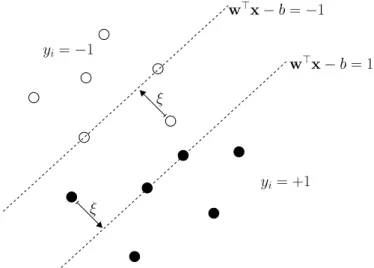
1.1 The outline of the thesis. . . 6 2.1 An illustration of the separating hyperplanes of the soft-margin SVM. . . 14 2.2 From data points to probability measures: (a) An illustration of typical

applica-tion of kernel as a high-dimensional feature map of individual data point. (b) A measure-theoretic view of high-dimensional feature map. An embedding of data point into a high-dimensional feature space can be equivalently viewed as an embedding of a Dirac measure assigning the mass 1 to each data point. (c) Generalizing the Dirac measure point of view, we can generally extend the con-cept of high-dimensional feature map to a class of probability measures. . . 19 2.3 Embedding of marginal distributions: each distribution is mapped into an

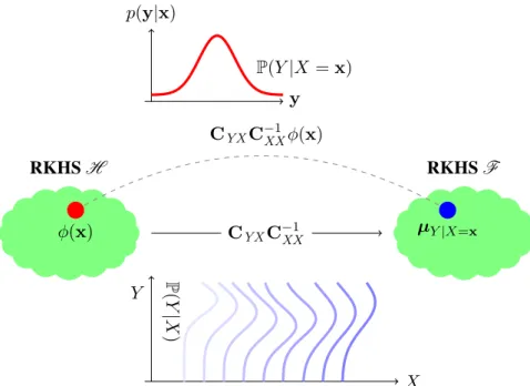
re-producing kernel Hilbert space (RKHS) via an expectation operation. It corre-sponds to a mean element in the RKHS. . . 22 2.4 From marginal distribution to conditional distribution: Unlike the embeddings

discussed in the previous chapter, the embedding of conditional distribution P(Y|X)is not a single element in the RKHS. Instead, it may be viewed as a fam-ily of Hilbert space embeddings of the conditional distributions P(Y|X = x) indexed by the conditioning variable X. In other words, the conditional mean embedding can be viewed as an operator mapping fromH toF. We will see

later in §2.4.4 that there is a natural interpretation in a vector-valued regression framework. . . 31 3.1 A 2D visualization of the ball of radiusψ(0)in the RKHS. For stationary

ker-nels, the feature map φ(x) always lie on this ball. As a result, all the kernel meansµPwill lie inside the ball. Moreover, ifk(x,y)>0for allx,y∈ X, all the feature mapsφ(x)lie in the same quadrant. Thus, the kernel meansµPwill always lie inside the ball segment. . . 49 3.2 Geometric explanation of a shrinkage estimator when estimating a mean of a

Gaussian distribution. For isotropic Gaussian, the level sets of the joint density of _θˆ_ML ₌ _X _{are hyperspheres. In this case, shrinkage has the same effect} regardless of the direction. Shaded area represents those estimates that get closer to θ after shrinkage. For anisotropic Gaussian, the level sets are concentric

ellipsoids, which makes the effect dependent on the direction of shrinkage. . . . 64 3.3 Plot ofg(γ)γ. . . 66

3.4 The comparison between the KME and its sparse approximations obtained from (3.54). . . 69 3.5 The comparison between standard estimator, µˆ and shrinkage estimator, µˆα

(withf∗ _{= 0) of the mean of the Gaussian distribution} _N₍_µ_,_Σ)_on_Rd_where

d= 1,2,3. . . 72

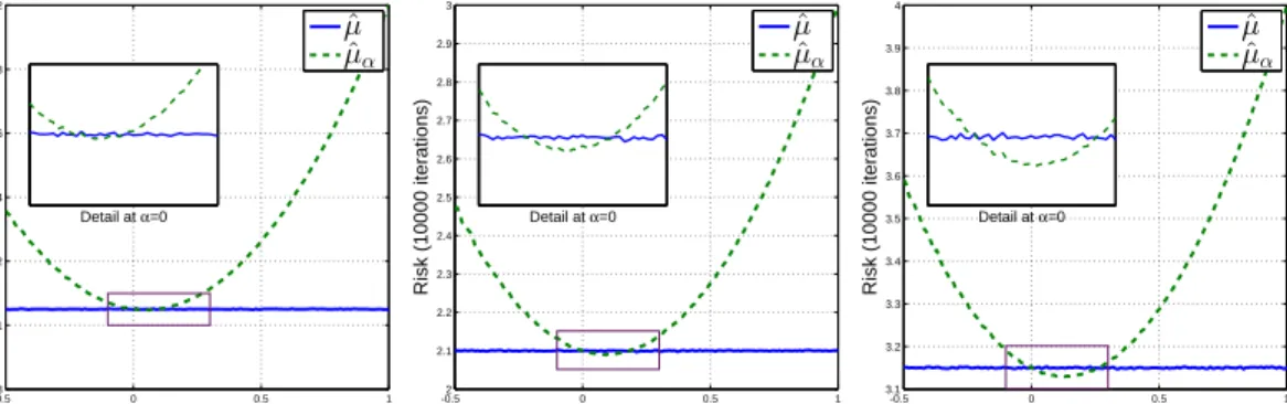
3.6 The risk comparison between standard estimator, µˆ and shrinkage estimator, ˆ

µα(withf∗ ∈ {2,(2,0)⊤,(2,0,0)⊤}) of the mean of the Gaussian distribution

(12)

LIST OF FIGURES

3.7 (a) The risk comparison betweenµˆ(KME) andµˆα˜(KMSE) whereα˜ = ˆ∆/( ˆ∆+

kf∗−µˆ_k2H). We consider whenf∗=C×k(x,·)wherexis drawn uniformly

from a pre-specified range and C is a scaling factor. (b) The probability of improvement and the risk difference as a function of shrinkage parameterα av-eraged over 1,000 iterations. As the value ofαincreases, we get more

improve-ment in term of the risk, whereas the probability of improveimprove-ment decreases as a function ofα. . . 73 3.8 The average loss of KME (left), R-KMSE (middle) and S-KMSE (right)

esti-mators with different values of shrinkage parameter. We repeat the experiments over 30 different distributions withn= 10andd= 30. . . 74 3.9 The percentage of improvement compared to KME over 30 different

distribu-tions of B-KMSE, R-KMSE and S-KMSE with varying sample size (n) and dimension (d). For B-KMSE, we calculate αusing (3.20), whereas R-KMSE and S-KMSE use LOOCV to chooseλ. . . 75 3.10 (a) For iterative algorithms, the number of iterations acts as shrinkage parameter.

(b) The iterative algorithms such as Landweber and accelerated Landweber are more efficient than the S-KMSE. (c) A percentage of improvement w.r.t. the KME, i.e.,100_×(R₋Rλ)/RwhereR andRλ denote the approximated risk of KME and KMSE, respectively. Most Spectral-KMSE algorithms outperform R-KMSE which does not take into account the geometric information of the RKHS. . . 78 3.11 The average reconstruction error of KPCA on hold-out test samples over 100

repetitions. KME represents the standard approach, whereas R-KMSE and S-KMSE use shrinkage means to perform centering. R-COSE and S-COSE di-rectly use the shrinkage estimate of the covariance operator. . . 82 4.1 (a) The decision boundaries of SVM, ASVM, and SMM. (b) the heatmap plots

of average accuracies of SMM over 30 experiments using POLY-RBF (center) and RBF-RBF (right) kernel combinations with the plots of average accuracies at different parameter values (left). . . 99 4.2 The performance of SVM, ASVM, and SMM algorithms on handwritten digits

constructed using three basic transformations. . . 99 4.3 Relative computational cost of ASVM and SMM (baseline: SMM with 2000

virtual examples). . . 100 4.4 Accuracies of four different techniques for natural scene categorization. . . 101 5.1 The graphical model describing the generative process of the framework

consid-ered in this work. The observations are sample sets whose members are drawn according to the the random distributions. . . 104 5.2 (a) The synthetic Gaussian distributions with identical mean and varying

covari-ance matrices. b the sample drawn according to the synthetic Gaussian distribu-tions. . . 106 5.3 The projection of data onto the first three principal components. Each point and

its color in the plot corresponds to the distribution shown in Figure 5.2a. . . 106 5.4 Same as Figure 5.3, but visualize the projection on the first three principal

(13)

5.5 An illustration of two types of group anomalies. An anomalous group may be a group of anomalous samples which is easy to detect (unfilled points). In this paper, we are interested in detecting anomalous groups of normal samples (filled points) which is more difficult to detect because of the higher-order statistics. Note that group anomaly we are interested in can only be observed in the space of distributions. . . 108 5.6 (a) The two dimensional representation of the RKHS of Gaussian RBF kernels.

Since the kernels depend only on x₋x′, k(x,x) is constant. Therefore, all feature mapsφ(x)(black dots) lie on a sphere in feature space. Hence, for any probability distribution P, its mean embedding µP always lies in the convex hull of the feature maps, which in this case, forms a segment of the sphere. (b) In general, the solution of OCSMM is different from the minimum enclosing sphere. (c) Three dimensional sphere in the feature space. For the Gaussian RBF kernel, the kernel mean embeddings of all distributions always lie inside the segment of the sphere. In addition, the angle between any pair of mean embeddings is always greater than zero. Consequently, the mean embeddings can be scaled,e.g., to lie on the sphere, and the map is still injective. . . 111 5.7 (a) The results of group anomaly detection on synthetic data obtained from the

OCSVM and the OCSMM. Blue dashed ovals represent the normal groups, whereas red ovals represent the detected anomalous groups. The OCSVM is only able to detect the anomalous groups that are spatially far from the rest in the dataset, whereas the OCSMM also takes into account other higher-order statistics and therefore can also detect anomalous groups which possess dis-tinctive properties. (b) The results of the OCSMM on the synthetic data of the mixture of Gaussian. The shaded boxes represent the anomalous groups that have different mixing proportion to the rest of the dataset. The OCSMM is able to detects the anomalous groups although they look reasonably normal and can-not be easily distinguished from other groups in the data set based only on an inspection. . . 114 5.8 The density functions estimated by the OCSVM and the OCSMM using the

corrupted data. . . 116 5.9 The average precision (AP) and area under the ROC curve (AUC) of different

group anomaly detection algorithms on the SDSS dataset. . . 116 5.10 The ROC of different group anomaly detection algorithms on the Higgs boson

datasets with various Higgs massesmH. . . 117 5.11 A simplified schematic diagram of the domain generalization framework. A

major difference between our framework and most previous work in domain adaptation is that we do not observe the test domains during training time. See text for detailed description on how the data are generated. . . 119 5.12 Projections of a synthetic dataset onto the first two eigenvectors obtained from

the KPCA, UDICA, COIR, and DICA. The colors of data points corresponds to the output values. The shaded boxes depict the projection of training data, whereas the unshaded boxes show projections of unseen test datasets. The fea-ture representations learnt by UDICA and DICA are more stable across test domains than those learnt by KPCA and COIR. . . 125 5.13 The leave-one-out accuracy of different methods evaluated on each subject in

the GvHD dataset. The top figure depicts the pooling setting, whereas the bot-tom figure depicts the distributional setting. . . 127

(14)

LIST OF FIGURES

5.14 The root mean square error (RMSE) of motor and total UPDRS scores predicted by GP regression after different preprocessing methods on Parkinson’s telemon-itoring dataset. The top and middle rows depicts the pooling and distributional settings; the bottom row compares the two settings. Results of linear least square (LLS) are given as a baseline. . . 128

(15)

2.1 Basic notations used throughout the thesis . . . 8 3.1 Update equations forβand corresponding filter functions. . . 66

3.2 The classification error rate of Parzen window classifier via different kernel mean estimators. The boldface represents the result whose difference from the baseline,i.e., KME, is statistically significant. . . 76 3.3 Average negative log-likelihood of the modelQon test points over 30

random-izations. The boldface represents the result whose difference from the baseline, i.e., KME, is statistically significant. . . 79 3.4 The classification accuracy of SMM and the area under ROC curve (AUC) of

OCSMM using different estimators to construct the kernel on distributions. . . 79 3.5 The average negative log-likelihood evaluated on the test set. The results are

obtained from 30 repetitions of the experiment. The boldface represents the statistically significant results. . . 80 4.1 The analytic forms of expected kernels for different choices of kernels and

dis-tributions. . . 89 4.2 Examples of some well-known kernel functions that can be used as inducing

kernels. . . 90 4.3 Accuracies (%) of SMM on synthetic data with different combinations of

em-bedding and level-2 kernels. . . 98 5.1 The AUC scores for different settings shown in Figure 5.10. . . 117 5.2 Average accuracies over 30 random subsamples of GvHD datasets. Pooling

SVM applies standard kernel function on the pooled data from multiple do-mains, whereas distributional SVM also considers similarity between domains using kernel (5.22). With sufficiently many samples, DICA outperforms other methods in both pooling and distributional settings. The performance of pooling SVM and distributional SVM are comparable in this case. . . 126 5.3 The average leave-one-out accuracies over 30 subjects on GvHD data. The

distributional SVM outperforms the pooling SVM. DICA improves classifier accuracy. . . 127 5.4 Root mean square error (RMSE) of the independent Gaussian Process regression

(GPR) applied to the Parkinson’s telemonitoring dataset. DICA outperforms other approaches in both settings; and the distributional SVM outperforms the pooling SVM. . . 128

(16)

List of Symbols

C(_X) A space of all continuous functions on_X.

C0(X) A space of all continuous functions onX which vanish at infinity.

Cb(X) A space of all bounded continuous functions onX.

L1(Rd₎ _{A space of Lebesgue integrable functions}

L2₍_Rd₎ _{A space of square integrable functions}

X A random variable taking value in_X

ϕP A characteristic function of distributionP CXX A covariance operator onX

CXY A cross-covariance operator fromXtoY

CXY_|Z A conditional cross-covariance operator ofXandY givenZ F A function space

H An RKHS of functions from_X to_R F An RKHS of functions from_Y to_R

K A Gram matrix of kernelk

L A Gram matrix of kernell

Tk An integral operator associated with kernelk

Rn(F) The Rademacher complexity of the function classF based onni.i.d. sample

φ A feature map from an input space_X to a high-dimensional feature spaceH.

P A probability measure over some input space_X

P1

+(X) A set of all probability measures defined onX.

P_b₍_X₎ A set of all finite Borel measures defined on_X.

HS(F_,H₎ A Hilbert space of Hilbert-Schmidt operators mapping fromF toH

ϕ A feature map from an input space_Y to a high-dimensional feature spaceF.

k A positive definite kernel function on_X

l A positive definite kernel function onY

(17)

Chapter

1

Introduction

I begin by giving a motivation of the thesis, its overview, and a brief outline of the subsequent chapters.

1.1

Motivations

Machine learning (ML) has played an important role in computer science and artificial intelli-gence as a mean to understand how to build a machine that is capable oflearning, and in which situations it may succeed or fail. The ultimate goal is to build an “intelligent” machine that can learn from past experience, just like human naturally do. This endeavour has already led to many successful applications of ML across different fields, ranging from astronomy and high-energy physics to robotics and causal inference. In my opinion, a key to this success lies in its multi-disciplinary nature that brings together collaborations from statisticians, neuroscientists, psychologists, cognitive scientists, and many more.

Despite the success, we are still far from understanding what an intelligent machine is. I have always been fascinated by what can be achieved through technology. The technological revolution has made our lives different from our ancestors. Better living, reliable health-care, and scientific discoveries are just tips of the iceberg. The capability of computers in performing complex tasks such as the chess-playing robots whose ability exceeds that of the human world champion and the IBM Watson that outperforms human competitors at Jeopardy has increased exponentially. But, whether or not these machines are truly intelligent remains obscure. Un-derstanding the meaning of intelligence has a great implication on what the intelligent systems can or cannot accomplish, their impact on our life, and the danger they may pose to our future. I believe one of the key ingredients to this understanding lie in theirability to learnand make future predictionabout the world.

Empirical risk minimization (ERM) is one of the most prevalent frameworks for studying the statistical learning from empirical data (Vapnik 1992). Ultimately, we are interested in finding the functional relationship between two random variablesX and Y based only on the empirical data. That is, given the independent and identically distributed (i.i.d.) random pairs

{(x1, y1), . . . ,(xn, yn)}from some unknown distribution P(X, Y)wherexi ∈ X andyi ∈ Y, the ERM finds a functionf :_{X → Y}which minimizes

b R(f) = 1 n n X i=1 ℓ(yi, f(xi)), f ∈ F (1.1)

for some function class_F. For instance, visual object recognition is one of the most important abilities we possess. In this case,ximay represent images of car andyilabelsxi by the type of car,e.g.,_Y =_{sedan,truck,sportcar,minivan,etc_}. From a collection of examples

(xi, yi), we want to findf that when applied to any image of car, returns its correct type. Since in practice we do not have access toP(X, Y), the empirical risk (1.1) is used as a surrogate to

(18)

1.1. MOTIVATIONS

its population counterpart given by

R(f) =

Z

ℓ(y, f(x)) dP(x, y), f ∈ F. (1.2)

The functionℓ:Y × Y →R+denotes a problem-specific loss function. For examples, ifY =

{0,1}, we have a classification problem and a natural choice ofℓis a 0-1 loss ℓ(yi, f(xi)) =

1f(xi)6=yi, whereas ifY =R, we have a regression problem and the common loss function is a

square lossℓ(yi, f(xi)) = (f(xi)−yi)2.

In the past decades, several efforts have been devoted to a quest for sufficient and necessary conditions under which certain problems are learnable using the ERM. This usually translates into showing that auniform convergence boundholds,i.e.,

Pn ( sup f∈F bR(f)₋R(f)> ε ) ≤g(ε, n,_F)

whereg(ε, n,_F)represents a function that depends on ε, n, and_F, and vanishes asn _{→ ∞}. This ensures that for any distributionP(X, Y), there exists a finite number of training examples nfor which the learner can generalize well to the unseen test data given that both training and test data are generated i.i.d. from the same distribution and the complexity of the function class,e.g., Rademacher complexity and VC dimension, is bounded. Although no assumption is generally made, prior knowledge aboutP(X, Y)may be used to improve learning. See,e.g., Boucheron et al.(2005) for review. Moreover, another important line of research is exploratory data analysis such as principal component analysis (PCA) in which one is interested in extracting important properties of the underlying distributionP(X)from empirical datax1, . . . ,xn.

Unlike traditional setting, the primary objects of interest in this thesis are probability dis-tributionsPi(x) over some input spaceX rather than data pointsxi themselves. The ultimate goal is then to generalize and develop learning algorithms that operate directly on a space of probability distributions. Interestingly, from a measure-theoretic point of view, many classical settings can be viewed as learning from distributions,i.e., when the data pointsxiare replaced by theDirac measures δxi which puts mass only at points xi (cf. Figure 2.2). By enriching

this perspective, the thesis investigates the feature representation of probability distribution, its empirical estimators, and general frameworks for learning on distributions based on such a rep-resentation.

1.1.1 Why Learning on Probability Distributions?

There are, in fact, many reasons why learning on probability distributions is important.

Firstly, it can be very useful in domain adaptation and transfer learning (see,e.g.,Ben-David et al.(2010), Pan et al.(2011), Pan and Yang(2010), Blanchard et al.(2011a), Muandet et al. (2013) and references therein). Several attempts have been made in generalizing the ERM to a scenario where the training and test data come from different distributions. To learn successfully in such a scenario, the algorithms need to understand how the distributions governing data gen-erating processes change across time or domains. Moreover, the training data may be obtained from distinct and heterogeneous distributions and the knowledge of the distribution of the test data may not be available during the training time.

Secondly, probability distributions are good at modeling noisy/uncertain observations. Emerg-ing technology allows us to collect a tremendous amount of data, which are usually noisy. Spe-cialized technique is needed to deal with such data. For example, gene expression data are often measured with high uncertainty. Replication, which can be costly, is required (Yang and Speed 2002) to reduce such uncertainty. Similarly, the astronomical data are always subjected

(19)

to uncertainty due to evolving nature of the objects and atmospheric disturbance. To reduce this uncertainty, the measurement is often made several times to obtain the average values ( Kirk-patrick et al. 2011,Bovy et al. 2011,Ross et al. 2012).

Moreover, in the era of “big data”, it is imperative for the machine learning algorithms to be able to extracthigh-level information contained in such data. Most of classical algorithms only make use of information from individual data points, and often neglect their interactions. In group anomaly detection, for instance, we are interested in the anomalous events that occur in the aggregate levels (Chandola et al. 2009,Póczos et al. 2011,Xiong et al. 2011b;a,Muandet and Schölkopf 2013, Guevara et al. 2014). That is, the behaviour of the group may exhibit anomalous characteristic whereas none of the points in the group is anomalous (e.g., high-energy physics). On the other hand, we may be interested in reducing the amount of data, while preserving most of the information that is necessary for successful learning. For example, we can summarize a set of data points by its average which throws away lots of information. Representing a set of data points by the distribution can capture most of the information while reducing the amount of computation required. The summary also help concealing sensitive information about individual sample,i.e., privacy-preserving (Dwork 2008).

We can interpret many problems in statistics as learning problems onempiricalprobability distributions. For example, a “statistical estimator” is essentially a function from an empirical distribution to values of certain statistics such as parameter values, independence, conditional independence, and causal relation (Lopez-Paz et al. 2015b). Statisticians often consider the “plug-in” estimators whose form are known in advance (Lehmann and Casella 1998). In con-trast, if training examples are available,learningsuch estimators allows one to impose weaker assumptions about the underlying data-generating process and may lead to “better” estimators. In many research areas, one is also interested in generalizingdomain-general knowledgewhich is domain-invariant as opposed to thedomain-specific knowledgewhich is specific to input do-main. Examples include theory of causality in cognitive science and psychology (Goodman et al. 2011).

Most importantly, probability distributions constitute more complex concept and relation intelligent entities may encounter in reality, and by studying learning problems on them I hope to gain insights into the limitations of the current intelligent systems, and how to improve them. 1.1.2 Why Kernel Mean Representation?

Previous approaches based on kernel density estimation (Póczos et al. 2013,Oliva et al. 2014), divergence measure (Póczos et al. 2011), generative model (Jebara et al. 2004b, Xiong et al. 2011a), information geometry (Amari 2010), for example, have been applied successfully for learning and statistical inference from probability distributions. In contrast, this thesis focuses on thekernel mean representation. There are multiple reasons why this representation is attrac-tive for learning framework on distributions.

First of all, kernel mean representation is very simple. It is fully characterized by a transfor-mation

P_7−→Ex∼P[k(x,·)] =:µP

wherek:X ×X →Ris a positive definite kernel function. As we can see,µPis simply a mean vector in feature space associated with the kernelk. As a result, we do not need to deal with distributions explicitly as many operations on Pcan be translated into operations onµP. The kernel meanµPcan be estimated consistently from the empirical data with provable guarantee.

Secondly, a certain class of kernel functions known ascharacteristic kernelsensures that the kernel mean representation captures all necessary information about the distribution (Fukumizu et al. 2004,Sriperumbudur et al. 2008;2010). In other words, the mapµ:P_7→µPis injective

(20)

1.2. THESIS OVERVIEW AND CONTRIBUTION

which implies that_kµP−µQkH = 0if and only ifP=Q. As a result, we can use the kernel

mean representation to define a metric over a space of probability distributions (Sriperumbudur et al. 2010). A diverse choice ofkalso gives this representation more flexibility. Most machine learning algorithms can be extended to a space of probability distributions by choosing appro-priate kernels (or approximation) of this representation (Gómez-Chova et al. 2010, Muandet et al. 2012,Guevara et al. 2014).

Next, basic operations on distributions can be performed by means of the inner product in the feature space. For example, we have EP[f(x)] = hf,µPiH for all f ∈ H. Likewise,

E_Y_|_x[g(Y)_|X =x] = _hg,_U_Y_|xiF for allg∈F whereU_Y_|_xdenotes the kernel mean

embed-ding of the conditional distributionP(Y_|X=x). Consequently, the kernel mean representation permits a probabilistic inference in a non-parametric fashion, e.g., kernel belief propagation (Song et al. 2011a), kernel Monte Carlo filter (Kanagawa et al. 2013), and kernel Bayes’ rule (Fukumizu et al. 2011).

In some applications such as testing for homogeneity from finite sample, the kernel mean representation allows one to bypass an intermediate density estimation, which is known to be difficult in high-dimensional setting (Wasserman 2006; Section 6.5). Moreover, the applica-tions of kernel mean embedding can be extended straightforwardly to non-vectorial data such as graphs, strings, and semi-groups (Gärtner 2003). Most of the previous approaches only work in standard Euclidean space.

1.2

Thesis Overview and Contribution

The major contributions of this thesis can be summarized as follows:

• Overall, the thesis introduces learning frameworks when the inputs are not just points, but probability distributions. The use of kernel mean embedding as a representation for distribution allows us to generalize many of the classical algorithms and establishes in-teresting relationships with existing frameworks. The thesis also investigates the kernel mean estimation problem.

• The thesis gives a comprehensive review on both theory and practical applications of Hilbert space embedding of probability distributions in the past years. To the best of my knowledge, this is the first comprehensive review of research in this area.

• One of the most fundamental questions is how to estimate the kernel mean effectively and efficiently from the sample, which is an essential step in the applications of kernel mean embedding. The thesis investigates this question and shows that the standard kernel mean estimator,i.e., ˆ µP := 1 n n X i=1 k(xi,·), xi∼P,

can be improved by thelinearshrinkage estimator of the formµˆα :=αf∗+ (1−α) ˆµP for someα _∈[0,1]andf∗ _∈ H. Hence, we propose a new family of estimators called

kernel mean shrinkage estimator(KMSE) and provide several theoretical guarantees. By taking the geometrical properties of RKHS into account, the thesis provide non-linear extensions by mean of spectral filtering algorithms which are quite popular in the theory of inverse problem and regularization. The proposed idea can also be used to estimate other quantities such as covariance operators.

• The thesis provides a generalization of the ERM framework to a space of distributions. That is, we observe i.i.d. sample(P₁, y1), . . . ,(Pn, yn)rather than(x1, y1), . . . ,(xn, yn).

(21)

We show that the resulting framework amounts to constructing a kernel-based learning framework over a set of distributions when each of them is represented by the kernel mean embedding. The proposed framework allows one to generalize several well-known algorithms such as kernel ridge regression and Gaussian processes to a space of proba-bility distributions. In particular, the thesis provides an extension of well-known support vector machine (SVM) to a space of probability distributions which we call a support measure machine(SMM) with theoretical insights and encouraging empirical results. In addition, the thesis provides discussions regarding connections to classical learning algo-rithms, possible extensions, and potential future directions.

• The proposed framework can also be applied in an unsupervised setting, especially for exploratory data analysis. First, the thesis provides an analysis of the feature represen-tation of distributions and illustrate this by performing PCA on distributions. Next, it presents the algorithm for group anomaly detection called one-class support measure machine (OCSMM) and provides an analysis on the connection to variable kernel den-sity estimation (VKDE). Lastly, the thesis demonstrates the proposed framework on the domain adaptation/generalization via the domain-invariant component analysis (DICA) algorithm with learning-theoretic bound.

• Last but not least, I want to point out that learning from distributions has potential applica-tions in statistics. Many problems in statistics such as hypothesis testing involve finding a function of the empirical distribution to a certain set of outputs called statistic, e.g.,

{−1,+1}indicating whether or not to reject the null hypothesis. Conventional approach is to useplug-inestimators. On a contrary, if training data is available, we maylearnsuch an estimator automatically from the data using the proposed frameworks. Preliminary re-sults have demonstrated the effectiveness of this approach in real-world applications,e.g., seeSzabó et al.(2015),Lopez-Paz et al.(2015b).

1.3

Outline of the Thesis

Figure 1.1 depicts a high-level outline of the thesis whose details can be described as follows.

Chapter 2: This chapter provides a brief literature review on the area of kernel methods and a

comprehensive review on kernel mean embedding of marginal and conditional distributions and their applications. It also provides the discussions regarding the relationships between kernel mean embeddings and other methods.

Chapter 3: This chapter addresses the kernel mean estimation problem and shows that the

standard empirical estimator of kernel mean can be improved by the shrinkage estimators. A novel class of estimators calledkernel mean shrinkage estimators(KMSEs) is proposed. Several theoretical analyses including consistency and convergence rate of estimators are also provided. Lastly, it provides extensive experimental results as evidence of the improvement of KMSEs over standard kernel mean estimator.

Chapter 4: Owing to the kernel mean embedding and its estimators, this chapter presents a

supervised learning framework on probability distributions. It first discusses thedistributional risk minimization framework and present the representer theorem for probability distributions. Next, the positive definite kernel functions for distributions based on the kernel mean embed-dings are proposed including asupport measure machine(SMM) which is a generalization of

(22)

1.3. OUTLINE OF THE THESIS Chapter 1 Introduction Chapter 2 Literature Review Chapter 3

Kernel Mean Shrink-age Estimators Chapter 4 Supervised Learning on Distributions Chapter 5 Unsupervised Learning on Distributions Chapter 6 Conclusion and Future Research Part I Part II Part III

Figure 1.1:The outline of the thesis.

well-known support vector machine (SVM) to probability measures. I also discuss its connec-tion to classical algorithms such as Parzen window classifiers. Both theoretical analysis and empirical results are also provided.

Chapter 5: This chapter demonstrates the learning framework on distributions in an

unsuper-vised setting. First, an analysis of the proposed feature representation and empirical illustration via PCA on distributions are provided. Then, the thesis presents two applications, namely, group anomaly detection and domain adaptation/generalization.

Chapter 6: This chapter concludes the thesis and gives some suggestions for future research.

(23)

Chapter

2

Literature Review

2.1

Definitions & Notations

Table 2.1 summarizes the basic notations used throughout the thesis. I use capital letters to denote random variables and lowercase letters to denote instantiations of random variables,e.g.,

Xandx. I use a bold typeface to indicate vector and matrix (or operator) quantities,e.g.,xand X. When describing the data set, I denote the total number of data points by n, and the total number of feature dimensions byd. The feature vector for the data pointiis denoted byxi, and individual feature values are denoted byxij.

The primary object of interest in this thesis is probability distribution. For a topological input space_X, I denote byPa probability measure over such a space where a Borelσ-algebra is

generated by the topology. I useϕPto denote a characteristic function ofP. LetPbe a space of all probability measuresP. For a random variableXtaking value in_X, I denote the associated probability distribution byP(X)andPX interchangeably. Given a pair of random variablesX andY, I decomposeP_intoP_X_{, which consists of the marginal distribution}_P₍_X_{), and}P

Y|X, which consists of posteriorsP(Y_|X).

For a topological space X,C(X)(resp. Cb(X)) denotes the space of all continuous (resp. bounded continuous) functions on_X. For a locally compact Hausdorff space_X,f _∈ C(_X)is said tovanish at infinity if for everyǫ > 0the set_{x : _|f(x)_{| ≥} ǫ_}is compact. I denote the class of all continuous functions on_X which vanish at infinity byC0(X). Denote byPb(X) (resp. P1

+(X)), the set of all finite Borel (resp. probability) measures defined onX.

2.2

Kernel Methods in Machine Learning

In this section, I introduce the kernel methods and the concept of reproducing kernel Hilbert space (RKHS) which form the backbone of this thesis.

2.2.1 A Kernel Trick

A solution to many classical learning algorithms such as the perceptron (Rosenblatt 1958), sup-port vector machine (SVM) (Cortes and Vapnik 1995), and principle component analysis (PCA) (Pearson 1901, Hotelling 1933b) can be expressed entirely in terms of inner product _hx,x′_i, which is basically a similarity measure between x and x′. However, a linear function class induced by this inner product is too restrictive for many real-world problems. Hence, kernel methods aim to build more flexible and powerful learning algorithms by replacing_hx,x′_iwith some other, possibly non-linear, similarity measures.

The most natural extension of_hx,x′_iis to explicitly apply a non-linear transformation:

Φ : _{X −→ F}

(24)

2.2. KERNEL METHODS IN MACHINE LEARNING

Table 2.1:Basic notations used throughout the thesis Symbol Description

X,_Y,_Z, . . . non-empty sets (input spaces)

X, Y, Z, . . . random variables taking values in_X,_Y,_Z, . . . x, y, z, . . . instantiations of random variablesX, Y, Z, . . .

v, vi a vector and itsith element

M a matrix

P a probability distribution ˆ

P an empirical distribution

ϕP a characteristic function ofP

k(x,x′) a real-valued positive definite kernel function on_{X × X}

l(y,y′) a real-valued positive definite kernel function onY × Y φ(x), ϕ(y) a feature map associated to the kernelkandl, respectively

H_,F an RKHS associated to the kernel_kand_l, respectively

CXX a covariance operator onX

CXY a cross-covariance operator fromXtoY

CXY_|Z a conditional cross-covariance operator ofXandY givenZ

into a high-dimensionalfeature space_F and subsequently evaluate the inner product there,i.e.,

k(x,x′) :=_hφ(x), φ(x′)_i. (2.2) I will refer to φ and k as a feature map and a kernel function, respectively. Likewise, we can interpretk(x,x′)as a non-linear similarity measure betweenxand x′. Consequently, we can obtain a non-linear extensions of the linear algorithms simply by substituting _hx,x′_i with

hφ(x), φ(x′₎_i_{. It is important to note that the learning algorithm remains the same: we only}

change the space in which these algorithms operate. As (2.1) is non-linear, a linear algorithm in the feature space_F corresponds to the non-linear counterpart in the input space.

Let consider a particular example of φwhen x _∈ R2_{, namely, a polynomial feature map}

φ(x) = (x2₁, x2₂,√2x1x2). Then, we have

hφ(x), φ(x′)iF =x12x′12+x22x2′2+ 2x1x2x′1x2′ =hx,x′i2. (2.3)

In other words, the new similarity measure is just the square of the dot product in_X. This result also holds more generally for ad-degree polynomial,i.e.,φmaps x _∈ RN _{to the vector}_φ_(x) whose entries are all possibledth degree ordered products of the entries ofx. In that case, we

have k(x,x′) = _hφ(x), φ(x′)_i_F = _hx,x′_id. Thus, the complexity of the learning algorithm is controlled by the complexity of φ and by increasing the degree d, one would expect that resulting algorithm will become more complex. Additional examples of how to construct an explicit feature map can be found inSchölkopf and Smola(2001; Chapter 2).

Unfortunately, evaluating k(x,x′)as above requires a two-step procedure: i) one construct the feature maps φ(x) and φ(x′) explicitly, and ii) then evaluate hφ(x), φ(x′)iF. These two

steps can be computational expensive if φ(x) lives in a high-dimensional feature space, e.g., when the degreedof the polynomial is large. Fortunately, (2.3) implies that there is an

alterna-tive way to evaluate_hφ(x), φ(x′)_i_F without resorting to constructing φ(x)explicitly if all we need is an inner product_hφ(x), φ(x′₎_i

F. That is, we can usek(x,x′) =hx,x′i2 directly. This

is an essential aspect of kernel methods, often referred to as akernel trickin machine learning community.

(25)

It turns out that there exists a general class of k which guarantee that there exists some

φ:X → F for whichk(x,x′) =hφ(x), φ(x′)iFas soon askispositive definite(cf. Definition

2.1). Since the inner product _h·,_·i is positive definite, it follows from (2.2) that kis positive definite for any choice of explicit feature mapφ.

Definition 2.1. A function k : X × X → Ris a reproducing kernel if it is symmetric, i.e.,

k(x,y) =k(y,x), and positive definite: n

X

i,j=1

cicjk(xi,xj)≥0 (2.4)

for anyn_∈Nand choice ofx1, . . . ,xn∈ X andc1, . . . , cn∈R.

Indeed a kernel function in the sense of Definition 2.1 associates to a space of functions called reproducing kernel Hilbert space (RKHS)H, hence the name_{reproducing kernel}(

Aron-szajn 1950). From this perspective, whenever we use the kernelk, we often think of acanonical feature map

k : X → H _⊂_RX (2.5)

x _7→ k(x,_·) (2.6)

whereRX denotes the vector space of functions from_X toR. An inner product inH _satisfies

thereproducing property

k(x,x′) =hk(x,·), k(x′,·)i. (2.7)

Further detail of RKHS will be provided in Section 2.2.2. Note that although we do not need to knowφ(x) =k(x,_·)explicitly, it is possible to deriveφ(_·)directly from the kernelk(see,e.g., Schölkopf and Smola(2001) for concrete examples).

The kernel trick not only results in more powerful learning algorithms, but also allows do-main experts to come up with dodo-main-specific kernel functions which can be verified easily. This leads to a number of kernel functions in various application domains (Genton 2002). In machine learning, commonly used kernels include the Gaussian and Laplacian kernels

k(x,x′) = exp −kx−x′k 2 2 2σ2 , k(x,x′) = exp −kx−x′k2 σ , (2.8)

whereσ >0is a bandwidth parameter. Compared to the Gaussian kernel, the Laplacian kernel is less sensitive to changes in bandwidth parameter. These kernels belong to a class of kernel functions called a radial basis function (RBF) kernel. Both kernels are translation invariant which form an important class of kernel functions with essential properties, see,e.g., Theorem 2.2.1

The kernel trick applies not only to real-valued random variables, but also extend to multi-variate random variables, structured data, functional data, and other domains on which positive definite kernels may be defined. A review of several classes of kernel functions can be found inGenton(2002). Hofmann et al. (2008) also provides a general review of kernel methods in machine learning.

Another characterization of symmetric positive definite kernel k is the Mercer’s theorem (Mercer 1909).

1_{The kernel}_k_{is said to be translation invariant if}_k₍

(26)

2.2. KERNEL METHODS IN MACHINE LEARNING

Theorem 2.1(Mercer’s theorem). Supposekis a continuous positive definite kernel on a com-pact setX, and the integral operatorT_k:L2(X)→L2(X)defined by

(Tkf)(·) =

Z X

k(_·,x)f(x) dx (2.9)

is positive definite,i.e.,_∀f _∈L2(X),

Z X

k(u,v)f(u)f(v) dudv ≥0. (2.10)

Then, there is an orthonormal basis{ψi}ofL2(X)consisting of eigenfunctions ofTksuch that the corresponding sequence of eigenvalues _{λi} are non-negative. The eigenfunctions corre-sponding to non-zero eigenvalues are continuous on_X andk(u,v)has the representation

k(u,v) =

∞ X

i=1

λiψi(u)ψi(v) (2.11)

where the convergence is absolute and uniform.

The condition (2.10) is known as a Mercer’s condition and the kernel functions that satisfy this condition is often referred to as Mercer’s kernels. It is important to note that Mercer’s theorem characterizes a richer class of kernel functions than the notion of positive definiteness considered previously. That is, while all Mercer’s kernels satisfy (2.2), the converse is not necessarily true. Since we are interested in the feature mapφ, throughout this thesis, we consider the positive definite kernels that satisfy (2.2). Moreover, there is an intrinsic connection between integral operatorTk, covariance operatorCXX, and Gram matrixK(Rosasco et al. 2010) (see

also Section 2.2.4).

Steinwart and Scovel (2012) studied the Mercer’s theorem in general domains in which compactness assumption on_X may not be satisfied. There is also a connection between Mer-cer’s theorem in functional analysis and Karhunen-Loève theorem in the theory of stochastic processes (Rogers and Williams 2000a;b).

When the kernel kis translation invariant,i.e.,k(x,x′) = ϕ(x₋x′),x,x′ _∈ Rd_{, we can} characterize the kernel by Bochner’s theorem (Bochner 1933).

Theorem 2.2(Bochner’s theorem). A kernelk(x,x′) = ϕ(x₋x′)onRd_{is positive definite if} and only if there exists a finite non-negative Borel measureΛonRd_{such that}

ϕ(x₋x′) =

Z

e√−1ω⊤(x−x′)dΛ(ω). (2.12)

In other words, Bochner’s theorem states thatkis the inverse Fourier transform ofΛ and the translation-invariant kernels are the class of kernel functions that have non-negative Fourier transform.

By virtue of Theorem 2.2, we can interpret the kernel k(x,x′) =ϕ(x−x′)in the Fourier domain. That is, the measureΛ determines which frequency component occurs in the kernel by putting non-negative power on each frequency ω. Note that we may normalize ksuch that

ϕ(0) = 1, in which caseΛwill be a probability measure andkcorresponds to its characteristic

function. For example, the measure Λ that corresponds to the Gaussian kernel k(x₋x′) =

e−kx₋x′_k2_/₍₂_σ2₎

is a Gaussian distribution of the form(2π/σ2₎−d/2_e−σ2_k_ω_k2_/₂

dω. For

Lapla-cian kernel k(x,x′) = e−kx−x′k/σ_{, the corresponding measure is a Cauchy distribution,} _i.e., Λ(ω) =Q_d_π₍₁₊σ_ω2

d)

(27)

As we will see later, Bochner’s theorem also allows us to characterize the kernel mean em-bedding. Similarly, the measureΛdetermines which frequency component of the characteristic function ofPoccurs in the embeddingµP. Hence, it follows from the uniqueness of the

charac-teristic function that if the support ofΛis the entireRd_,_µ

Pwill uniquely determinesP( Sripe-rumbudur et al. 2008;2010;2011a). In the context of this thesis, I prefer to think aboutΛas a filter that selects certain properties when computing the similarity measure between probability distributions_hµP,µQiH w.r.t. a certain class of distributionsP(more below).

Another promising application of Bochner’s theorem is a finite approximation of kernel function. The feature mapφof many kernel functions such as the Gaussian kernel is infinite dimensional. In which case, the construction of the Gram matrix Kwhere Kij = k(xi,xj) is required. Therefore, most kernel-based learning algorithms scale at least quadratically with the sample size, which makes them prohibitive for large-scale problems. Rahimi and Recht (2007) proposes to approximate the translation invariant kernel kby replacing the integral in (2.12) with a finite sum based on a Monte Carlo sampleω _∼ Λ. The Johnson-Lindenstrauss

Lemma (Dasgupta and Gupta 2003,Blum 2005) ensures that this transformation will preserve similarity between data points. See alsoKar and Karnick (2012), Le et al. (2013), Pham and Pagh(2013) and references therein for a generalization of this idea. Another common method to approximateKis a low-rank approximation, see,e.g.,Bach(2013) and references therein. 2.2.2 Reproducing Kernel Hilbert Space

A Reproducing kernel Hilbert space (RKHS)H _{is a Hilbert space where all evaluation}

func-tionals inH are bounded and continuous. First, I give a definition of Hilbert space.

Definition 2.2. A Hilbert space is a real (or complex) inner product space that is also a complete metric space w.r.t. the distance function induced by the inner product.

Well-known examples of Hilbert spaces include standard Euclidean space Rd_with _h_x_,_y_i the vector dot product ofxandy, a space of square summable sequencesℓ2ofx= (x1, x2, . . .)

with an inner product hx,yi = P∞_i₌₁xiyi such that the series P∞n=1|zn|2 converges, and the space of square-integrable functions L2[a, b]with inner product hf, gi =

Rb

af(x)g(x) dx. Hilbert spaces with their norm given by the inner product are examples of Banach spaces (Ledoux and Talagrand 1991). A Hilbert space is always a Banach space, but the converse need not hold because a Banach space may have a norm that is not given by an inner product, e.g., the supremum norm. This thesis will deal mostly with the embedding of distributions in the Hilbert space. Sriperumbudur et al.(2011b) has already extended the idea to a more general Banach space.

We are now in a position to give a definition of a reproducing kernel Hilbert space.

Definition 2.3. A Hilbert spaceH _{is an RKHS if the evaluation functionals are bounded,} _i.e.,

if for allx_{∈ X} there exists someC >0such that

|Fx[f]|=|f(x)| ≤CkfkH, ∀f ∈H. (2.13)

Intuitively speaking, functions in the RKHS are smooth in the sense of (2.13). This smoothness property ensures that the solution in RKHS obtained from learning algorithms will be well-behaved, i.e., small _kf −gkH implies that f(x) and g(x) are close a.e.. For example, in

classification and regression problems, it is ensured that by minimizing the empirical risk on the training data w.r.t. the functions in RKHS, we obtain a solution_fˆ_{that is close to the true solution}

f and also generalize well to unseen test data. This does not necessarily hold for functions in

(28)

2.2. KERNEL METHODS IN MACHINE LEARNING

That is, it is very easy to find a function inL2[a, b]that attains zero risk on the training data,i.e.,

overfitting.

The next theorem provides a characterization of a bounded linear operator inH_.

Theorem 2.3(Riesz representation). IfA:H _→ _R_{is a bounded linear operator in a Hilbert}

spaceH_{, there exists some}_g_A_∈H _{such that}

Af =hf, gAiH, ∀f ∈H. (2.14)

The Riesz representation theorem will be used to prove a sufficient condition for the existence of the kernel mean embedding in the Hilbert space (see Lemma 2.7). By the definition of RKHS, the evaluation functionalFx[f] =f(x)is a bounded linear operator inH. Therefore, Riesz representation theorem ensures that for anyx _{∈ X} we can find an element inH that

is a representer of the evaluation f(x). Proposition 2.4 states this result, which is called a

reproducing property.

Proposition 2.4(reproducing property). For eachx_{∈ X}, there exists a functionkx∈H such that

Fx[f] =hkx, fiH =f(x). (2.15)

The functionkxis called the reproducing kernel for the pointx. Letk : X × X → Rbe a two-variable function defined by k(x,y) := ky(x). Then, it follows from the reproducing property that

k(x,y) =ky(x) =hkx, kyiH =hφ(x), φ(y)iH, (2.16)

whereφ(x) :=kxis the feature mapφ:X →H. As mentioned earlier, we callφacanonical feature mapassociated withH _{essentially because when we apply the function}_k_(x_,_y) _{in the}

learning algorithms, the data points are implicitly represented by a function kx in the feature space. As we will see later in Section 2.3, the kernel mean embedding is defined by means of

kxand can itself be viewed as a canonical feature map of the probability distribution.

The RKHS H is fully characterized by the reproducing kernel _k. In fact, the RKHS

uniquely determinesk, and vice versa, as stated in the following theorem which is due to Aron-szajn(1950):

Theorem 2.5. For every positive definite functionk(·,·)onX × X there exits a unique RKHS, and vice versa.

The sufficient and necessary conditions for a functionk(_·,_·)to be a reproducing kernel are given in Definition 2.1. Detailed exposition of RKHS can be found inSchölkopf and Smola(2001), Berlinet and Thomas-Agnan(2004), for example.

2.2.3 Learning with Kernels

In this section I review some well-known algorithms, namely principal component analysis, support vector machine, ridge regression, and Gaussian process together with their kernelized counterparts.

Kernel Principal Component Analysis (KPCA)

Principal component analysis (PCA) is an essential tool for modern data analysis (Hotelling 1933a,Jolliffe 1986). The PCA provides a powerful mathematical tool to unravel interesting, sometimes hidden, structures that underlies a complex data set. The goal of PCA is to find a meaningful basis that “best” explains a data set in terms of the variance. That is, given a data

(29)

set_D=_{x1, . . . ,xn}wherexi ∈Rd, PCA looks for a principal componentv1inRdsuch that

the variance of the projection 1 n n X i=1  _hxi,v1i − n X j=1 hxj,v1i   2

is maximized. It is often assumed that the data setDis centered such thatPn

i=1xi =0. PCA assumes that all basis vectors _{v1, . . . ,vp} are orthonormal, i.e., hvi,vji = 0, i 6= j and

kvik2 = 1. In other words, the projection matrixV= (v1, . . . ,vp)⊤is an orthonormal matrix. Let define an×dmatrixXwhose rows correspond to data points and columns correspond to features (or variables). Then, the covariance matrixCcan be expressed in terms ofXas

C= 1

nXX

⊤_. _(2.17)

It is not difficult to show that the orthonormal basis {v1, . . . ,vp} coincides with the first p eigenvectors of C with largest eigenvalues. The eigenvalues specify the amount of variance captured by the corresponding eigenvectors. Consequently, the PCA finds the projection Vby solving the following eigendecomposition problem

CV= ΛV (2.18)

whereΛ = diag(λ1, . . . , λd)is a diagonal matrix consisting of corresponding eigenvalues. The standard PCA algorithm only gives a linear projection which can be very restrictive in many applications. As described above, the most straightforward extension of PCA to deal with non-linear relationship is to replace (2.17) with the covariance matrix in the feature space,i.e., each column of X now consists of the feature mapφ(xi). However, for infinite dimensional feature space, solving the eigenvalue problem (2.18) is no longer possible in practice.

Alternatively, one can resort to the well-known trick that conventional PCA can be refor-mulated in such a way that the data vectors appear only in the form of the scalar product (Schölkopf et al. 1998). That is, we decompose the dot product matrixX⊤X and left multi-ply by the data matrix: X⊤XU = ΛU _⇔ (XX⊤_{)(XU) = Λ(XU). As a result, the PCA}

can be performed using dot product matrix instead of covariance matrix. LetKbe a Gram ma-trix such thatKij = hφ(xi), φ(xj)i. Substituting (2.17) with the feature mapφ(xi)in (2.18), then all solutions vk lie in the span of {φ(x1), . . . , φ(xn)}. That is, there exist coefficients

α= (α1, . . . , αn)⊤such that v_k= n X i=1 αiφ(xi). (2.19)

Consequently, we can find eigenvectorvkby solving the eigenvalue problem

nλα=Kα (2.20)

for nonzero eigenvalues. Additionally, we normalize the solutionαbelonging to nonzero

eigen-values by requiring that the corresponding vectors inH _{be normalized,}_i.e.,_(v_k_·_v_k_{) = 1. This}

translates into 1 = m X i,j=1 αiαjKij =α·Kα=λk(α·α). (2.21) Given a new data pointx, the projected value ofxonto the componentvkcan be computed as Pn

i=1αihφ(xi), φ(x)i. The time complexity of eigenvalue problem (2.20) depends only on n, rather than the dimensionality d of the feature space. For large n, standard low-rank

(30)

2.2. KERNEL METHODS IN MACHINE LEARNING yi=−1 w⊤x₋_b_{= 1} w⊤x₋_b₌₋₁ ξ ξ yi= +1

Figure 2.1:An illustration of the separating hyperplanes of the soft-margin SVM.

Support Vector Machines (SVM)

Support vector machine (SVM) is one of the most successful algorithms for classification. Given a training data

D=_{(xi, yi)|xi ∈Rd, yi ∈ {+1,−1}}ni=1.

The objective of SVM is to find the maximum-margin hyperplane that separates the points havingyi = +1from those havingyi =−1.

In the following, I only give the detail of a soft-margin version of the SVM because it is widely used in many applications. Other variants of SVM formulation can be found inSchölkopf and Smola(2001). If the data in_Dare linearly separable2_{, the idea of linear SVM is to select} two hyperplanes in a way that they separate the training data and there are no points between them. In general, there could be an infinitely many of such hyperplanes. We call the distance be-tween these two hyperplane “the margin”. Among all possible hyperplanes, the SVM selects the ones to maximize this margin. Since these two hyperplanes can be described by the following equations:

w_·x₋b = 1 w·x−b = −1,

it is straightforward to show that the margin is simply2/_kw_k. Hence, maximizing margin is equivalent to minimizing_kw_kw.r.t. the constraints that the training data are correctly classified. Unfortunately, the assumption of linear separability does not hold for many real-world data. As a result, it is impossible to find such a linear hyperplane that separates the data perfectly. To relax this assumption and allow some errors to be made, the idea of soft-margin SVM is to introduce non-negative slac