Unit Root Tests are Useful for Selecting Forecasting Models
Francis X. Diebold
Lutz Kilian
Department of Economics Department of Economics University of Pennsylvania University of Michigan
First Draft: July 1997 This Draft/Print: January 18, 1999
Copyright 8 1997-1999 F.X. Diebold and L. Kilian. This paper is available on the World Wide Web at http://www.ssc.upenn.edu/~diebold/ and may be freely reproduced for educational and research purposes, so long as it is not altered, this copyright notice is reproduced with it, and it is not sold for profit.
Correspondence to: F.X. Diebold Department of Economics University of Pennsylvania 3718 Locust Walk Philadelphia, PA 19104 [email protected]
Abstract: We study the usefulness of unit root tests as diagnostic tools for selecting forecasting models. Difference stationary and trend stationary models of economic and financial time series often imply very different predictions, so deciding which model to use is tremendously important for applied forecasters. Forecasters face three choices: always difference the data, never
difference, or use a unit-root pretest. We characterize the predictive loss of these strategies for the canonical AR(1) process with trend, focusing on the effects of sample size, forecast horizon, and degree of persistence. We show that pretesting routinely improves forecast accuracy relative to forecasts from models in differences, and we give conditions under which pretesting is likely to improve forecast accuracy relative to forecasts from models in levels.
Acknowledgments: For helpful comments we thank participants at the June 1998 North
American meeting of the Econometric Society, Montreal, and the December 1998 EC2 meeting,
1. Motivation
Difference stationary and trend stationary models of the same time series may imply very
different predictions (e.g., Diebold and Senhadji, 1996). Deciding which model to use is therefore
tremendously important for applied forecasters. Rather than employing one or the other model by
default, one may use a unit root test as a diagnostic tool to guide the decision. In fact, one of the
early motivations for unit root tests was precisely to help determine whether to use forecasting
models in differences or levels in particular applications (e.g., Dickey, Bell, and Miller, 1986).
Much of the recent econometric unit root literature has focused on the inability of unit
root tests to distinguish in finite samples the unit root null from nearby stationary alternatives
(e.g., Christiano and Eichenbaum, 1990; Rudebusch, 1993). But low power against nearby
alternatives, which are typically the relevant alternatives in econometrics, is not necessarily a
concern for forecasting. It has long been asserted, for example, that the accuracy of forecasts
may be improved by employing a model in differences rather than a model in levels, if the root of
the process is close to but less than unity (e.g., Box and Jenkins, 1976, p. 192). Ultimately, the
question of interest for forecasting is not whether unit root pretests select the “true” model, but
rather whether they select models that produce superior forecasts. Surprisingly little is known
about the efficacy of unit root tests for this purpose.
The comparative merits of strategies such as “always difference,” “never difference,” or
“sometimes difference, according to the results of a unit root pretest” will in general depend on
the degree of persistence of the true process, the forecast horizon of interest, the sample size, and
the properties of the pretest. Hence the purpose of this paper is to explore systematically the
persistence, forecast horizons and sample sizes.
We focus on the univariate trending autoregressive case with high persistence, which is of
particular interest in economics and finance. Because exact finite-sample analytics appear out of
the question for the trending dynamic model of interest, we proceed by Monte Carlo simulation as
described in section 2. The results are sharp and intuitive, and are powerfully summarized by
compact response surfaces in section 3. In section 4, we meld the results into practical
prescriptions for applied work. Finally, we offer concluding remarks and directions for future
research in section 5.
2. Experimental Design
Here, as always, there is inescapable tension in experimental design. On the one hand, we
want to examine a wide enough range of data-generating processes (DGPs) such that the results
shed light on the behavior of alternative methods and on a range of empirically-relevant situations.
Clearly, we will want to examine a range of forecast horizons, degrees of persistence, and sample
sizes. On the other hand, it is crucial that the DGPs examined be simple and their range small
enough to promote manageable and interpretable Monte Carlo analysis.
Use of a first-order autoregressive DGP, with differing degrees of persistence
corresponding to different autoregressive parameter values, represents an appealing compromise.
If, however, the analysis is to provide meaningful recommendations for applied work, we view the
inclusion of a time trend as crucial. Trending behavior is routinely present in economic and
financial series and increases the amount of bias in the least squares estimator of autoregressive
parameters, which has important implications for the performance of the alternative strategies of
(yt&a&b t) ' D(y
t&1&a&b (t&1)) % gt
gt iid- N(0, F2), yt ' k 1 % k2t % Dyt&1 % gt, k1 ' a(1&D) % Db k2 ' b(1&D). yt ' T t % xt, Tt ' a % bt
Hence we examine a trending AR(1) process of the form
t = 1, 2, ..., T. We can rewrite the process as
where
and
Perhaps more intuitively, we can express the process in components form as the sum of a linear
trend and an AR(1) process,
xt ' Dx
t&1 % gt.
and
When D = 1 the process is a random walk with drift b, and when D<1 the process is covariance stationary AR(1) deviations from a linear trend with slope b.
We parameterize the process to be consistent with U.S. postwar quarterly real GNP data
by setting a = 7.3707, b = 0.0065, and F = 0.0099. This parameterization is likely to be representative for many other trending macroeconomic time series as well. We examine
and , which includes
D,{0.5,0.9,0.97,0.99,1} T0{25, 30:10:80, 100:20:180 , 200:40:1000 }
relevant degrees of persistence and sample sizes for annual, quarterly, monthly, weekly, and daily
data.
We compare the performance of three forecasting models: AR(1) in levels with linear
deterministic trend (L, for “levels”), random walk with drift (D, for “differences”), and the model
suggested by Dickey-Fuller unit root pre-tests using 5 percent finite-sample critical values (P, for
“pretest”). For all models, the estimation method is ordinary least squares (OLS). The common
objective is to forecast the level of the series at horizons, h, ranging from 1 to 100 periods ahead.
Using common random numbers across models, we evaluate the performance of each model by its
unconditional prediction mean squared error (PMSE) in 20,000 Monte Carlo trials. For each
value of D, we calculate the ratios PMSE(D)/PMSE(L), PMSE(D)/PMSE(P), and PMSE(P)/PMSE(L) for all combinations of h and T.
3. Results
PMSE(D)/PMSE(L), PMSE(D)/PMSE(P), and PMSE(P)/PMSE(L), for all combinations of
forecast horizon (h) and sample size (T). In particular, for each value of D, we show the relative PMSE as a function of h and T. We present unsmoothed response surfaces, because they are
quite smooth already and readily interpretable without additional smoothing.
D vs. L
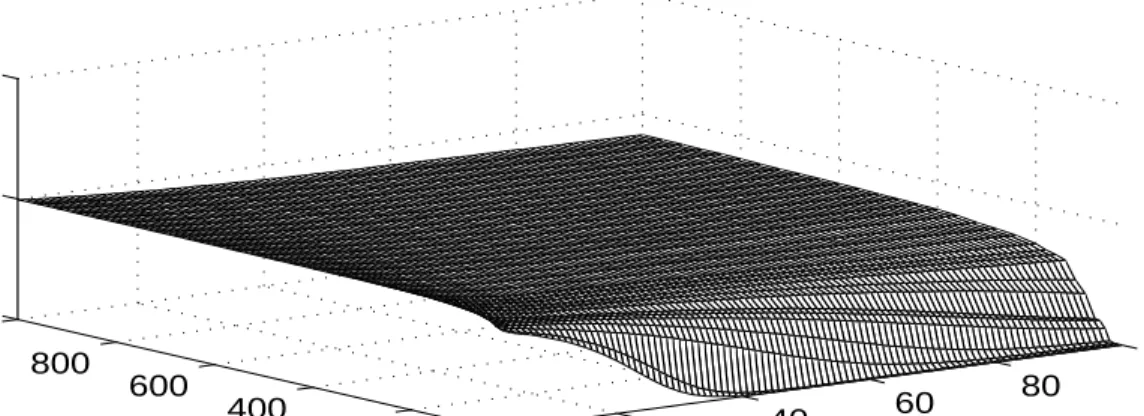
Figure 1 makes clear that neither D nor L dominates always; the relative forecast accuracy
in general depends on , h and T. Not surprisingly, forD D'1 the D model is uniformly more accurate than the L model, because in that case D is the true model. The ratio
PMSE(D)/PMSE(L) drops toward 0 as the forecast horizon h grows (for fixed sample size, T).
This happens because the distortions resulting from the Dickey-Fuller small-sample bias, which
plague the L model, are magnified as h grows. This effect, of course, is most pronounced for
smaller sample sizes, for which the Dickey-Fuller bias is greatest. As a result, for fixed forecast
horizon h, the ratio PMSE(D)/PMSE(L) drops toward 0 as T declines.
In contrast, for roots smaller than unity, D is false and would not be expected to dominate
L always. That expectation is confirmed. For D'0.99, for example, for sample sizes in excess of 600, forecasts from L are marginally more accurate than those from D. The D model forecast is
least accurate for large h. This is to be expected, as the error resulting from the false imposition
of a unit root is compounded with rising h. In contrast, small-sample bias is of little concern for
such large samples, and L is quite accurate. Nevertheless, for smaller sample sizes, forecasts from
D continue to be more accurate than forecasts on the basis of the biased estimator associated with
L, especially for long forecast horizons.
1 The problem is that for processes with large roots there is a non-negligible probability in
small samples of drawing an explosive estimate. As a result, using L, we occasionally encounter predictions based on “outlier” explosive models, which have extremely large prediction errors and dominate the PMSE. Typically in such cases the forecast dives toward minus infinity, due to a slightly negative estimated trend coefficient and an estimated root in excess of unity. As a result, the PMSE does not improve at long horizons as the process reverts back to its mean, as one might have expected, because the effect of explosive forecasts on the PMSE obviously worsens for longer horizons. The problem does not arise in D because of the imposition of a unit root. While the PMSE of D worsens for longer forecast horizons, as one would expect, the extent to which its PMSE deteriorates is dwarfed by the PMSE of L, which is inflated by the occasional explosive outliers. The net result is a ratio of PMSE(D)/PMSE(L) that approaches zero. In light of these phenomena, we also experimented with a mixed strategy (M), in which we used the L forecast unless the L forecast was explosive, in which case we replaced the L forecast with the D forecast. As expected, the small-sample forecast accuracy of M was much better than that of L, but, interestingly, the modification did not affect our qualitative results.
the process declines. For D'0.97, the ratio PMSE(D)/PMSE(L) exceeds 1 over much of the parameter space and is highest when both T and h are large. For small T and large h, however,
the ratio still tends to approach zero. The poor relative performance of the L model for small T
and large h is not only due to small-sample bias. In addition, the PMSE of L is inflated by
occasional explosive estimates, resulting in absurd forecasts, especially at long forecast horizons.1
In contrast, the constraint implicit in D renders its forecasts more consistently reasonable, even
when D is incorrect.
We also find that for small T, the ratio PMSE(D)/PMSE(L) decreases in h, whereas for
large T it increases in h. This reversal makes sense. For small T, the loss in forecast accuracy
from poor estimates of L is much greater than the loss from inappropriately using the model in
differences, and the tradeoff worsens as h increases. In contrast, for large T, the forecast from L
is increasingly more accurate (because the least squares estimator is consistent), whereas using the
model in differences (and thereby imposing a unit root) introduces a systematic distortion in
The results forD'0.9 are similar, but even more pronounced. Differencing continues to improve forecast accuracy for small and moderate sample sizes, but as the persistence of the
process declines, the gains are limited to increasingly smaller sample sizes. At the same time, for
larger sample sizes, L becomes increasingly more accurate than the model in differences,
especially as the forecast horizon increases.
It is interesting to note that in the case of D'0.9, as well as several cases discussed later, for large T the ratio PMSE(D)/PMSE(L) (and later PMSE(D)/PMSE(P)) approaches 2 as h
grows. This phenomenon occurs when T is large enough so that the parameters of the L model
are estimated precisely (or, equivalently, for T large enough so that the unit root null hypothesis
tends to be rejected correctly, and the resulting trend stationary model is estimated precisely).
The explanation is simple: in population, when D<1, the long-horizon forecast error from L is approximately the unconditional variance of the process, var(yt), whereas the long-horizon
forecast error from the model in differences is approximately var(yt%h&y , which approximately
t)
equals twice the unconditional variance of the process. Appearance of these population results in
the finite-sample Monte Carlo results requires a sample large enough to facilitate precise
estimation and powerful unit root testing.
Finally, for D'0.5, the L model uniformly dominates the D model. What makes this case interesting is the emergence of a “ridge” in the response surface for small T. The height of the
ridge steadily increases in h. We do not yet have an explanation for the ridge.
Taken as a whole, the D vs. L results appear driven by the fact that differencing provides
insurance against problems due to Dickey-Fuller bias and explosive root problems, at a cost.
cost. Elsewhere in the parameter space, however, the situation is reversed. As a rule of thumb,
the results suggest that one is better off differencing if the sample size is small or moderate and
the process appears highly persistent, and conversely. Note in particular that the “we don’t know
and we don’t care” view is explicitly refuted: although the trend-stationary vs. difference
stationary distinction is not important in some contexts; it most definitely makes a difference for
forecasting. Moreover, the best forecasting model is not necessarily the true model; the ability of
a unit root pretest to select a good forecasting model is distinct from its ability to select the true
model. The fact that neither D nor L dominates uniformly suggests that unit root pretests may
help to improve forecast accuracy. We now explore this possibility in detail.
D vs. P
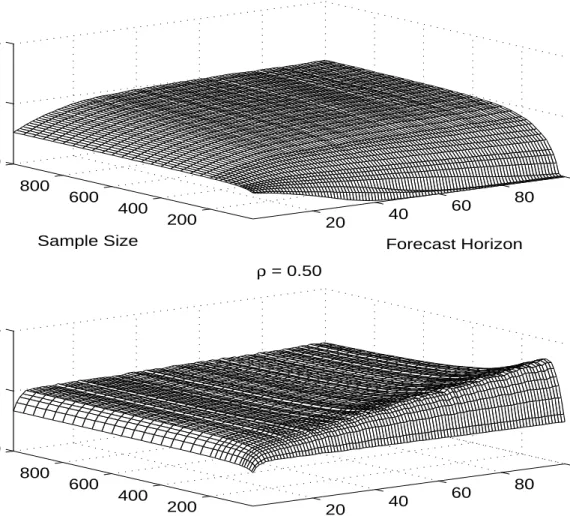
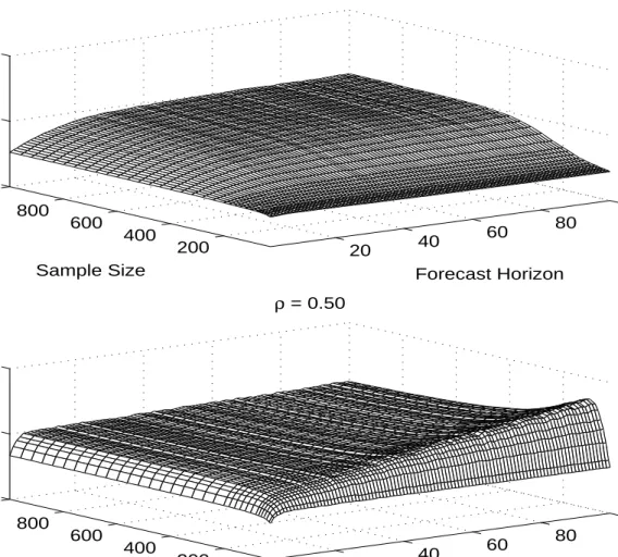
Figure 2 makes clear that the pre-testing strategy dominates that of routinely differencing
the data for almost all sample sizes and forecast horizons. The reason is that our pretest takes the
unit root hypothesis as its null. For alternatives close to the unit root null, the power of the
pre-test is low, so the pre-pre-test model reduces to the model in differences. Hence, P performs much
like D did in Figure 1, when that model is a good approximation. On the other hand, for
processes with roots far from the unit root null, the Dickey-Fuller test is bound to find strong
evidence against the null, in which case the pre-test model reduces to L, which we know to be
much more accurate than D when persistence is low.
In particular, we find that for D'1, when D is the true model, the pre-test is unlikely to reject the model in differences, resulting in a PMSE(D)/ PMSE(P) ratio very close to 1. Similar
results hold forD'0.99. For D'0.97, P begins to exhibit important advantages over D. For small T, the test lacks power and rarely rejects, so P and D coincide, and PMSE(D)/PMSE(P) is
effectively 1 regardless of h. As T grows, the test rejects the unit root null more often, yet the
ratio PMSE(D)/PMSE(P) remains close to 1. The reason is that, at least for small h, the PMSE
for a highly persistent process in levels tends to be close to that of the equivalent model in
differences. Because for large T the L model will be estimated rather precisely, the resulting
forecast is about as accurate as that for the D model. In contrast, for both T and h large, the P
forecast is considerably more accurate than the D forecast. This outcome is reflected in
PMSE(D)/ PMSE(P) ratios in excess of 1. The reason is that for long horizons the false
imposition of a unit root (which is of little consequence for short horizons) becomes a liability.
This tendency becomes even more apparent forD'0.9. Only for very small T, the relative accuracy of D and P remains similar. In general, the P model is much more accurate than the D
model. Finally, consider the process with D'0.5. In Figure 1 we showed that the loss in forecast accuracy from falsely adopting the model in differences is very high for D'0.5. However, the Dickey-Fuller pre-test has considerable power against this distant alternative and almost always
rejects the model in differences. Hence, P and L tend to coincide, and the PMSE(D)/PMSE(P)
results in Figure 2 are almost identical to those in the corresponding panel of Figure 1 for
PMSE(D)/PMSE(L).
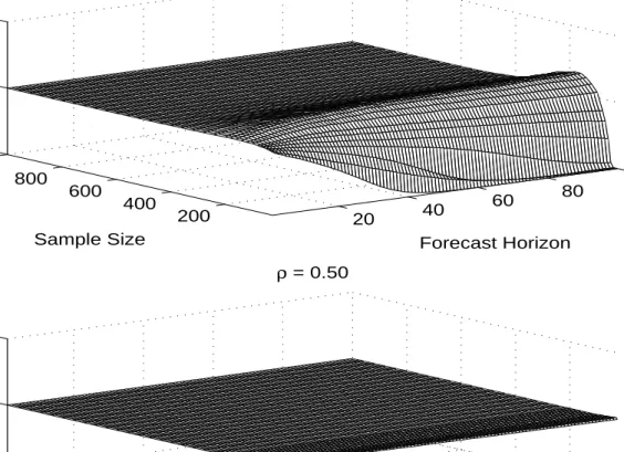
P vs. L
In Figure 3 we directly compare P and L. For D'1, pre-testing gives similar results to differencing. Not surprisingly, pre-testing uniformly dominates the levels model. Similar results
hold, at least for small and moderate sample sizes, for D'0.99. Figure 3 indicates that pre-test based forecasts are about as accurate as the level forecasts when D'0.5. The most interesting
results are for the intermediate region of D'0.97and D'0.9. For small and moderate T and large h, Figure 3 shows evidence of a “ridge” on the response surface for D'0.9. That ridge flattens and widens for D'0.97, as the accuracy of the pre-test model improves. Evidently those are cases for which we would like to have rejected the unit root null hypothesis, but did not.
Although the root is far enough from the unit circle, and the sample size (albeit small) is large
enough for the levels models to be reasonably accurate, the Dickey-Fuller test is not powerful
enough to detect the absence of a unit root. This observation suggests that more powerful unit
root tests such as the DF-GLS test of Elliott et al. (1996) could be used to flatten the ridge and to
improve forecast accuracy. However, it is not obvious that more powerful tests would be
beneficial in all regions of the parameter space. As we showed earlier, in some cases using
incorrectly the model in differences rather than the correct model in levels will actually improve
forecast accuracy, so more powerful unit root pre-tests may actually worsen forecast accuracy in
those regions. More research is needed to quantify these tradeoffs.
A Summary Assessment
Taken as a whole, the results cast the pretesting strategy in a favorable light. P dominates
D uniformly, which makes clear that the Box-Jenkins strategy of routinely differencing to achieve
stationarity is not to be recommended for constructing forecasting models. P does not dominate
L uniformly, but it nevertheless dominates over much of the design space, which similarly casts
doubt on a strategy relying on asymptotics by routinely specifying forecasting models in levels.
4. Some Practical Advice
Given the wide range of sample sizes and forecast horizons, it is difficult to translate the
GNP may not be representative for other frequencies. We therefore repeated the simulation
exercise for selected sample sizes and forecast horizons for DGPs specifically chosen to be
representative for each frequency. As the pre-testing strategy clearly dominates differencing, we
focus on the choice between pre-testing and routinely forecasting on the basis of the level model.
Table 1 summarizes the simulation design for each frequency. The quarterly DGP based
on U.S. real GNP is identical to the DGP defined in section 2. The annual DGP is based on 125
observations for U.S. per capita real GNP as defined in Diebold and Senhadji (1996). The daily
DGP is based on the Dow Jones stock price index for 1/1/74-4/2/98, and the monthly DGP is
based on U.S. industrial production index (DRI code: IP) for the post-war period.
For annual data (say, T = 40-160 and h = 1-100), we find that pre-testing unambiguously
improves forecast accuracy for all forecast horizons and sample sizes if the root of the DGP is
0.97 or higher. For D'0.9, pre-testing still improves forecast accuracy for sample sizes as high as 70, but does not perform as well as the L model in larger samples. For D'0.5, the two models are tied. In practice, this result suggests using pre-tests for data sets of up to 70 annual
observations, and for all larger sample sizes, provided the process is likely to be highly persistent.
In the remaining cases, the L model is preferred.
For quarterly data (say, T = 80-200 and h = 1-16), the P model is more accurate for all
forecast horizons and sample sizes, provided the root of the process is 0.97 or higher. For
the level model is uniformly more accurate, and for the models are tied. We
D'0.9, D'0.5
conclude that pre-testing should be used for all processes with roots of 0.97 or higher, and the L
model for processes with smaller roots.
2
These differences in dominant roots across sampling frequencies make sense when viewed in terms of the implied half-life of the response to an innovation (see Caner and Kilian, 1998).
for D'1and for D'0.99 for all forecast horizons and sample sizes considered. For D'0.97and however, the L model is at least as accurate as the P model, and for the two
D'0.9, D'0.5
methods are tied. This finding suggests that pre-testing is useful only for processes with roots of
0.99 or higher, and in all other cases the L model will be more accurate.
For daily data (say, T = 360-720 and h = 1-90), pre-testing only improves forecast
accuracy uniformly for D'1. For D'0.99 the performance is mixed, with the P model being more accurate for sample sizes of fewer than 600 days at all horizons. For larger sample sizes, the
L model is slightly more accurate at long forecast horizons, and roughly as accurate as the P
model at shorter horizons. For D'0.97 the L model is uniformly more accurate. For D'0.9 the L model is slightly more accurate for small T, especially for T < 500, except at very short
horizons. For larger sample sizes the differences vanish. For D'0.5 the two methods are tied. This finding suggests that pre-testing is useful for forecasting daily data only if the data are very
persistent with roots of 0.99 or higher. For other applications, the L model is likely to be more
appropriate.
Our advice may appear to be circular in that it often depends on knowledge of the true
root. In practice, however, OLS point estimates of the roots for quarterly macroeconomic data
are typically in excess of 0.97, estimates for monthly data are in excess of 0.99 and estimates for
daily data are well in excess of 0.99.2 Moreover, the presence of small-sample bias suggests that
pre-testing is recommended for virtually all forecasting exercises involving trending macroeconomic
data.
5. Concluding Remarks and Directions for Future Research
Difference stationary and trend stationary models of the same series may imply very
different predictions. Deciding which model to use thus is tremendously important for applied
forecasters, and unit root pre-tests may provide a formal criterion for deciding whether to
difference the data. However, very little is known about the usefulness of unit root tests as
diagnostic tools for selecting a forecasting model. In an effort to remedy this situation, we
conducted a Monte Carlo study in which we explored systematically the extent to which
pre-testing for unit roots improves forecast accuracy in a canonical AR(1) model with trend, for a
variety of sample sizes, forecast horizons, and degrees of persistence. We found strong evidence
that pre-testing improves forecast accuracy relative to routinely differencing the data. We also
characterized in detail under what conditions pre-testing is likely to improve forecast accuracy
relative to forecasts from models in levels and provided some practical advice.
Our work builds on, and complements, a small literature dating back almost a decade.
Stock (1990) finds in a particular application that model specification in levels vs. differences
matters little, but points out that in general it will. Some preliminary evidence in favor of
pre-testing is presented in Campbell and Perron (1991) who study 1-step-ahead and 20-step-ahead
forecasts made using autoregressive models. They show that one loses little by pretesting relative
to using the true model, and sometimes one actually gains. In their study, autoregressive models
in levels do best for series that are near white noise, while autoregressive models in differences do
Perron, explores longer forecast horizons. He compares level and difference stationary models,
but does not discuss pre-testing. Neither do Franses and Kleibergen (1996), who study the
out-of-sample forecasting accuracy of trend stationary and difference stationary models for the
Nelson-Plosser data set.
The extant work most closely related to ours is Stock (1996) and Stock and Watson
(1998). Stock (1996) provides theoretical arguments in favor of pre-testing from a local-to-unity
asymptotic perspective and presents some Monte Carlo evidence for the AR(1) model without
trend. In recent contemporaneous and independent work, Stock and Watson (1998) provide a
comprehensive empirical study of the out-of-sample accuracy of macroeconomic forecasting
models; one of their conclusions is that autoregressive models based on unit root pre-tests tend to
perform well.
Our Monte Carlo results complement and strengthen both the largely theoretical work of
Stock (1996) and the purely empirical work of Stock and Watson (1998). Our analysis is closer
in spirit to Stock’s, but there are important differences. Stock focused narrowly on documenting
problems in long horizon forecasting from models with roots close to unity. Moreover, he did not
consider models with trend, and he fixed the ratio h/T in his Monte Carlo analysis. Our analysis,
in contrast, is wider in scope. It includes a grid of alternative values of , h and T, correspondingD to applications of autoregressive forecast models using daily, weekly, monthly, quarterly, and
annual data. To the extent that results can be compared directly, ours and Stock’s tend to agree;
however, we find stronger evidence in favor of pre-testing than Stock (1996), reflecting the
greater importance of small-sample bias in models with trends.
3 In addition, it would be of interest to explore tests that take L rather than D as the null
hypothesis (see Kwiatkowski, Phillips, Schmidt and Shin, 1992, and Leybourne and McCabe, 994). Pretest procedures based on such unit root tests might be expected to dominate L for the same reason that the Dickey-Fuller pretest dominates D. This optimism is tempered, however, by recent work of Caner and Kilian (1998), which documents large finite-sample size distortions of such tests and the impossibility of fixing them by conventional means.
AR(1) data generating process, the results by necessity are tentative, and there are many obvious
but nevertheless important variations on the applications considered in this paper. For example,
we chose to focus on just one of many pre-tests for unit roots, and we ignored asymptotic
refinements of unit root tests based on bootstrap theory (e.g., Nankervis and Savin, 1996).
Moreover, Stock (1996) showed that the asymptotically more powerful DF-GLS test of Elliott et
al. (1996) may further improve forecast accuracy. Our analysis confirmed that there are
important potential advantages to the use of more powerful unit root tests in some regions of the
parameter space, but it also showed that low power in some cases may improve forecast accuracy.
This finding suggests that there are likely to be tradeoffs between different unit root pre-tests in
terms of their power properties. Working with daily data, for example, may call for different unit
root tests than working with annual data. Future research will have to quantify these tradeoffs.3
Another limitation of our Monte Carlo analysis is the greatly simplified lag structure of the
data generating process. Further research is required to verify the robustness of our findings in
models with richer dynamics. We also deliberately ignored the issue of lag order uncertainty at
this stage of the analysis. Future work will have to address the fact that the population model is
unknown in practice and may not even be of finite lag order. Appropriate data-based lag order
selection procedures for the class of ARMA(p,q) models are discussed for example in Ng and
A third limitation of our analysis is our focus on univariate models. Univariate models are
of central interest in many applications and often have proved superior to multivariate forecasting
models, but they are not the only model in use. For example, Stock (1990, 1994) notes that
results for univariate models do not bear directly on macroeconomic forecasting, which is
typically multivariate. Future research undoubtedly will have to include vector valued processes.
While the standard ADF test used in this paper is widely used as a pre-test for vector
autoregressions, a similar analysis for multivariate cointegration tests would be useful. One would
conjecture that imposing cointegration in small samples ought to improve forecast accuracy,
whether or not cointegration holds exactly. However, there is reason to believe that imposing
cointegration may be less important than commonly thought. For example, Christoffersen and
Diebold (1998) show that when forecasting cointegrated systems at long horizons, imposing the
correct order of integration is crucial, but imposing cointegration is not.
A fourth extension would be to allow for endogenously selected deterministic trend breaks
under the alternative. In particular, piece-wise linear deterministic trend models may forecast
more accurately than linear models. The ADF test considered in this paper does not allow for
trend breaks, but tests like those developed in Zivot and Andrews (1992) do. Moreover,
alternative procedures for the simultaneous determination of the trend model and of the order of
integration have been proposed for example by Phillips and Ploberger (1994).
A fifth extension would be to explore alternative estimators. Canjels and Watson (1997)
document that for processes with roots close to unity, the feasible GLS estimator of Prais and
Winsten (1954) provides the best estimates of the trend coefficient. Given the obvious
forecast accuracy of the Prais-Winston estimator to the OLS estimator used in this paper would
be useful. In addition, it would be worthwhile to study bias-corrected OLS forecasts. Our
simulation results are consistent with the view that much of the advantage of falsely imposing a
unit root in borderline stationary processes is due to the elimination of OLS small-sample bias. A
natural conjecture is that the mean squared error of forecasts from trend stationary models may be
improved by replacing the OLS autoregressive coefficient estimates by bias-corrected coefficient
estimates. Such corrections have been used successfully in the closely related area of impulse
response analysis. For example, Andrews and Chen (1994) report that approximate median bias
corrections for univariate autoregressive models may reduce the mean squared error of impulse
response estimates for at least some parameter ranges and horizons. Alternative bias corrections
based on the mean bias of the autoregressive coefficient estimates have been explored by
Rudebusch (1993) and Kilian (1998) based on work by Shaman and Stine (1988) and Pope
(1990).
A sixth extension would be to examine the robustness of the results to structural change,
in light of recent work by Clements and Hendry (1998) indicating that certain specifications may
be relatively more robust to structural change than others.
A final extension, and perhaps the most novel and interesting in our view, would be to
consider unit root test sizes other than 5 percent, and to determine how the performance of P
relative to D and L varies with test size. In particular, it should be possible to tune the test size to
optimize the performance of P. The present fairly stringent size of 5 percent leads to domination
of D by P, because the pretest selects D except when there is strong evidence against D, but fails
intact the domination of D by P, but could bring us closer to a similar domination of L by P. At
any rate, there is certainly no reason to think that the arbitrary size of 5 percent is necessarily
close to optimal. Hence our results on the generally good performance of the pretesting strategy
are conservative -- some simple additional tuning could cast the pretest strategy in an even more
References
Andrews, D.W.K. and Chen, H.-Y. (1994), “Approximately Median-Unbiased Estimation of Autoregressive Models,” Journal of Business and Economic Statistics, 12, 187-204.
Box, G.E.P. and Jenkins, G.W. (1976), Time Series Analysis, Forecasting and Control, Second Edition. Oakland, CA: Holden-Day.
Campbell, J.Y. and Perron, P. (1991), “Pitfalls and Opportunities: What Macroeconomists Should Know About Unit Roots,” in O. Blanchard and S. Fischer (eds.), NBER Macroeconomics Annual, 1991. Cambridge, Mass.: MIT Press.
Caner, M. and Kilian, L. (1998), “Size Distortions of Tests of the Null Hypothesis of Stationarity: Evidence and Implications for Applied Work,” Manuscript, Department of Economics, University of Michigan.
Canjels, E. and Watson, M. (1997), “Estimating Deterministic Trends in the Presence of Serially Correlated Errors,” Review of Economics and Statistics, 79, 184-200.
Christiano, L.J. and Eichenbaum, M. (1990), “Unit Roots in Real GNP: Do we Know and do we Care?,” Carnegie-Rochester Conference Series on Public Policy, 32, 7-82.
Christoffersen, P.F. and Diebold, F.X. (1998), “Cointegration and Long-Horizon Forecasting,”
Journal of Business and Economic Statistics, 16, 450-458.
Clements, M.P. and Hendry, D.F. (1998), “How to win Forecasting Competitions in Economics,” Manuscript, Economics Department, Warwick University, and Nuffield College, Oxford.
Cochrane, J.H. (1991), “A Comment on Campbell and Perron,” in O. Blanchard and S. Fischer (eds.), NBER Macroeconomics Annual, 1991. Cambridge, Mass.: MIT Press.
Dickey, A.D., Bell, W.R. and Miller, R.B. (1986), “Unit Roots in Time Series Models: Tests and Implications,” The American Statistician, 40, 12-26.
Diebold, F.X. and Senhadji, A.S. (1996), “The Uncertain Unit Root in Real GNP: Comment,”
American Economic Review, 86, 1291-1298.
Elliott, G., Rothenberg, T.J., and Stock, J.H. (1996), “Efficient Tests for an Autoregressive Unit Root,” Econometrica, 64, 813-836.
Franses, P.H. and Kleibergen, F. (1996), “Unit Roots in the Nelson-Plosser Data: Do They Matter for Forecasting?,” International Journal of Forecasting, 12, 283-288.
Kilian, L. (1998), “Small-Sample Confidence Intervals for Impulse Response Functions,” Review of Economics and Statistics, 80, 218-230.
Kwiatkowski, D., Phillips, P.C.B., Schmidt, P., and Shin, Y. (1992), “Testing the Null Hypothesis of Stationarity Against the Alternative of a Unit Root,” Journal of Econometrics, 54, 159-178.
Leybourne, S.J. and McCabe, B.P.M. (1994), “A Consistent Test for a Unit Root,” Journal of Business and Economic Statistics, 12, 157-166.
Nankervis, J.C. and Savin, N.E. (1996), “The Level and Power of the Bootstrap t Test in the AR(1) Model with Time Trend,” Journal of Business and Economic Statistics, 14, 161-168.
Ng, S. and Perron, P. (1995), “Unit Root Tests in ARMA Models with Data Dependent Methods for the Selection of the Truncation Lag,” Journal of the American Statistical Association, 90, 268-281.
Phillips, P.C.B. and Ploberger, W. (1994), “Posterior Odds Testing for a Unit Root with Data-Based Model Selection,” Econometric Theory, 10, 774-808.
Prais, S.J., and Winsten, C.B. (1954), “Trend Estimators and Serial Correlation,” Cowles Foundation Discussion Paper No. 383.
Pope, A.L. (1990), “Biases of Estimators in Multivariate Non-Gaussian Autoregressions,”
Journal of Time Series Analysis, 11, 249-258.
Rudebusch, G.D. (1993), “The Uncertain Unit Root in Real GNP,” American Economic Review, 83, 264-272.
Shaman, P. and Stine, R.A. (1988), “The Bias of Autoregressive Coefficient Estimators,” Journal of the American Statistical Association, 83, 842-848.
Stock, J.H. (1990), “Unit Roots in Economic Time Series: Do We Know and Do We Care? A Comment,” Carnegie-Rochester Conference Series on Public Policy, 32, 63-82.
Stock, J.H. (1994), “Unit Roots, Structural Breaks, and Trends,” in R. Engle and D. McFadden (eds.), Handbook of Econometrics, Volume 4. Amsterdam: North-Holland.
Stock, J.H. (1996), “VAR, Error Correction, and Pretest Forecasts at Long Horizons,” Oxford Bulletin of Economics and Statistics, 58, 685-701.
Models for Forecasting Macroeconomic Time Series,” Manuscript, Kennedy School, Harvard University, and Woodrow Wilson School, Princeton University.
Zivot, E. and Andrews, D.W.K. (1992), “Further Evidence on the Great Crash, the Oil Price Shock, and the Unit Root Hypothesis,” Journal of Business and Economic Statistics, 10, 251-270.
Table 1
Data Generating Processes
Frequency a b F DGP based on:
Annual -6.0674 0.0173 0.0500 U.S. per capita
real GNP
Quarterly 7.3707 0.0065 0.0099 U.S. real GNP
Monthly 3.3654 0.0024 0.0105 U.S. industrial
production
Daily 5.1126 0.0004 0.0095 Dow Jones
stock price index
Notes: The DGP is (yt&a&b t) ' D(y , where is the standard error of .
Figure 1a: PMSE(D)/PMSE(L)
20 40 60 80 100 200 400 600 800 10000 1 2 Forecast Horizon ρ = 1.00 Sample Size D/L 20 40 60 80 100 200 400 600 800 10000 1 2 Forecast Horizon ρ = 0.99 Sample Size D/L 20 40 60 80 100 200 400 600 800 10000 1 2 Forecast Horizon ρ = 0.97 Sample Size D/LSOURCE: 20,000 Monte Carlo trials based on DGP yt =(a−aρ+bρ)+ −(b bρ)t+ρ yt−1 +εt,
where ε ~ N( , .0 0 012)
Figure 1b: PMSE(D)/PMSE(L)
20 40 60 80 100 200 400 600 800 10000 2 4 Forecast Horizon ρ = 0.90 Sample Size D/L 20 40 60 80 100 200 400 600 800 10000 2 4 Forecast Horizon ρ = 0.50 Sample Size D/LSOURCE: 20,000 Monte Carlo trials based on DGP yt =(a−aρ+bρ)+ −(b bρ)t+ρ yt−1 +εt,
where εt ~ N( , .0 0 01 )
2
, a=7 3707. , b=0 0065. .
Figure 2a: PMSE(D)/PMSE(P)
20 40 60 80 100 200 400 600 800 10000 1 2 Forecast Horizon ρ = 1.00 Sample Size D/P 20 40 60 80 100 200 400 600 800 10000 1 2 Forecast Horizon ρ = 0.99 Sample Size D/P 20 40 60 80 100 200 400 600 800 10000 1 2 Forecast Horizon ρ = 0.97 Sample Size D/PSOURCE: 20,000 Monte Carlo trials based on DGP yt =(a−aρ+bρ)+ −(b bρ)t+ρ yt−1 +εt,
where ε ~ N( , .0 0 012)
Figure 2b: PMSE(D)/PMSE(P)
20 40 60 80 100 200 400 600 800 10000 2 4 Forecast Horizon ρ = 0.90 Sample Size D/P 20 40 60 80 100 200 400 600 800 10000 2 4 Forecast Horizon ρ = 0.50 Sample Size D/PSOURCE: 20,000 Monte Carlo trials based on DGP yt =(a−aρ+bρ)+ −(b bρ)t+ρ yt−1 +εt,
where εt ~ N( , .0 0 01 )
2
, a=7 3707. , b=0 0065. .
Figure 3a: PMSE(P)/PMSE(L)
20 40 60 80 100 200 400 600 800 10000 1 2 Forecast Horizon ρ = 1.00 Sample Size P/L 20 40 60 80 100 200 400 600 800 10000 1 2 Forecast Horizon ρ = 0.99 Sample Size P/L 20 40 60 80 100 200 400 600 800 10000 1 2 Forecast Horizon ρ = 0.97 Sample Size P/LSOURCE: 20,000 Monte Carlo trials based on DGP yt =(a−aρ+bρ)+ −(b bρ)t+ρ yt−1 +εt,
where ε ~ N( , .0 0 012)
Figure 3b: PMSE(P)/PMSE(L)
20 40 60 80 100 200 400 600 800 10000 1 2 Forecast Horizon ρ = 0.90 Sample Size P/L 20 40 60 80 100 200 400 600 800 10000 1 2 Forecast Horizon ρ = 0.50 Sample Size P/LSOURCE: 20,000 Monte Carlo trials based on DGP yt =(a−aρ+bρ)+ −(b bρ)t+ρ yt−1 +εt,
where εt ~ N( , .0 0 01 )
2
, a=7 3707. , b=0 0065. .