Bayesian Wavelet Estimation Of Long Memory Parameter

Methods

Volume 4 | Issue 1

Article 15

5-1-2005

Bayesian Wavelet Estimation Of Long Memory

Parameter

Leming Qu

Boise State University, [email protected]

Follow this and additional works at:

http://digitalcommons.wayne.edu/jmasm

Part of the

Applied Statistics Commons

,

Social and Behavioral Sciences Commons

, and the

Statistical Theory Commons

This Regular Article is brought to you for free and open access by the Open Access Journals at DigitalCommons@WayneState. It has been accepted for inclusion in Journal of Modern Applied Statistical Methods by an authorized editor of DigitalCommons@WayneState.

Recommended Citation

Qu, Leming (2005) "Bayesian Wavelet Estimation Of Long Memory Parameter,"Journal of Modern Applied Statistical Methods: Vol. 4 : Iss. 1 , Article 15.

DOI: 10.22237/jmasm/1114906500

140

Bayesian Wavelet Estimation Of Long Memory Parameter

Leming Qu

Department of Mathematics Boise State University

A Bayesian wavelet estimation method for estimating parameters of a stationary I(d) process is represented as an useful alternative to the existing frequentist wavelet estimation methods. The effectiveness of the proposed method is demonstrated through Monte Carlo simulations. The sampling from the posterior distribution is through the Markov Chain Monte Carlo (MCMC) easily implemented in the WinBUGS software package.

Key words: Bayesian method, wavelet, discrete wavelet transform (DWT), I(d) process, long memory

Introduction

Stationary processes exhibiting long range dependence have been widely studied now since the works of Granger and Joyeux (1980) and Hosking (1981). The long range dependence has found applications in many areas, including economics, finance, geosciences, hydrology, and statistics. The estimation of the long-memory parameter of the stationary long-memory process is one of the important tasks in studying this process.

There exist parametric, non-parametric and semi-parametric methods of estimation for the long-memory parameter in literature. In the parametric method, the long-memory parameter is one of the several parameters that determine the parametric model; hence the usual classical methods such as the maximum likelihood estimation can be applied. The non-parametric method, not assuming restricted parametric form of the model, usually uses regression methods by regressing the logarithm of some sampling statistics for estimation.

Leming Qu is an Assistant Professor of Statistics, 1910 University Dr., Boise, ID 83725-1555. Email: [email protected]. His research interests include Wavelets in statistics, time series, Bayesian analysis, statistical and computational inverse problems, nonparametric and semiparametric regression.

The widely and often used Geweke and Poter-Hudak (1983) estimation method belongs to non-parametric methods. The semi-parametric method makes intermediate assumptions by not specifying the covariance structure at short ranges. The article by Bardet et al. (2003) surveyed some semi-parametric estimation methods and compared their finite sample performance by Monte-Carlo simulation.

Wavelet has now been widely used in statistics, especially in time series, as a powerful mutiresolution analysis tool since 1990’s. See Vidakovic (1999) for reference from the statistical perspective. The wavelet’s strength rests in its ability to localize a process in both time and frequency scale simultaneously. This article presents a Bayesian Wavelet estimation method of the long-memory parameter d and variance

σ

2 of a stationary long-memory I(d) process implemented in the MATLAB computing environment and the WinBUGS software package.

Methodology

A time series {X t} is a fractionally integrated

process, I(d), if it follows:

(1-L)d Xt = εt ,

where εt ~ i.i.d. N(0, σε 2

) and L is the lag operator defined by LX t=X t-1 . The parameter d

is not necessarily an integer so that fractional differencing is allowed. The process {Xt} is

stationary if |d|< 0.5. The fractionally differencing operator (1-L)d is defined by the general binomial expansion:

(1-L)d= k k

L

k

d

)

(

0

−

⎟⎟⎠

⎞

⎜⎜⎝

⎛

∑

∞ = , where

)

1

(

)

1

(

)

1

(

+

−

Γ

+

Γ

+

Γ

=

⎟⎟⎠

⎞

⎜⎜⎝

⎛

k

d

k

d

k

d

and

Γ

(

⋅

)

is the usual Gamma function.

Denote the autocovariance function of {Xt} as

γ

(k

)

, that is

γ

(

k

)

=

E

(

X

t

X

s

)

where

k=|t-s|. The formula for

γ

(k

)

of a stationary

I(d) process is well-known (Beran 1994, pp. 63):

γ

(0)=

σ

_ε2Γ(1−2d)/Γ2(1−d),

),

1

/(

)

)(

(

)

1

(

k

+

=

γ

k

k

+

d

k

+

−

d

γ

,

2

,

1

,

0

=

k

When 0 < d < 0.5, the

γ

(k

)

has a slow hyperbolic decay, hence the process {X t} is a

long-memory process.

The fractional difference parameter d and the nuisance parameter

σ

2 are usually unknown in an I(d) process. They need to be estimated from the observed time series

X

_t

,

t=1,…, N.

Assume N=2J for some positive integer

J in order to apply the fast algorithm of the

Discrete Wavelet Transform (DWT) on

N t t X

X =( ) ₌₁. Let

ω

=WX denote the DWT of

X, where ( ₀, ₀, ₀ 1, 1) . T T J T j T j T j d d d c _{+ −} =

ω

The j0 is

the lowest resolution level for which we use j0=0

in this article. The smoothed wavelet coefficient vector

c

j

(

c

j,0

,

c

j ,1

,

,

c

_{j ,2}j0 ₁

)

T

0 0

0

0

=

− . At the

resolution level j, the detailed wavelet

coefficient vector T j j j j

d

d

d

j

d

(

,

,

,

)

1 2 , 1 , 0 , ₋

=

for j=0, 1,…, J-1.

McCoy and Walden (1996) argued heuristically that the DWT coefficients of X has the following distribution:

d_j,k ~ N(0,

σ

2_j), where

j

=

0

,

1

,

,

J

−

1

;

k

=

0

,

1

,

,

2

j

−

1

,

), , 0 ( ~ 2₁ 0 , 0 N

σ

−

c and the d_j,k’s and c_0,0 are approximately uncorrelated due to the whitening property of the DWT. The

σ

2_j, j=-1, 0, 1,…,

J-1 depend on d and

σ

_ε2as

∫

−− −−+ − − −

×

×

=

(( )1) 2 2 2 2 2

.

)

(

sin

4

2

2

j J j J

f

df

d d j J j

σ

π

σ

ε When J-j

≥

2,

f

<

2

−2

,

then

f

f

π

π

)

≈

sin(

, so that

σ

2_j can be simplified as (see equation (2.10) of McCoy and Walden 1996) 2 2 2 2( ) 2 (2 ) d 2 J j d(2 2 ) (1 2 )d j d − − ε σ = π σ − − (1) where

j

=

−

1

,

0

,

,

J

−

2

.

McCoy and Walden (1996) used these facts to estimate d and

σ

_ε2by the Maximum Likelihood Method. They demonstrated through simulation that d could be estimated as well, or better by wavelet methods than the best Fourier-based method.

Jensen (1999) derived the similar result about the distribution of the wavelet coefficients, and by the fact thatVar djk jd

2

, ) 2

( ∝ − , he used the Ordinary Least Squares method to estimate

d. That is, by regressing log of the sample

variance of the wavelet coefficients at resolution level j, against

log(

2

−2 j

)

for j=2,3, …, J-2, he obtained the OLS estimate of d. The sample variance of the wavelet coefficients at resolution level j is estimated by the sample second moment of the observed wavelet coefficients at resolution level j.

Vannucci and Corradi (1999) section 5 proposed a Bayesian approach. They used independent priors and assumed Inverse Gamma distribution for

σ

_ε2 and a Beta distribution for

2d. They did not use formula (1), instead, they

used a recursive algorithm to compute the variances of wavelet coefficients. The posterior inference is done through Markov chain Monte Carlo (MCMC) sampling procedure. They did

not give details of the implementation in the paper.

McCoy and Walden (1996) did not give the variance of their estimates. Jensen (1999) only estimated d using the OLS method, it is not clear how

σ

_ε2is estimated. In both cases, the estimated d can not be guaranteed in the range

(-0.5, 0.5).

Here, we propose a Bayesian approach to estimate d and

σ

_ε2in the same spirit of Vannucci and Corradi (1999) section 5. The distinction of this article from Vannucci and Corradi (1999) is that firstly, we use the explicit formula (1) for the variances of wavelet coefficients at resolution level j instead the recursive algorithm to compute these variances; secondly, the MCMC is implemented in the WinBUGS software package.

Denoting

θ

=(d,

σ

_ε2), the parameters of the models for the data ω. If a prior distribution of

π

(

⋅

)

of

θ

is chosen, i.e.,

)

(

~

π

θ

θ

, then by Bayesian formula, the posterior distribution of θ is

)

(

)

|

(

)

|

(

θ

ω

ω

θ

π

θ

π

∝

f

where

f

(

ω

|

θ

)

is the likelihood of the data

ω

given the parameters θ, which is the density of the multivariate normal distribution

N

(

0

,

Σ

)

with

Σ=diag(

σ

₋2₁,Σ₀,Σ₁, ,Σ_J−1)

and Σ =diag(

σ

2j, ,

σ

2j)

for

j

=

0

,

1

,

,

J

−

1

is a

2

j

×

2

j diagonal matrix.

The inference of θ is based on the posterior distribution

π

(

θ

|

ω

)

. The MCMC methods are popular to draw repeated samples from the intractable

π

(

θ

|

ω

)

. We focus on the implementation of the Gibbs sampling for estimating d and

σ

_ε2in the WinBUGS software. The easy programming in the WinBUGS software provides practitioners an useful and

convenient tool to carry out Bayesian computation for long memory time series data analysis.

The following priors will be used. The first prior is the Jefferys’ noninformative prior subject to the constraints of the range of model parameters:

π

(

θ

)

∝

[

J

(

θ

)

]

1/2

I

_(0,+∞)

(

σ

_ε2

)

I

_(−0.5,0.5)

(

d

),

where

I

(

⋅

)

is an indicator function for the subscripted set and

J

(

θ

)

is the Fisher information for

θ

: ( ) ln ( | ) . 2

⎥

⎦

⎤

⎢

⎣

⎡

∂ ∂ ∂ − = T f E J

θ

θ

ω

θ

θ

Simple calculation shows that J(

θ

)∝1

σ

_ε2 . The second prior is the other independent priors on d and

σ

_ε2, i.e., ( ) ( ) ( 2) ε

σ

π

π

θ

π

= d .

The prior for d+0.5 is

Beta

(

α

,

β

)

where

0

>

α

,

β

>

0

are the hyperparameters. This prior restricts |d|<0.5, thus imposing stationarity for the time series. When

α

=

β

=

1

, the prior is the noninformative uniform prior. When historical information or expert opinion is available,

α

and

β

can be selected to reflect this extra information, thus obtaining an informative prior. Hyper priors can also be used on

α

and

β

to reflect uncertainties on them, thus forming a hierarchical Bayesian model.

A

Gamma

(

α

₁

,

α

₂

)

prior is chosen for the precision

τ

2 =1

σ

_ε2 , where

0

,

0

₂

1

>

α

>

α

are the hyperparameters. When

1

α

and

α

₂ are close to zero, the prior for

σ

_ε2 is practically equivalent to

π

(

σ

_ε2)∝1

σ

_ε2 , an improper prior. The non-informative prior

) ( ) ( (0, ) 2 2 ε ε

σ

σ

Simulation

The MCMC sampling is carried out in the WinBUGS software package. WinBUGS is the current windows-based version of the BUGS (Bayesian inference Using Gibbs Sampling), a newly developed, user-friendly and free software package for general-purpose Bayesian computation, Lunn et al. (2000). It is developed by the MRC, Biostatistics Group, Institute of Public Health (www.mrc-bsu.cam.ac.uk/bugs), Cambridge.

In WinBUGS programming, user only needs to specify the full proper data distribution and prior distributions, WinBUGs will then use certain sophisticated sampling methods to sample the posterior distribution.

In this Monte Carlo experiment, we compare the proposed Bayesian approach with the approach in McCoy and Walden (1996) and Jensen (1999). Different values of d, N and different prior distributions

π

(

θ

)

are used to determine the effectiveness of the estimation procedure. Also used were two different wavelet bases to compare the effect of this choice.

The Davis and Harte (1987) algorithm was used to generate an I(d) process because of its efficiency compared to other computationally intensive methods (McLeod & Hipel (1978). This algorithm generates a Gaussian time series with the specified autocovariances by discrete Fourier transform and discrete inverse Fourier transform. It is well known that Fast Fourier Transform (FFT) can be carried out in O(N log

N) operations, so the computation is fast.

The generation of the I(d) process using the Davis and Harte algorithm and the DWT of the generated I(d) process are carried out in the MATLAB 6.5 on a Pentium III running Windows 2000. The DWT tool used is the

WAVELAB802 developed by the team from the

Statistics Department of Stanford University (http://www-stat.stanford.edu/~wavelab).

The following two different wavelet basis for comparison were chosen: (a) Harr wavelet; (b) LA(8): Daubechies least asymmetric compactly supported wavelet basis with four vanish moments, see p.198 of Daubechies (1992).

The periodic boundary handling is used. The data of the discrete wavelet transformed I(d)

process is first saved in a file in R data file format. Then WinBUGS1.4 is activated under MATLAB to run a script file that implements the proposed Bayesian estimation procedure. The estimation results from WinBUGS1.4 are then converted to the MATLAB variables for further uses.

The model parameters are estimated under the following independent priors on d and

2 ε

σ

(a)

~

( 0.5, 0.5),

~

(0.01, 0.01);

d

Unif

Gamma

−

(b) d ~Unif(−0.5,0.5),

σ

_ε2 ~Unif(0,1000).

The prior (a) is practically equivalent to Jefferys’ noninformative prior:

(

,

)

1

(

)

( 0.5,0.5)

(

).

2 ) , 0 ( 2 2

d

I

I

d

∝

_{+∞ ε −} ε ε

σ

σ

σ

π

BUGS only allow the use of proper prior specification, so the non-informative or improper prior distribution can be regarded as the limit of a corresponding proper prior.

The estimation results using the proposed Bayesian approach for the simulated

I(d) process and the method by Jensen (1999)

and McCoy and Walden (1996) are found in Table 1 for Haar wavelets and Table 2 for LA(8) wavelets. For the chosen prior, it reports the estimated posterior mean, posterior standard deviation (SD). In addition, it also tabulated in the parenthesis below the value of Mean and SD the 95% credible intervals of the parameters using the 2.5% and 97.5% quantiles of the random samples.

In all cases, two independent chains of

10500 iterations each were run, keeping every

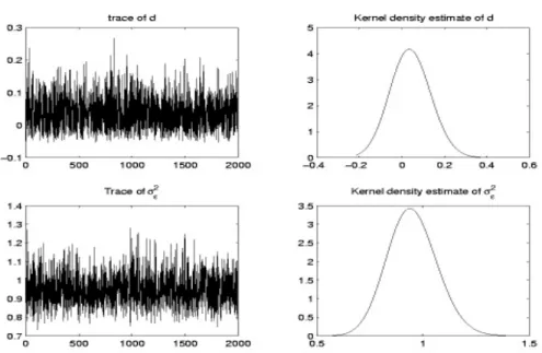
tenth one, after burn-in 500, with random initial values. The posterior inference is based on the actual random samples of 2000. For the case of

N=256, d=0.1,

σ

_ε2=1.0 and prior (b), Figure 1

shows the trace of the random samples and the kernel estimates of the posterior densities of the parameters.

The autocorrelation function of the random samples shows very little autocorrelations for the drawn series of the random samples. The two parallel chains mix well after small steps of the initial stage. All other diagnostics for convergence indicate a good convergence behavior.

In most cases, the Bayesian wavelet estimates of d and

σ

_ε2 are quite good. They are very close to the truth. The 95% credible interval

given by the Bayesian wavelet approach is well centered around the true parameter and is also very tight.

The estimation results using the two different priors (a) and (b) are very similar. The estimates by Jensen’s method differ most from those by the other methods. It seems that LA(8) generally gives better estimates than Haar. This is in agreement with the results of McCoy and Walden (1996) section 5.2.

Table 1: Estimation of the simulated I(d) process when N=256 Using Haar Basis. Prior (a) Prior (b)

Parameter Jensen MW Mean SD Mean SD

d=0.1 0.1620 0.1629 0.1686 0.0499 0.1692 0.0499 (0.0739, 0.2711) (0.0768, 0.2674) = 2 ε

σ

1.0 1.0226 1.0452 0.0931 1.0485 0.0977 (0.8801, 1.2460) (0.8791, 1.2540) d=0.25 0.1431 0.1858 0.1887 0.0465 0.1880 0.0462 (0.1049, 0.2827) 0.1008, 0.2854) = 2 ε

σ

1.0 1.0789 1.1000 0.0972 1.1068 0.1021 (0.9331, 1.3150) (0.9289, 1.3220) d=0.4 0.4121 0.4384 0.4301 0.0351 0.4284 0.0364 (0.3567, 0.4902) (0.3489, 0.4901) = 2 ε

σ

1.0 1.0189 1.0445 0.0934 1.0571 0.0975 (0.8775, 1.2395) (0.8822, 1.2640) d=0.1 0.1227 0.0681 0.0709 0.0470 0.0719 0.0472 (-0.0176, 0.1663) (-0.0172 0.1679) = 2 ε

σ

2.0 2.1482 2.1787 0.1918 2.1943 0.1948 (1.8455, 2.5745) (1.8570, 2.5975) d=0.25 0.2468 0.1855 0.1858 0.0477 0.1847 0.0462 (0.0995, 0.2858) (0.0938, 0.2785) = 2 ε

σ

2.0 1.9369 1.9674 0.1729 1.9791 0.1770 (1.6570, 2.3275) (1.6715, 2.3675) d=0.4 0.2154 0.3096 0.3127 0.0467 0.3105 0.0476 (0.2238, 0.4069) (0.2165, 0.4079) = 2 ε

σ

2.0 1.7783 1.8130 0.1540 1.8305 0.1619 (1.5435, 2.1385) (1.5300, 2.1665)

Table 2: Estimation of the simulated I(d) process when N=256 Using LA(8) Basis. Prior (a) Prior (b)

Parameter Jensen MW Mean SD Mean SD

d=0.1 0.0759 0.1701 0.1757 0.0466 0.1755 0.0446 (0.0894, 0.2734) (0.0936, 0.2707) = 2 ε

σ

1.0 1.0037 1.0222 0.0935 1.0270 0.0899 (0.8529, 1.2295) (0.8626, 1.2190) d=0.25 0.0904 0.2611 0.2651 0.0508 0.2661 0.0502 (0.1681, 0.3680) (0.1705, 0.3741) = 2 ε

σ

1.0 1.0154 1.0398 0.0916 1.0412 0.0888 (0.8791, 1.2295) (0.8824, 1.2255) d=0.4 0.4906 0.4369 0.4304 0.0359 0.4295 0.0362 (0.3548, 0.4905) (0.3536, 0.4895) = 2 ε

σ

1.0 1.0148 1.0413 0.0953 1.0502 0.0932 (0.8669, 1.2370) (0.8826, 1.2450) d=0.1 0.0542 0.1110 0.1175 0.0529 0.1151 0.0535 (0.0166, 0.2278) (0.0183, 0.2298) = 2 ε

σ

2.0 2.1233 2.1594 0.1926 2.1694 0.1894 (1.8185, 2.5765) (1.8235, 2.5650) d=0.25 0.1977 0.2609 0.2608 0.0535 0.2637 0.0540 (0.1556, 0.3697) (0.1630, 0.3761) = 2 ε

σ

2.0 1.8372 1.8745 0.1609 1.8849 0.1709 (1.5870, 2.2165) (1.5795, 2.2420) d=0.4 0.2632 0.3111 0.3130 0.0454 0.3117 0.0463 (0.2257, 0.4045) (0.2236, 0.4040) = 2 ε

σ

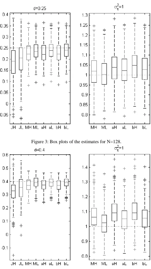
2.0 1.7469 1.7942 0.1635 1.7995 0.1595 (1.5080, 2.1510) (1.5145, 2.1225)

Figure 2: Box plots of the estimates for N=128.

Frequentist Comparison

Also compared were the estimates of the three methods in repeatedly simulated I(d) process. Figure 2 is the box plots of the estimates for d and

σ

_ε2respectively of 200 replicates with N=128, d=0.25 and

σ

_ε2=1.0. Figure 3 is the box plots of the estimates for 200 replicates with N=128, d=0.40 and

σ

_ε2=1.0. The x-axis labels in the box plot read as follows: `JH’ denotes the case by the Jensen method using Haar; ‘JL’ denotes the case by the Jensen method using LA(8); and so forth. Because of the long computation time associated with the Gibbs sampling for the large number of simulated I(d) processes, we limit the burn-in to 100 iterations and the number of random samples to 500. Because only the posterior mean was calculated using the generated random samples, not much information was lost even when the slightly short chain was used.

For the estimates of d, the mean square errors of the McCoy and Walden and The Bayesian method using these two priors are very similar, and they are all smaller than the one by Jensen’s OLS. LA(8) gives less biased estimates than Haar. The mean estimates for d given by the Bayesian method using LA(8) is similar to those by McCoy and Walden. In all methods, it seems the estimates for d and

σ

_ε2are a little biased in that

dˆ

tends to underestimate d and

2

ˆ_ε

σ

tends to overestimate

σ

_ε2. Conclusion

Bayesian wavelet estimation method for the stationary I(d) process provides an alternative to the existing frequentist wavelet estimation methods. Its effectiveness is demonstrated through Monte Carlo simulations implemented in the WinBUGS computing package.

A future effort is to extend the Bayesian wavelet method to more general fractional process such as ARFIMA(p,d,q). The hypothesis testing problem for the I(d) process can also be explored via the Bayesian wavelet approach.

References

Bardet, J., Lang, G., Philippe, A., Stoev, S., & Taqqu, M. (2003). Semi-parametric estimation of the long-range dependence parameter: a survey. Theory and Application of

Long-Range Dependence, Birkhauser.

Beran, J. (1994). Statistics for

long-memory processes. New York: Chapman and

Hall.

Daubechies, I. (1992). Ten lectures on

wavelets. SIAM

Davies, R. B., & Harte, D. S. (1987). Tests for Hurst effect. Biometrika,.74, 95-101.

Geweke, J., & Porter-Hudak, S. (1983). The estimation and application of long memory time series models. Journal of Time Series Analysis,

4, 221-238.

Granger, C. W. J., & Joyeux, R. (1980). An introduction to long-memory time series models and fractional differencing. Journal of

Time Series Analysis, 1, 15-29.

Hosking, J. R. M. (1981). Fractional differencing. Biometrika, 68, 165-176.

Jensen, M. J. (1999). Using wavelets to obtain a consistent ordinary least squares estimator of the long-memory parameter.

Journal of Forecasting, 18, 17-32.

Lunn, D., Thomas, A., Best, N., & Spiegelhalter, D. (2000) WinBUGS - A Bayesian modelling framework: Concepts, structure, and extensibility. Statistics and

Computing, 10, 325-337.

McCoy, E. J., Walden, A. T. (1996). Wavelet analysis and synthesis of stationary long-memory processes. Journal of

Computational & Graphical Statistics, 5, 26-56.

McLeod, B., & Hipel, K. (1978). Preservation of the rescaled adjusted range, I. A reassessment of the Hurst phenomenon. Water

Resources Research, 14, 491-518.

Vannucci, M., & Corradi, F. (1999). Modeling Dependence in the Wavelet Domain. In Bayesian Inference in Wavelet based Models. Lecture Notes in Statistics, Müller, P. and Vidakovic, B. (Eds). New York: Springer-Verlag.

Vidakovic, B. (1999). Statistical

modeling by wavelets. New York:

Wiley-Interscience.

WinBUGS 1.4: MRC, Biostatistics Group, Institute of Public Health, Cambridge University, Cambridge, 2003, www.mrc-bsu.cam.ac.uk/bugs

Appendix:

This appendix includes the MATLAB code for first simulating the I(d) process, then transforming it by DWT, and the WinBUGS program for the MCMC computation. In the WinBUGS programming, the symbol “~” is for the stochastic node which has the specified distribution denoted on the right side, the symbol “←” is for the deterministic node which has the specified expression denoted on the right side. All the likelihood function, the prior distributions

and initial values of the nodes without parents must be specified in the programs. The MATLAB code:

function x=Generatex(J, d, sig2eps) %Generate the I(d) process

%input:

%J: where N=2^J sample size

%d: long memory parameter of the I(d) process, abs(d)<0.5 %sig2eps: $\sigma_\epsilon^2$

%output:

%x: the time series N=2^J;

c=[];

% generate the autocovariance function by the formular of covariance % function for LRD

c(1)=sig2eps*gamma(1-2*d)/((gamma(1-d))^2);

%for i=1:N-1 c(i+1)=c(1)*gamma(i+d)*gamma(1-d)/(gamma(d)*gamma(i+1-d)); end; for i=1:N-1 c(i+1)=c(i)*(i+d-1)/(i-d); end;

x=GlrdDH(c);

function x=GlrdDH(c);

%GlrdDH.m Generating the stationary gaussion time seriess with specified % autocovariance series c

% using Davis and Harte’s method, Appendix of `Tests for Hurst Effect’, % Biometrika, V74, No. 1 (Mar., 1987), 95-101

%c: autocovariance series

[temp, N]=size(c); %c is a row vector cCirculant=[];

for i=1:N-2 cCirculant(i)=c(N-i); end; cFull=[];

g=[];

g=fft(cFull);

%Fast Fourier Transform of cFull Z=[];

Z=complex(normrnd(0,1,1,N), normrnd(0,1, 1,N));

Z(1)=normrnd(0,sqrt(2)); %Be careful to specify sqrt(2), if you want variance of Z(1) to be 2 Z(N)=normrnd(0,sqrt(2));

ZCirculant=[];

for i=1:N-2 ZCirculant(i)=conj(Z(N-i)); end; ZFull=[]; ZFull=[Z ZCirculant]; X=[]; X=ifft(ZFull.*sqrt(g))*sqrt(N-1); x=[]; x=real(X(1:N));

function [dJensen, dMW, sigMW, dBS, sigBS]=GetdHatSig2Hat(x, j0, filter) %Wavelet estimation of Long Range Dependence parameters

% %input:

%x: the observed I(d) process

%j0: lowest resolution level of the DWT %filter: wavelet filter

%output:

%dJensen: estimate of d by Jensen 1999

%dMW: estimate of d by McCoy & Walden 1996

%sigMW: estimate of $\sigma_\epsilon^2$ by McCoy & Walden 1996 %dBS: estimate of d by Bayesian Wavelet Method for prior (a), (b) %dBS.a, dBS.b

%sigBS: estimate of $\sigma_\epsilon^2$ by Bayesian Wavelet Method for prior (a), (b) %sigBS.a, sigBS.b

N=length(x); J=log2(N); w=[];

w = FWT_PO(x,j0,filter)’; %w is a coulmn vector resolution=[]; % data used in WinBUGS14 resolution(1:2^j0,1)=j0-1; for j = j0:(J-1) resolution(2^j+1 : 2^(j+1),1)=j; end; vwj=[]; for j=j0+1:(J-1) vwj(j, :)=[j, mean(w(dyad(j)).^2)];

end; tempd=[]; tempd=-[ones(J-2,1), log(2.^(2*vwj(2:J-1,1)))]\log(vwj(2:J-1,2)); dJensen=tempd(2); OPTIONS=optimset(@fminbnd); dMW=fminbnd(@NcllhMW, -0.5, 0.5, OPTIONS, j0, w, J); sigMW=findSig2epsHat(dMW, j0, w, J);

n=N-2^(J-1); %the first n data of w, approximation of variance %function mat2bugs() converts matlab variable to BUGS data file

mat2bugs(‘c:\WorkDir\LRD_data.txt’, ‘w’,w,’ twopowl’, 2^j0, ‘n’, n, ‘N’, N, ‘resolution’, resolution, ‘J’, J, ‘pi’, pi,’K’,500);

%set the current directory at MATLAB to ‘C:\Program Files\WinBUGS14\’ cd ‘C:\Program Files\WinBUGS14\’;

%prior (a)

dos(‘WinBUGS14 /par BWIdSt_a.odc’);

Sa=bugs2mat(‘C:\WorkDir\bugsIndex.txt’, ‘C:\WorkDir\bugs1.txt’); dBS.a=mean(Sa.d); %the posterior mean as the estimate of d

sigBS.a=mean(Sa.sig2eps); %the posterior mean as the estimate of sig2eps %prior (b)

dos(‘WinBUGS14 /par BWIdSt_b.odc’);

Sb=bugs2mat(‘C:\WorkDir\bugsIndex.txt’, ‘C:\WorkDir\bugs1.txt’); dBS.b=mean(Sb.d); %the posterior mean as the estimate of d

sigBS.b=mean(Sb.sig2eps); %the posterior mean as the estimate of sig2eps cd ‘C:\WorkDir’;

function y=NcllhMW(d, j0, w, J);

%NcllhMW.m --- Negative Concentrated log likelihood of McCoy & Walden %

%input:

%d: the long memory parameter, a value in (0,0.5) %j0: Lowest Resolution Level

%w: w=Wx, x is the observed time series %J: N=2^J sample size

% %output:

m=J-j;

bmP(j+1)=2*4^(-d)*quad(@sinf,2^(-m-1),2^(-m),[],[],d); %by McCoy & Walden’s formula, P37, (2.9)

smP(j+1)=2^m*bmP(j+1); end;

bpp1P=gamma(1-2*d)/((gamma(1-d))^2)-sum(bmP); %B_{p+1} in McCoy & Walden’s notation, p=J here spp1P=2^J*bpp1P*(bpp1P>0);

%S_{p+1} in McCoy & Walden’s notation, it should be nonnegative if spp1P>0 sig2epsHat=w(1)^2/spp1P; else sig2epsHat=0; end; sumlogsmP=0; for j = j0:(J-1) sig2epsHat=sig2epsHat+sum(w(2^j+1 : 2^(j+1)).^2)/smP(j+1); sumlogsmP=sumlogsmP+2^j*log(smP(j+1)); end; sig2epsHat=sig2epsHat/N;

%McCoy & Walden, Page 49, formular (5.1) y=N*log(sig2epsHat)+log(spp1P)+sumlogsmP; %McCoy & Walden, Page 49

function sig2epsHat=findSig2epsHat(d, j0, w, J);

%find Sig2epsHat by McCoy & Walden Page 49, formular (5.1) %

%input:

%d: the long memory parameter, a value calculated by function NcllhMW(); %j0: Lowest Resolution Level

%J: N=2^J sample size N=2^J;

bmP=[]; smP=[];

for j=j0:(J-1) %j is the resolution level m=J-j;

bmP(j+1)=2*4^(-d)*quad(@sinf,2^(-m-1),2^(-m),[],[],d); %by McCoy & Walden’s formula, P37, (2.9)

smP(j+1)=2^m*bmP(j+1); end;

bpp1P=gamma(1-2*d)/((gamma(1-d))^2)-sum(bmP); %B_{p+1} in McCoy & Walden’s notation, p=J here spp1P=2^J*bpp1P*(bpp1P>0);

N=2^J; bmP=[]; smP=[];

for j=j0:(J-1) %j is the resolution level if spp1P>0 sig2epsHat=w(1)^2/spp1P; else sig2epsHat=0; end; for j = j0:(J-1) sig2epsHat=sig2epsHat+sum(w(2^j+1 : 2^(j+1)).^2)/smP(j+1); end; sig2epsHat=sig2epsHat/N; \end{verbatim}

The WinBUGS script file: BWIdSt\_a.odc check(‘C:/MyDir/LRD_model_a.odc’) data(‘C:/MyDir/LRD_data.txt’) compile(1) gen.inits() update(100) set(d) set(sig2eps) update(500)

coda(*, ‘C:/Documents and Settings/MyDir/bugs’) #save(‘C:/Documents and Settings/MyDirlog.txt’) quit()

The WinBUGS model file: LRD_model_a.odc model {

# This takes care of the father wavelet coefficients from level L+1 to J-1 # which are detailed wavelet coefficients, $D$

for (i in twopowl+1:n) {

tau[i]<-1/(pow(2*pi, -2*d)*sig2eps*pow(2, 2*d*(J-resolution[i])) *(2-pow(2,2*d))/(1-2*d)) w[i] ~ dnorm (0, tau[i])

#The following takes care the wavelet coefficients at the resolution level J-1. #It uses the exact formula instead of the approximation.

for (i in 1:K) { sinf[i]<-pow(sin(pi*(0.25+i/(4*K))),-2*d)} integration<-sum(sinf[])/(4*K)

B1<-2*pow(4,-d)*sig2eps*integration

tau1<-1/(2*B1) #S_1=2*B_1 in McCoy & Walden 1996’s notation

for (i in (n+1): N) { w[i] ~ dnorm (0, tau1) }

# This takes care of the scaling coefficients on the lowest level $j_0=L$ # which are mother wavlelet coefficients, $C$

# twopowl <- pow(2, L)

for (jp1 in 1:J-1) { #jp1=j+1, m=J-j

b[jp1]<-(2*pow(2*pi, -2*d)*sig2eps*pow(2, -(J-jp1+1)*(1-2*d)) *(1-pow(2,2*d-1))/(1-2*d)) }

bpp1<-sig2eps*exp(loggam(1-2*d))/pow(exp(loggam(1-d)),2)-sum(b[])-B1; #B_{p+1} in McCoy & Walden’s notation

spp1<-pow(2,J)*bpp1*step(bpp1)+1.0E-6;

#S_{p+1} in McCoy & Walden’s notation, this should be positive tau0 <- 1/spp1

for (i in 1: twopowl) { w[i] ~ dnorm(0, tau0) }

#note: m=J-resolution[i] in McCoy & Walden’s 1996 paper # prior (a) d~dunif(-0.5, 0.5) sig2eps<-1/ tau2 tau2~dgamma(1.0E-2,1.0E-2) #prior (b) # d~dunif(-0.5, 0.5) # sig2eps~dunif(0,1000) }