Between Restarts and Backjumps
Antonio Ramos, Peter van der Tak, and Marijn Heule⋆
Department of Software Technology, Delft University of Technology, The Netherlands
Abstract. This paper introduces a novel technique that significantly reduces the computational costs to perform a restart in conflict-driven clause learning (CDCL) solvers. Our technique exploits the observation that CDCL solvers make many redundant propagations after a restart. It efficiently predicts which decisions will be made after a restart. This prediction is used to backtrack to the first level at which heuristics may select a new decision rather than performing a complete restart. In general, the number of conflicts that are encountered while solving a problem can be reduced by increasing the restart frequency, even though the solving time may increase. Our technique counters the latter effect. As a consequence CDCL solvers will favor more frequent restarts.
1
Introduction
Restarts are used in satisfiability (SAT) solvers to avoid heavy-tail behavior [4]. Restart strategies [7,14] have been a crucial feature in conflict-driven clause learning (CDCL) solvers [8] to tackle hard industrial problems. These solvers favor frequent restarts in recent years [5].
CDCL solvers select decision variables based on their involvement in emerged conflicts [10]. In case of frequent restarts, only several new conflicts have been hit between two succeeding restarts. As a consequence, CDCL solvers tend to select the same variables in a similar order after succeeding restarts. Additionally, phase-saving [12] ensures that decision variables are assigned to the same truth value as the value they were assigned to before a restart. Due to these heuristics, CDCL solvers generally do not perform a full restart, but effectively they perform
a partial restart.
This paper capitalizes on this observation by introducing two techniques to reduce the computational costs to perform a restart. In case the solver wants to restart, we show how to efficiently predict the first level at which the heuristics may select a different decision variable. The solver can perform a partial restart by backtracking to this level, rather than perform a more costly full restart.
Additionally, by reducing the restart costs, it appears that restarting even more frequently improves the performance of CDCL solvers. We implemented our techniques inMiniSAT2.2 [2]. Experiments show that the enhanced version with rapid restarts solves more real-world SAT instances from the SAT 2009 application suite than the original version.
⋆
The remainder of this paper is structured as follows: the next section pro-vides some background information about CDCL solvers and corresponding ter-minology. In Section 3 we motivate our work and Section 4 presents two novel techniques to reduce the computational costs to perform a restart. Experimental results are described in Section 5. Finally, we offer suggestions for future work in Section 6 and we draw conclusions in Section 7.
2
Conflict-Driven Clause Learning Solvers
The strategy used by conflict-driven clause learning (CDCL) solvers is to make a series of decisions (heuristically chosen assignments) and to propagate assign-ments that can be derived from these decisions by means of unit propagation (satisfying the remaining literal in every unit clause). The solver will continue to make decisions and propagate information until either a satisfying assignment is found for the problem, or a conflict emerges.
A conflict emerges if the solver finds aconflicting clause – a clause for which all literals are false. When this occurs, the solver analyzes the reason for the conflict. This is captured in a so-calledlearned clause [9,10] , which intuitively can be considered a clause that will avoid recurrence of the same combination of assignments that led to the conflict. Now, the solver unassigns variables until the learned clause becomes unit and continues to make decisions and apply other unit propagations as before.
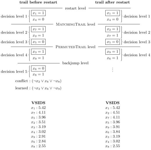
The terminology introduced in this section is used in the remainder of this paper. Fig. 1 graphically shows the most important terms. This figure will also be used as a running example throughout the paper.
2.1 Heuristics
In addition to the general process described above, most CDCL solvers use the Variable State Independent Decaying Sum (VSIDS) heuristic [10] to determine the order in which decisions should be made. This heuristic stores an activity value for each variable, which is increased by 1 whenever a variable appears in a learned clause. After incrementing the activity value, the value of every variable is decreased by multiplying them with a constant factor δ1, called the variable decay. This decay factor δ has a value in interval (0,1). In general, CDCL solvers useδ= 0.95. The lower the value ofδ, the more VSIDS prefers to select variables that were involved in recent conflicts. When no more information can be propagated, a new decision is made by selecting the unassigned variable with the highest activity value.
After a decision variable is selected by the solver, it must be assigned a value. A commonly used method is phase-saving [12], which stores for each variable the last value to which it was assigned by unit propagation. Decision variables are assigned to that value. By assigning variables to their last implied value, the
1
In practice, VSIDS is implemented by multiplying the incremental value by1
solver picks up where it left off and continues its search in a similar part of the search space after a restart. Therefore, phase-saving facilitates frequent restarts.
2.2 Decision levels and Backjumping
Each decision introduces a new decision level. A decision level consists of the sequence of assignments of a decision variable and all variables that are implied by that decision. Decision levels are numbered incrementally, where 0 is the level where no decisions have yet been made – also known as therestart level. Decision level 1 is the first level that involves an actual decision. A decision is the first assignment in each level (denoted in Fig. 1 by the rectangles), other assignments, if any, are caused by unit propagation.
The decision levels form a trail of assignments. This trail can be seen as a list of variable assignments at a certain moment in time. The trail comprises both decisions and unit propagations, where each decision starts a new decision level. Finally, thebackjump level [3] is the level to which the solver backtracks whenever a conflict is found. This is the level at which the learned clause is a unit clause. Notice that backjumping could be seen as performing a partial restart.
2.3 Restart Strategies
Modern solvers use restarts to avoid spending too much time searching for a solution in the same region without finding useful information. By restarting, CDCL solvers try to avoid heavy-tail behavior [4]. When a restart is performed, the solver will undo every assignment on the trail and make a new series of decisions and propagations. Because the learned clauses and the VSIDS heuristic will have changed since the previous run, the new run may perform decisions in a different order. This could reduce the total number of decisions necessary to solve a problem [6].
A commonly used restart strategy in recent years is based on a sequence of restart sizes suggested by Luby et al. [7]. In their work the authors show that the suggested sequence is log optimal when the runtime distribution of the problems is unknown. In this strategy the length of restartiisu·ti whenuis a constant
unit run and
ti= ( 2k−1 , ifi= 2k −1 ti −2 k−1+1, if 2k−1≤i <2k−1.
Since unit runs are commonly short, solvers using the Luby restart strategy exhibit frequent restarts. The solvers Rsat[12] and TiniSat[6] use a unit run of 512 conflicts, while MiniSAT 2.2 [2] andprecoSAT[1] use a shorter unit run of 100 conflicts.
In this paper, we proposepartialrestarts which can be combined with these
fullrestart strategies. An alternative partial restart strategy that has been pro-posed israndom jump[15]. This strategy randomly backtracks to a level between the restart level and the backjump level. In [11] a technique is proposed to par-tially restart based on the learned clause if certain conditions are met.
F = (¬x1∨x2∨ ¬x7)∧(¬x1∨ ¬x4)∧(x1∨x5)∧(¬x2∨x6∨ ¬x8) ∧ (¬x2∨x4∨x7)∧(x3∨ ¬x5∨ ¬x6)∧(¬x3∨x9)∧(x6∨x8∨ ¬x9)
trail before restart trail after restart restart level x1= 1 x1= 1 x4= 0 x4= 0 MatchingTraillevel x7= 1 x2= 1 x2= 1 x7= 1 x5= 0 x5= 0 PermutedTraillevel x3= 1 x9= 1 x9= 1 x6= 1 backjump level x6= 0 .. . x8= 1 conflict : (¬x2∨x6∨ ¬x8) learned : (¬x2∨x6∨ ¬x9) VSIDS x1: 5.42 x7: 4.11 x5: 3.96 x2: 3.51 x3: 3.19 x4: 3.02 x9: 2.91 x6: 2.84 x8: 2.55 VSIDS x1: 5.42 x2: 4.51 x7: 4.11 x5: 3.96 x9: 3.91 x6: 3.84 x3: 3.19 x4: 3.02 x8: 2.55 decision level 1 decision level 2 decision level 3 decision level 4 decision level 5 decision level 1 decision level 2 decision level 3 decision level 4
Fig. 1.Visualization of our running example. Example of the outcome of Matching-Trail and PermutedTrail. In both trails, the first five assigned variables are x1, x2,x4,x5, and x7, albeit in different order. Therefore, backtracking to decision level 3 – right after the five matching assignments – causes the state of the solver to be equivalent to the state after restarting to decision level 0 and assigning the first five variables.
3
Motivation
The main contributions of this paper are two techniques to reduce the compu-tational costs of performing a restart. In this section, we motive our work. First, we argue that CDCL solvers actually perform a partial restart and we indicate how to capitalize on that observation (Section 3.1). Second, we show that CDCL solvers traverse a smaller part of the search space when they restart more fre-quently. However, due to the restart costs, this may not always translate into improved performance (Section 3.2).
3.1 Partial Restart
The first observation that inspired the work below is that modern CDCL solvers usually make partial restarts rather than a full one. Yet in practice a full restart is performed, followed by the setup of a similar trail to the one that was just removed. By avoiding the redundant propagations, the cost of a restart can be reduced significantly.
Consider our example formulaF and the two trails shown in Fig. 1. At the bottom of this figure the activities (VSIDS scores) are shown. Due to the learned clause (¬x2∨x6∨ ¬x9) the activity of the corresponding variables is increased by 1, which slightly changes the order. Recall that the variable with the highest activity that is not yet assigned is always selected as the next decision. The left part of Fig. 1 shows the assignments before the restart; the right shows the assignments after.
Let us compare the two trails. The first similarity is that decision level 1 is exactly the same before and after the restart, because variablex1 still has the highest VSIDS score after the restart. Due to this similarity, the solver actually performs a partial restart. Yet this observation is not exploited by current solvers. As a result, they perform redundant propagations. Because the second decision after the restart isx2 (instead ofx7), the trails no longer match. We denote by MatchingTrail, the last level at which the trails before and after a restart completely match. We show how to compute this level efficiently in Section 4.1. A second similarity can be observed between the two trails. Notice that (i) the first five variables in both trails are the same and (ii) that these variables are assigned to the same values in the new trail as in the former trail. This is not a coincidence. The reason for (i) is that CDCL solvers restart frequently. Therefore, only a few clauses are learned between two restarts. This changes the VSIDS order of the variables only slightly. Additionally, (ii) is ensured by the phase-saving heuristic which is used by most CDCL solvers.
Since we know that there are no new propagations before the backjump level, the only difference in the trail is that the order of variables are permuted. We denote the last level at which both (i) and (ii) hold by PermutedTrail. Notice that at the PermutedTrail level the reduced formula is exactly the same before and after the restart. Therefore, performing a partial restart to the PermutedTraillevel is similar to performing a full restart. Section 4.2 shows how to compute this level efficiently.
3.2 Restart Frequency
Another observation regarding restarts in modern CDCL solvers was presented in [5] showing that restarting with shorter unit runs reduces the size of the search space the solver explores to tackle a problem. More specifically, more frequent restarts reduce the number of conflicts encountered during the search.
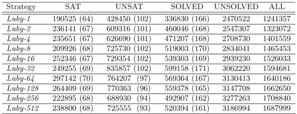
We computed the effect of Luby-based restarts with various unit runs on the average number of conflicts. The only difference between our experiment and [5] is the use of the latest version ofMiniSAT(2.2) [2]. The results for the SAT 2009 application suite are shown in Table 1.
Table 1.Average number of conflicts for several unit runs of the Luby sequence. The numbers between brackets denote the number of solved instances within 1200 seconds. We used three seeds to initialize the VSIDS scores to obtain a more stable image.
Strategy SAT UNSAT SOLVED UNSOLVED ALL Luby-1 190525 (64) 428450 (102) 336830 (166) 2470522 1241357 Luby-2 236141 (67) 609316 (101) 460046 (168) 2547307 1323072 Luby-4 235651 (67) 626690 (101) 471207 (168) 2708730 1401559 Luby-8 209926 (68) 725730 (102) 519003 (170) 2834041 1465453 Luby-16 252346 (67) 729354 (102) 539303 (169) 2939230 1526033 Luby-32 249255 (69) 835857 (102) 599158 (171) 3062220 1594681 Luby-64 297142 (70) 764207 (97) 569364 (167) 3130413 1640186 Luby-128 264409 (69) 770363 (96) 559378 (165) 3147708 1662650 Luby-256 222895 (68) 688930 (94) 492907 (162) 3277263 1708840 Luby-512 238800 (68) 725555 (93) 520394 (161) 3186994 1687999
First consider the number of solved instances shown in the first three columns. Although the Luby unit run is incrementally increased by a factor two, the number of instances solved remains quite comparable. The biggest differences are on the satisfiable instances. This was expected because CDCL solvers are not very stable on those formulas. When comparing the average number of conflicts, we observe that the longer the unit run, the higher this average. For the longest unit runs, we do not observe this pattern. These averages have been influenced by the lack of solved hard unsatisfiable instances within the timeout.
The last two columns show a clearer pattern regarding the average number of conflicts. Both columns are almost strictly increasing. Based on the data in these columns we can estimate the number of conflicts per second for different unit runs. Both the averages shown in the UNSOLVED and ALL columns indicate that the long unit runs handle about 35% more conflicts per second compared to the short unit runs. This difference is likely to be caused by restart costs.
By restarting with a short unit run, the solver encounters on average fewer conflicts while solving a problem. However, due to the costs of restarting fre-quently, using shorter unit runs does not result in solving more instances. In fact, both effects appear to cancel each other out since the various settings solve practically the same number of instances. We aim to reduce the costs of restarts which should in turn favor solvers that restart more frequently.
4
Reducing Restart Costs
This section describes the two algorithms we propose to compute the level to which to backtrack, MatchingTrail and PermutedTrail. The algorithms rely on phase-saving, VSIDS ordering, and the absence of random decisions – all default in e.g. the latestMiniSAT2.2. Furthermore, they should have access to the assignment type of each variable (Decision, Implication, Unassigned) and the decision level at which the variable was assigned. In the algorithms these are denoted by AssignmentT ype[x] andDecisionLevel[x] respectively, wherex is a variable.
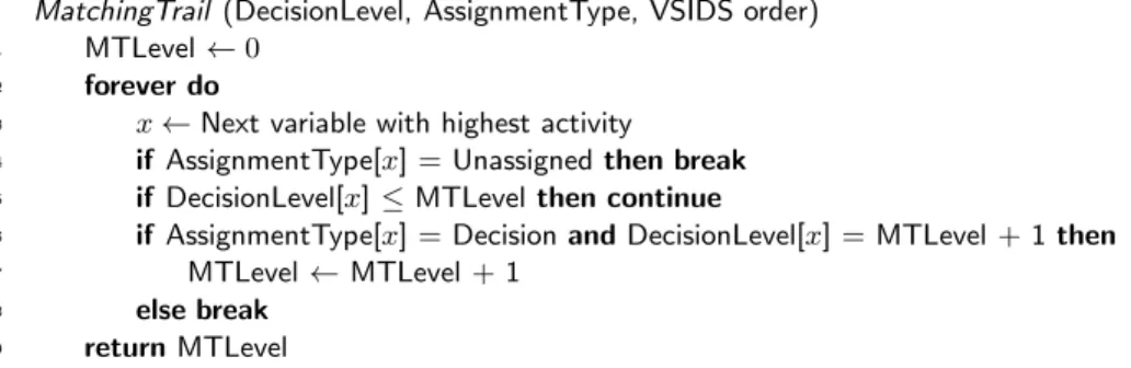
4.1 Matching Trail
Fig. 2 shows the pseudo-code of how to compute the MatchingTrail level. The algorithm increases M T Levelfor every decision that will be made at the same level in the current trail and the trail after the restart. The algorithm loops through variables in descending order of activity. If the variable is not currently assigned, the next decision level after the restart will be different and the algorithm will terminate (Line 4). If the variable is already assigned a value
at M T Levelor before, it will be an implied variable in both trails and can be
ignored (Line 5). Finally, if it is a decision variable, it will be the next decision in the trail after the restart. Therefore, if the variable matches the decision at
M T Level, a match is found and M T Levelis incremented (Line 7). If not, the
decisions at the next level will be different, and the algorithm returns the last level at which they were the same (Line 9).
Example. Again consider the example in Fig. 1. The algorithm starts with
M T Level= 0 and considersx1. It detects that both trails will have matching
decisions at level 1, and increments M T Levelto 1. Next, variable x2 is found to become the decision at level 2 after the restart, but it does not match deci-sion variable x7 at the same level of the current trail. Therefore, the algorithm terminates and returnsM T Level= 1.
MatchingTrail (DecisionLevel, AssignmentType, VSIDS order)
1 MTLevel←0
2 forever do
3 x←Next variable with highest activity
4 if AssignmentType[x] = Unassignedthen break 5 if DecisionLevel[x]≤MTLevelthen continue
6 if AssignmentType[x] = DecisionandDecisionLevel[x] = MTLevel + 1then
7 MTLevel←MTLevel + 1
8 else break
9 returnMTLevel
Fig. 2.Pseudo-code of theMatchingTrailalgorithm. This algorithm returns the last level at which all decisions will occur in the exact same order after the restart.
4.2 Permuted Trail
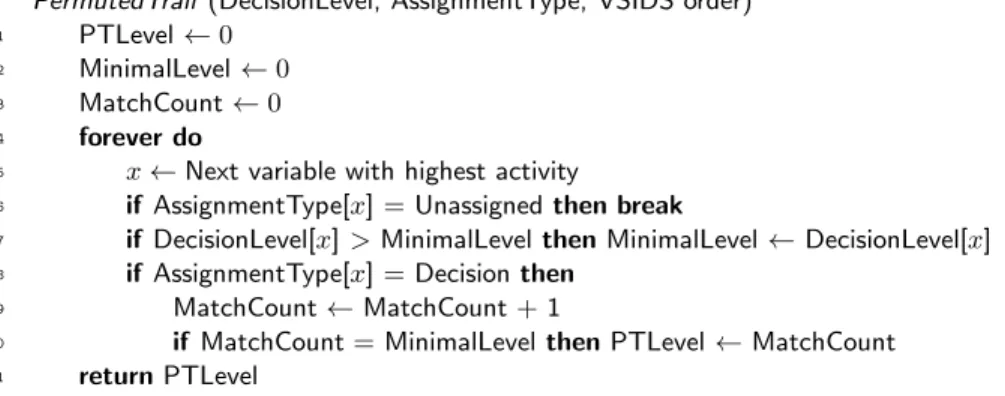
ThePermutedTrailalgorithm (Fig. 3) aims to compute the last level at which the partial assignment (and hence the reduced formula under this assignment) is exactly the same before and after a restart (recall Section 3.1). Like Matching-Trail,PermutedTrailloops through variables in descending order of activity. For each variable, it determines at which level it was assigned, and stores the running maximum inM inimalLevel(Line 7). This value represents the level at which all variables that have been processed so far have been assigned. Also, it counts how many of these are currently decision variables, and stores this value
in M atchCount(Line 9). Any variable that is currently unassigned terminates
the algorithm, since this variable will become a decision that can never be part of a permutation of the current trail (Line 6).
Now consider what happens whenM atchCount=M inimalLevel. By defi-nition ofM inimalLevel, the set of variables that the algorithm has processed so far is a subset of the variables that are assigned up to M inimalLevel. Because this set includes M atchCountdecision variables, it must include each decision variable up to M inimalLevel. Since at least the same decisions are made, unit propagation will ensure that any currently implied variable is also assigned after the restart. Since the algorithm is performed at the backtrack level, no addi-tional unit clauses may appear in the trail after the restart up to this point, which means that both trails must contain the exact same variables. Therefore the algorithm indicates that a partial restart is possible at this level inP T Level
(Line 10).
PermutedTrail (DecisionLevel, AssignmentType, VSIDS order)
1 PTLevel←0 2 MinimalLevel←0 3 MatchCount←0
4 forever do
5 x←Next variable with highest activity
6 if AssignmentType[x] = Unassignedthen break
7 if DecisionLevel[x]>MinimalLevelthenMinimalLevel←DecisionLevel[x] 8 if AssignmentType[x] = Decisionthen
9 MatchCount←MatchCount + 1
10 if MatchCount = MinimalLevelthenPTLevel←MatchCount
11 return PTLevel
Fig. 3. Pseudo-code of the PermutedTrail algorithm. This algorithm returns the
decision level at which all decisions occur in the trail after the restart (so that there are no intermediate decisions), but possibly in a different order.
Example. Consider how the algorithm will find thePermutedTrail level for the running example in Fig. 1. The algorithm starts considering x1, which is set in decision level 1, so that M inimalLevel is set to 1. Since it is also a decision variable, M atchCount is incremented to 1. The values match, and hence the algorithm finds that a partial restart is possible at P T Level = 1. Next,x2 has the highest activity. It is a propagation in level 2, and it updates
M inimalLevel= 2 and M atchCount= 1. Next,x7 is a decision in level 2, so
thatM inimalLevel=M atchCount= 2. Both values match, andP T Level= 2
is another possible backtrack level for a partial restart. Note that this is detected even thoughx2 became a decision variable andx7 became an implied variable. Now x5 is considered, leading to M atchCount = M inimalLevel = 3, which means thatP T Level= 3 is the best candidate so far. Forx9,M inimalLevel= 4
and M atchCount= 3, so thatP T Level= 3 remains unchanged. Finally,x6 is
currently unassigned because the algorithm runs after backtracking to the back-jump level. The algorithm thus terminates withP T Level= 3.
4.3 Discussion
The MatchingTrail technique has the nice feature that solvers will explore the search space exactly the same as when performing a full restart. Yet al-though the reduced formula before and after a restart is exactly the same at the PermutedTraillevel, the solver may explore the search space differently when this technique is applied. This is caused by the so-calledreason clauses[2]. The reason clause for an implied variable is the one that assigned its truth value (the first to become unit). Reason clauses are used to compute learned clauses. By making decisions in a different order, the reason clauses may be different, which in turn could make the conflict clauses different. This may influence the way the search space is explored.
Ideally one wants to backtrack to the last level at which the partial assign-ment is exactly the same before and after a restart. Although the Permuted-Trailalgorithm is designed to do that, it may return a “subprime” level.
To illustrate this, let LastSameAssignment be the ideal backtrack level (i.e. the last level where the partial assignment is the same before and after the restart). Letybe the decision variable at theLastSameAssignmentlevel. Now, assume that there is a variable xwhich is a decision variable before the LastSameAssignmentlevel in the current trail, and which has a lower activity thanyafter the restart. Because the partial assignment is the same,xis assigned in the trail after the restart, and because it has a lower activity thanyit must be an implied variable. However, using thePermutedTrailalgorithm, we cannot detect thatxis implied by the assignments in the new trail. Therefore it will not return the LastSameAssignment level. During our experiments we observed that in practice this does not occur often, so that there is not much difference be-tween the level returned byPermutedTrailand theLastSameAssignment level.
5
Experimental Results
We implemented MatchingTrail and PermutedTrail in MiniSAT 2.2 and configured it to facilitate our analysis. There are three main requirements for us-ing the proposed algorithms: phase-savus-ing, the VSIDS heuristic, and the absence of random selection of decision variables. Each of these is default inMiniSAT2.2, therefore the implementation of the algorithms was easy and straightforward.
We used the (292) application instances of the SAT 2009 competition2 . Each instance was run with a time limit of 1200 seconds using different configurations on a server of 20 Intel Xeon X5570 CPUs running on 2.9 GHz with 32 GB of memory.
5.1 Matching Trail
It turned out that theMatchingTrailalgorithm was much less effective than the PermutatedTrail algorithm. Fig. 4 shows a typical distribution of the MatchingTrail,PermutedTrail, and backjump levels. The distributions of the PermutedTrail and backjump level are quite comparable. However, the MatchingTraillevels are generally much lower – which explains why it is less successful in reducing the restart costs. Therefore, we focused our experiments on the usefulness of thePermutedTrailalgorithm.
decision level fr eq u en cy 1 10 100 1000 10000 0 50 100 150 200 backjump level PermutedTraillevel MatchingTraillevel
Fig. 4.Distribution of theMatchingTrail,PermutedTrail, and backjump levels
while solving the ACG-15-10p1.cnf benchmark of the SAT 2009 competition using MiniSAT2.2 with a Luby-1 restart strategy.
2
5.2 Permuted Trail
In this section we compare the performance of MiniSAT 2.2 with and without PermutedTrail. Comparing the performance of SAT solvers is hard, because a small change, for example to the order in which unit propagation is applied, can have a huge impact on the performance. Therefore, our focus in this section is not only on solving time, but also on the number of conflicts per second. The latter seems a bit more robust (recall also Section 3.2).
We experimented with three restart strategies. First, the default strategy of
MiniSAT 2.2, which uses the Luby sequence with a unit run of 100 (in short
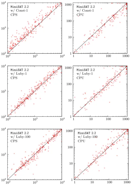
Luby-100). Second, because we expect that the PermutedTrail technique is especially useful for short unit runs, we added the strategy with the shortest unit run 1 (Luby-1). Third, we included a radical strategy that restarts before ev-ery decision (Const-1). This strategy would profit most fromPermutedTrail, showing thereby the maximum one could gain using this technique. Notice that a CDCL solver with the Const-1 restart strategy is still complete [13].
Fig. 5 shows the number of conflicts per second (left) and the solving time (right) forMiniSAT using the three restart strategies with and without partial restarts to the PermutedTrail level. The Const-1 and Luby-1 strategies can clearly process more conflicts per second when PermutedTrail is enabled. For the Luby-100 strategy no real improvement is observable, as expected. For some instances, the PermutedTrail actually had a negative effect. For these benchmarks the performance greatly depends on the seed3.
In our last experiment, we wanted to see whether the use of Permuted-Trailwould make a rapid restart strategy preferred over the default Luby-100. In the tests above we used the default variable decay ofMiniSATδ= 0.95 (see Section 2.1). However, preliminary tests showed that when using rapid restarts such as Const-1 and Luby-1, a lower value of the δ results in improved per-formance. Notice that a lower variable decay will makePermutedTrail itself a bit less effective because variables will go up and down faster in the VSIDS order. We found thatδ= 0.75 results in strong performance. Therefore, in this last experiment we combined PermutedTrail with δ = 0.75 (denoted by an asterisk, e.g. Luby-1*).
Figure 6 shows the results. CombiningPermutedTrail with δ= 0.75 in-creases the number of instances solved for each restart strategy, especially for Const-1 (156 vs 168 instances solved) and Luby-1 (173 vs 187 instances solved). The impact on Luby-100 is hardly visible. This is expected since this strategy restarts much less frequently, therefore the cost reduction of restarts hardly in-fluences the performance. Luby-1* performed best during our experiments. This shows that PermutedTrail reduced the restart costs to such level that the benefits of encountering fewer conflicts to solve a problem can be exploited to the point where it solves 10 instances more than the default configuration of
MiniSAT.
3
MiniSAT has the option to randomly initialize the VSIDS scores. For many bench-marks the seed used for the initialization has a huge impact on the performance.
MiniSAT2.2 w/Const-1 CPS 102 103 104 102 103 104 + + + + + + + + + + + + + + + + + + + + + + + + + + + + + + + + + + + + + + + + + + + + + + + + + + + + + ++ + + + + + + + + ++ + + + + ++ + + + + + +++++ + ++ + + + + + + + + + + + + + + + + + + + + + + + + + + + + + + + + + + + + + + + + + + + ++ + + + ++ + + + + + ++ + + + + + + + + + + + + + + ++ + ++ + + + + + + + + + + + + + + + + + + + ++ + + + + + + + + + + + + + ++ + + + + + + + + + + + + + + + + + + + + + + + + + + + + + + + + ++ + + + + + + + + + + + + + + + + + MiniSAT2.2 w/Const-1 CPU 1 10 100 1000 1 10 100 1000 +++++++++ + + + ++++++ + + + +++ + + + + + + + + + + + + + + + +++ + ++ + ++ + ++++ + + + + + ++++++ + + + + + + + + + + + + + + +++++++++++ + + + + + + ++++ + + ++ + ++ ++ + + + + + + + + + + +++ + + + + + + + + + +++++++++++++++++++ + ++ +++++ + +++++ + ++ + + + + + + + + + + + + + + + + + + + ++ ++++ + + + ++++++ + + +++++++ + ++ + + + + + + + + + ++++ + ++ + ++ + + + + + + + + + + + + + + ++ ++++ + + ++ + + + + + + + + + + + + + + + + + + + + + + ++ MiniSAT2.2 w/Luby-1 CPS 102 103 104 102 103 104 + + + + + + + + + + + + + + + + + + + + + + + + + + + + + + + + + + + + + + + + + + + + + + + + + + ++ + + + + + + + + + + + + + + + + + + + ++ + ++ + ++ + + ++++ + + + + + + + + + + + + + + + + + + + + + + + + + + + + + + + + + + + + + + + + + + + + + + + + + + + + + + + +++ + + + + + ++ + + + + + + + + + + + + + + + ++ + + + + + + + + + + + + + + + + + + + + + + + + + + + + + + + + + + ++ + + + + + + + + + + + ++ + + + + + + + ++ ++ + + + + + + + + + + + + ++ + + + + + + + + + + + ++ MiniSAT2.2 w/Luby-1 CPU 1 10 100 1000 1 10 100 1000 + ++++++++ + + + + +++++ + + + +++ + + + + + + + + + + + + + + + +++ + ++ + ++ + + + ++ + + + + ++++ + + + + + + + + + + + + + + + + +++++++++++ + + + + + + ++++ + + ++ + ++ + + + + ++ + + + + + + +++ + + + + + + + + + + + + + + + +++++++++++++ +++ +++++ + + + +++ + + + + + + + + + + + + + + + + + + + + + + + + + + + + + + + ++++++ + + +++++++ + ++ + + + + + + + + + ++++ + ++ + + + + + + + + ++ + + + + + + + + + ++++ + + ++ + + + + + + + + + + + + + + ++ + + + + + +++ MiniSAT2.2 w/Luby-100 CPS 102 103 104 102 103 104 + + + + + + + + + + + + + + + + + + + + + + + + ++ + + + + + + ++ + + + + + + + + + + + + + + + + + + + + + + + + + + + + + + + + + + + + + ++ + + + +++++ + + ++ + ++++ + + + + + + + + + + + + + + + + + + + + + + + + + + + + + + + + + + + + + + + + + + + + + + +++ + + + + + + + + ++ + + + + + + + + + + + + + + ++++ + + + + + + + + + + + + + + + + + + + + + + + + + + + ++ + ++ + + + + + + + + + + + + + + + + + + + + + + + + + + + + + ++ + + + + + + + + + + + + + + + + + + + MiniSAT2.2 w/Luby-100 CPU 1 10 100 1000 1 10 100 1000 +++++++++ + + + ++++ +++ + + +++ + + + + + + + + + + + + + + +++ + ++ + ++ + + +++ + + + + ++++ + + + ++ + + + + + + + + + +++++ + +++++++ + + + + + + ++++ + + + + + + + + + + + + + + + + + + +++ + + + + + + + + + + + + + + + + + +++++++++++ ++ + ++ + ++ + + + + + + + + + + + ++ + + + + + + + + + + + + + + + + + + ++ + + ++++++ + + +++++++ + ++ + + + + + + + + + ++++ + ++ + + + + + + + + + + + ++ + + + + + + +++ + + + ++ + + + + + + + + + + + + + +++ + + + + + + + +
Fig. 5. Comparison of the number of conflicts per second (left) and solver runtime (right) between full restarts andPermutedTrailfor the SAT 2009 application
bench-marks.PermutedTrailpropagates more conflicts per second above the diagonal (left) and solves instances faster below the diagonal (right).
0 200 400 600 800 1000 1200 0 50 100 150 200 ti m e (s )
number of instances solved Const-1 ++++++++++++++++++++++++++++++++++++++++++++++++++++++++++++ ++++++++++++++++++ ++++++++++++++++ ++++++++ ++++++++ ++++++++ ++++ +++++ +++ ++ + + ++ + +++ ++++ + ++ ++ + +++ ++ + + Const-1* r r r r r r r r r r r r r r r r r r r r r r r r r r r r r r r rr r r r r r r r r r r r r r r rr r r r r r r r r r r r r r r rr r r r r r r r rr r r r r r r r rr r r r r r r r rr r r r r rr r rr r r r r rr r rr r r r r rr r r rr rr r r r r r r r rr r r rrr r rrr r r r rr r r r rr r rr r r rr r r r r r r r r r r r r Luby-1 b b b b b b b b b b b b b b b b b b b b b b b b b b b b b b b b b b b b b b b b b b bb b b b b b b b b b b b b b b b b b b bb b b b b b b bb b b b b b bb b b b b b bb b b b bb b b b b b b b b bb b b bb b b b b b b bb b b bb b b b b b b b bbb b b bb b b bb b b b b b bb bb bb b b bb bb bb bb b b b b b bb b bb b bb b b b b b Luby-1* +++++++++++++++++++++++++++++++++++++++++++++++++++++++++++++++++++++ ++++++++++++++++++++ +++++++++++++++++++ +++++++++ +++++++++++ ++++ ++++ +++ ++++++++ ++ ++ ++ +++++ +++++ +++ ++++ ++ +++ + + ++ ++ +++ +++ + Luby-100 u u u u u u u u u u u u u u u u u u u u u u u u u u u u u u u u u u u u u u u u u u u u u u u uu u u u u u u u u u u u u u u u u u u uu u u u u u u u u u uu u u u u u uu u u uu u u u u u u u u u u u u uu u uu u u uuu u u u uu uu u u u u u uu u u u uuu u uu uu u u uu uu u uuu uu u u u u u u uu u u u u u uu uu u u u uu u u uu u u Luby-100* r r r r r r r r r r r r r r r r r r r r r r r r r r r r r r r r r r r r r r r r r rr r r r r r r r r r r r r r r r r rr r r r r r r r r r r r r r rr r r r r rr r r r r r r rr rr r r r r r r r r r rr r r r rr r r rrr r r rr r rr r r r r rrr r r r rr r r rr rr rr r rr r r r rr r r r r r rr r rr r r r r rr r r r r rr rr r r rr rr r r r
Fig. 6.Cactus plot showing the number of instances solved versus the time required to do so for three restart strategies and two configurations. PermutedTrail with
δ = 0.75 – denoted in the legend with an asterisk – improves the performance of MiniSAT.
6
Suggestions for Future Work
Although our algorithm finds a reasonably high partial restart level, the solver still performs redundant work sometimes when a decision variable becomes an implied variable after a restart (recall Section 4.3). The current algorithms will not always detect that, and therefore may not return the optimal backtrack level. Although we have not seen this happen frequently in practice, it is possible that for some instances this occurs often, in which case it might be interesting to further analyze this issue and to develop efficient solutions.
We expect that the performance improvements are mainly caused by the reduced restart costs. Yet, the PermutedTrail algorithm has also an impor-tant side effect. After a full restart, the reason clauses of implied variables may change, while after a partial restart the reason clauses stay the same. We want to study whether this effect influences the performance positively or negatively.
7
Conclusion
In this work, we implemented and tested two performance enhancements that reduce restart costs for CDCL solvers. We implemented both techniques in the latest MiniSAT solver. We show how to reduce the redundant work that is in-troduced by a restart by predicting the trail that will occur after a restart.
By applying a partial restart based on this prediction and by restarting more frequently, the performance of CDCL solvers can be improved.
References
1. Biere, A.: P{re,i}coSAT@SC’09. In: SAT 2009 competitive events booklet: prelim-inmary version, pp. 41–44 (2009)
2. E´en, N., S¨orensson, N.: An extensible SAT-solver. In: Theory and Applications of Satisfiability Testing, 6th International Conference, SAT 2003. pp. 502–518 (2003) 3. Ginsberg, M.L.: Dynamic backtracking. J. Artif. Int. Res. 1, 25–46 (August 1993) 4. Gomes, C.P., Selman, B., Crato, N.: Heavy-tailed distributions in combinatorial search. In: Principles and Practice of Constraint Programming - CP97, Third Inter-national Conference, Linz, Austria, October 29 - November 1, 1997, Proceedings. pp. 121–135 (1997)
5. Haim, S., Heule, M.J.H.: Towards ultra rapid restarts (2010), http://www.st.ewi.tudelft.nl/~marijn/publications/rapid.pdf, Technical report, UNSW and TU Delft
6. Huang, J.: The Effect of Restarts on the Efficiency of Clause Learning. In: Proceed-ings of the International Joint Conference on Artificial Intelligence. pp. 2318–2323 (2007)
7. Luby, M., Sinclair, A., Zuckerman, D.: Optimal speedup of las vegas algorithms. In: ISTCS. pp. 128–133 (1993)
8. Marques-Silva, J.P., Lynce, I., Malik, S.: Conflict-Driven Clause Learning SAT Solvers, Frontiers in Artificial Intelligence and Applications, vol. 185, chap. 4, pp. 131–153. IOS Press (February 2009)
9. Marques-Silva, J., Sakallah, K.: Grasp: a search algorithm for propositional satis-fiability. Computers, IEEE Transactions on 48(5), 506 –521 (May 1999)
10. Moskewicz, M.W., Madigan, C.F., Zhao, Y., Zhang, L., Malik, S.: Chaff: engineer-ing an efficient sat solver. In: Proceedengineer-ings of the 38th annual Design Automation Conference. pp. 530–535. DAC ’01, ACM, New York, NY, USA (2001)
11. Nadel, A., Ryvchin, V.: Assignment stack shrinking. In: Strichman, O., Szeider, S. (eds.) Theory and Applications of Satisfiability Testing SAT 2010, Lecture Notes in Computer Science, vol. 6175, pp. 375–381. Springer Berlin / Heidelberg (2010) 12. Pipatsrisawat, K., Darwiche, A.: A lightweight component caching scheme for sat-isfiability solvers. In: SAT 2007: Theory and Applications of Satsat-isfiability Testing, 10th International Conference,. pp. 294–299 (2007)
13. Pipatsrisawat, K., Darwiche, A.: On the power of clause-learning sat solvers with restarts. In: Proceedings of the 15th international conference on Principles and practice of constraint programming. pp. 654–668. CP’09, Springer-Verlag, Berlin, Heidelberg (2009)
14. Walsh, T.: Search in a small world. In: IJCAI 99: Proceedings of the Sixteenth International Joint Conference on Artificial Intelligence. pp. 1172–1177 (1999) 15. Zhang, H.: A complete random jump strategy with guiding paths. In: Biere, A.,
Gomes, C. (eds.) Theory and Applications of Satisfiability Testing - SAT 2006, Lecture Notes in Computer Science, vol. 4121, pp. 96–101. Springer Berlin / Hei-delberg (2006)