Rajasekar Arcot
Cluster analyses are an established method for identifying natural groupings of customers for customer segmentation. However, the unsupervised nature of clustering algorithms and the high-dimensionality of customer data complicate the analysis at all stages. This project presents the results from a cluster analysis of high-dimensional customer data from a subscription-based software company. The analysis tested multiple dimensionality reduction methods, outlier and noise detection methods, and clustering algorithms (including deep neural networks). The results and models from the analysis can be used to inform strategy around customer support and
feedback, and can serve as the basis from which additional analyses can be conducted. Headings:
Cluster analysis (statistics) Data mining
CLUSTER ANALYSIS OF HIGH-DIMENSIONAL CUSTOMER DATA FROM A SUBSCRIPTION-BASED BUSINESS
by
Natasha Vázquez
A Master’s paper submitted to the faculty of the School of Information and Library Science of the University of North Carolina at Chapel Hill
in partial fulfillment of the requirements for the degree of Master of Science in
Information Science.
Chapel Hill, North Carolina November 2018
Approved by
Table of Contents
List of Tables ...2
List of Figures ...3
Introduction ...4
Background and Purpose ... 5
Literature Review ...7
Cluster Analysis ... 7
Feature Construction ... 7
Distance Metric ... 8
Types of Clustering Algorithms ... 9
Evaluation ... 10
Clustering High-Dimensional Data ... 11
Dimensionality Reduction... 12
Algorithms ... 16
Deep Neural Networks ... 16
Methods ...19
Data ... 19
Dimensionality Reduction ... 20
Algorithms ... 21
Evaluation ... 22
Results ...24
Data ... 24
Dimensionality Reduction ... 24
Clustering Algorithms ... 25
DBSCAN... 25
k-means... 27
Outlier and Noise Detection and Analysis ... 29
Classification ... 33
Deep Neural Networks ... 34
Discussion...36
Limitations ... 38
Next Steps ... 39
Conclusions ...41
Bibliography ...43
List of Tables
Table 1: Attribute families ...21
Table 2: Testing Framework ...22
Table 3: Summary of DBSCAN results ...27
Table 4: Average silhouette scores by number of clusters and data reduction method ...28
Table 5: Silhouette scores by number of clusters for inliers versus outliers ...30
Table 6: DBSCAN results for inliers versus outliers ...32
Table 7: Sub-clustering of inliers and outliers using k-means with three clusters ...32
Table 8: Cluster breakdown ...33
Table 9: Decision tree cross-validated accuracy (%) ...34
Table 10: Confusion matrix of decision tree classifier ...34
List of Figures
Figure 1. Explained variance ratio by number of principal components ...24
Figure 2: Average distances by k-Nearest Neighbors using RP ...26
Figure 3: Averaged distances by k-Nearest Neighbors using PCA ...26
Figure 4: PCA-k-means explained variance by number of clusters ...28
Figure 5: RP-k-means explained variance by number of clusters ...28
Figure 6: Explained variance by number of clusters for inliers ...29
Figure 7: Explained variance by number of clusters for outliers ...30
Figure 8: Average distances by k-nearest neighbors for inliers ...31
Introduction
Data mining is defined as the process of discovering (or extracting) previously unknown, interesting patterns in large datasets, largely automatically with the help of computers (Witten, Frank, & Hall, 2011, p.5). Cluster analysis or data clustering (or simply clustering), are terms that can be used to describe a type of data mining task whose goal is to discover natural groupings (clusters) in a data set, as well as the process of building the models that represent these groupings. In the resulting clustering model (or clustering), the objects in each cluster should be more "similar" to one another than to the objects in the other clusters (Alelyani, Tang, & Liu, 2013). A variety of algorithms can be applied to achieve this task, differing in how they split the data, and the
mathematical concepts applied to determine what makes the data points "similar" or "dissimilar" (called the similarity measure); even deep learning methods can be applied to learn the underlying representation of data.
how the data should be clustered (Bair, 2013). Thus, a cluster analysis can also be performed as a preprocessing step, where the results of the clustering are then used to facilitate a supervised data mining task (Alelyani, Tang, & Liu, 2013). For example, once natural clusters have been identified in the dataset, the clustering can assign group labels to each data point. This labeled data can then serve as the input data for a predictive classification algorithm that, once trained, can be used to predict the clusters to which new data would belong.
There exists a multitude of use cases for clustering, from fields such as biology, the social sciences, medicine, and computer science. In the business and marketing context, cluster analyses are an established method for identifying natural groupings of customers for customer segmentation (Tsiptsis & Chorianopoulos, 2011). Customer segmentation is the "process of dividing the customer base into distinct and internally homogenous groups" (Tsiptsis & Chorianopoulos, 2011); these groups can be based on demographic, geographic, psychographic and behavioral variables (Melnic, 2017). The resulting clustering can be used to increase profitability (Rezaeinia, Keramati, & Albadvi, 2012), create recommendation systems (Rezaeinia & Rahmani, 2016), strengthen
customer loyalty (Melnic, 2017), or to meet many possible business needs. Background and Purpose
granular. "Individual" in this case can refer to an individual human interacting with the software or acting on behalf of the account or the customer as a whole, or an individual instance of software in a machine.
Prior to this cluster analysis, there were no data-driven, organization-wide
classification schemes for grouping accounts; rather, each team had their own scheme for classifying accounts to meet their specific business needs. For example, a common way to categorize accounts was whether the account had an account manager assigned to them; it was often noted that accounts with an account manager had higher (subscription) renewal rates than those without, but what other factors may be playing into whether an account renews their subscription at the current level? While these various informal classifications descriptively help specific teams complete their work, they are manual classifications based on human decisions and only on one aspect of the account (in the given example, whether the account has an account manager). Thus, there were
stakeholders in the organization who wanted to know whether there were natural groupings at the account level based on multiple variables directly relating to account behavior.
The current cluster analysis was treated as an exploratory first step in a potential series of analyses such that should natural groupings exist, these groupings could then be used for a supervised classification algorithm to make predictions about group
membership for accounts, which could in turn inform other important business decisions. Thus, the overarching business goal was to enable data-driven decisions around accounts such as: running group-specific marketing campaigns, allocating resources and
Literature Review
The following literature review provides and overview of requirements, methods, and evaluation metrics for cluster analyses and deep neural networks, with a focus on how they relate to the current clustering project.
Cluster Analysis Feature Construction
Though cluster analysis is often labeled as “unsupervised learning," this label is a bit misleading. A considerable amount of human interference is required for running a clustering algorithm to improve the efficiency and performance of the model. This is clear in one of the first steps in a cluster analysis, the "feature construction" step; feature construction involves making decisions about which characteristics about the data (called features, variables, or attributes) to include and the best way to represent the values for these characteristics (for example, the data many need to be transformed in some way to be represented quantitatively). Guyon and Elisseeff (2003) argue there are two main goals for feature construction: data fidelity or model efficiency. Data fidelity, which they argue is more important than model efficiency in unsupervised learning, involves
Another consideration during feature construction is whether to standardize the data. Standardization in this sense refers to the process of transforming the values of a variable such that the mean is centered at 0 with a standard deviation of 1 (Upton, & Cook, 2014d). A commonly cited example is using income as a variable because it can vary hugely from person to person and thus is standardized in many use cases so that the income variable does not disproportionately affect the analysis. However, the wide distribution of a variable’s values may be an important factor in the analysis; if the wide distribution is considered important, the values should not be standardized to maintain this nuance. Moreover, in cases in which the similarity measure (discussed more in the next section, Distance Metric) is sensitive to differences in the magnitudes or scales of the input variables, it is recommended to standardize the values (Milligan & Cooper, 1988).
Distance Metric
Commonly-used distance metrics include Minkowski distance, Euclidean distance, cosine distance, Pearson correlation distance, and Mahalanobis distance (Xu and Tian, 2015); the current analysis uses Euclidean distance, the “straight-line distance between two points” (Upton & Cook, 2014b).
Types of Clustering Algorithms
As previously stated, there exist a wide variety of clustering algorithms. A suggested reason for the existence of so many clustering algorithms is that "clustering is in the eye of the beholder," that is, it is up to the researcher to define a cluster and how to represent their definition of a cluster mathematically (Estivill-Castro, 2002). Thus, though taxonomies of clustering algorithms have been drafted (Cluster Analysis chapter; Xu & Tian, 2015), there are limitations, including the fact that the some of the methods overlap in different characteristics. Han, Kamber, and Pei (2011a) instead suggest characteristic dimensions along which to compare clustering algorithms: partitioning criteria, separation of clusters, similarity measure, and clustering space. “Partitioning criteria” refers to whether the method implements a hierarchy among the clusters. “Separation of clusters” refers to whether the clusters are mutually exclusive ("hard" clustering), or a data point can be assigned to more than one cluster with a score for the association strength of the data point to each cluster ("soft" or "fuzzy" clustering) or assign probabilities of belonging to one cluster over the other (Berkhin, 2006).
“Similarity measure,” as previously noted, is the metric used to determine how similar or dissimilar the clusters and the data points within them are. “Clustering space” refers to whether the method searches for clusters in the entire data space.
and grid-based methods. Partitioning methods separate a set of n objects are into k
partitions where each partition represents a cluster and each cluster must have at least one member object. Hierarchical methods create a hierarchical decomposition of the set of data objects. Density-based methods, unlike most partitioning based methods, will continue to grow a cluster as long as the density (the number of objects) in the cluster exceeds some threshold. Grid-based methods render the object space into a grid
composed of a finite number of cells, and the clustering operations are performed on the grid space.
Evaluation
Evaluation of unsupervised clustering algorithms is inherently difficult due to the lack of "ground truth" against which to compare the results. Han, Kamber, and Pei (2011a) suggest three major tasks for evaluating a clustering: assessing clustering
tendency, determining the number of clusters in a data set, and measuring cluster quality. Assessing clustering tendency is used to determine whether the data has a non-random structure, as a non-non-random structure may lead to meaningful clusters but a random structure likely will not. Thus, it is important to determine whether the dataset has a high clustering tendency during the initial stages of a cluster analysis. The Hopkins statistic is an example statistic that can be calculated to determine the clustering tendency of a dataset (Han, Kamber, & Pei, 2011a).
2011a). The elbow method involves plotting the intra-cluster variance (within-cluster variance) against the number of clusters, and looking for an “elbow” in the graph where the variance shifts drastically. Cross-validation involves dividing the dataset into a training and a test set, training multiple models, and comparing the quality of the models.
There are two general categories of techniques that can be used to measure cluster quality: internal/intrinsic and external/extrinsic (Han, Kamber, & Pei, 2011a; Xu & Tian, 2015). Internal methods typically measure how separated the clusters are (e.g., inter-cluster variance) and how compact the inter-clusters are (e.g., intra-inter-cluster variance); that is, are the points of a cluster closer to one another than to points in other clusters. External methods include how well the model represents the “ground truth,” and is thus only available for analysis with labeled input data.
Berkhin (2006) also suggests two issues related to evaluation but unrelated to the three major tasks stated previously: (1) cluster interpretability, and (2) cluster
visualization. The first issue relates to the fact that some techniques are inherently easier to interpret than others, which in turn affects the second issue of visualizing the clusters.
Clustering High-Dimensional Data
metric used erodes; while it is conceptually easy to understand distance in 3 or 4
dimensions, it becomes much more complicated in, for example, 100 dimensions where the data may be sparser (Berkhin, 2006). Moreover, high-dimensional datasets make the resulting models susceptible to the "curse of dimensionality," which refers to the idea that the large number of input variables and high volume of data may muddle the analysis and result in a model that overfits the data (Dash & Liu, 2000; Guyon & Elisseeff, 2003; Parsons, Haque, & Liu, 2004), meaning that it the model is unnecessarily complicated and will likely perform poorly when faced with new data (Upton & Cook, 2014c). Further, different subsets of features are relevant for different clusters, and different correlations among the attributes may be relevant for different clusters; what Krieger et al. (2009) refer to as the “local feature relevance” or “local feature correlation”
phenomenon. A variety of techniques have emerged to develop better models with high-dimensional datasets; this paper will review some high-dimensionality reduction methods and specific approaches for clustering high-dimensional data.
Dimensionality Reduction
Dimensionality reduction methods, whose goal is to reduce the size of the dataset, can reduce the expense of making, storing, and processing measurements; the
attribute subset selection (also called feature selection or variable elimination in the literature) methods and transformational methods.
Attribute Subset Selection Methods
Attribute subset selection involves reducing the dataset size by removing
irrelevant or redundant attributes (Han, Kamber, & Pei, 2011b). An “irrelevant” attribute in this context is defined as one that provides little or no predictive value; a “redundant” attribute is one that provides the same amount of information to the model as another attribute and thus does not provide predictive value. However, it is not simple to remove attributes; there is a risk in both leaving out relevant attributes and leaving in irrelevant attributes. It is also possible that two seemingly redundant features are actually both informative for the clustering (Dash & Liu, 2000). Moreover, attribute subset selection is more challenging for unsupervised clustering tasks than for supervised tasks given that there is not a labeled class against which to measure the results of the attribute subset selection (Dash & Koot, 2009). Thus, this literature review will only briefly touch upon attribute subset selection methods.
selection into the model-building and select the best subset based on some error score given to the models created by the subsets. Thus, wrapper approaches are
computationally expensive. A newer methodology, called embedded or hybrid feature selection, has emerged which involves feature selection as part of the model construction process (Alelyani, Tang, & Liu, 2013). It can be implemented by algorithms that have their own built-in feature selection methods such as the LASSO and RIDGE regression methods that have built-in penalization functions to reduce overfitting. This approach is less efficient compared to the filter approach, but more efficient compared to the wrapper approach (Alelyani, Tang, & Liu, 2013).
Transformational Methods
Transformational methods are those that transform the data in some way to reduce the size of the dataset. There are a number of methods which fall under this category, however, this paper will specifically focus on feature agglomeration, principal component analysis, and random projection.
Feature agglomeration involves recursively merging features using a predefined calculation (e.g., mean) until the predetermined number of feature clusters is reached (Pedgresoa et al., 2010a; Pedregosa et al., 2010b). This idea has also been referred to as a "feature pyramid," in which less informative features are combined with more
informative features using a "skip connection module" (Zhang, Wu, Zhu & Hoi, 2017). Feature agglomeration and feature pyramids are commonly used with pattern recognition and images (see Yu, Sun, Yang, Rui, & Yao, 2018; Zhang, Wu, Zhu & Hoi, 2017).
Principal component analysis (PCA) involves a linear transformation of a set of input data in to an equal number of linearly-uncorrelated variables (principal
components), that each successively count for the largest possible portion of remaining data variance (Kambhatla & Leen, 1997). Despite demonstrated benefits of PCA on dimension reduction and cluster quality (e.g., Lu, Cohen, Zhou, & Tian, 2007), PCA has been criticized for its reliance on second-order statistics; specifically, that components may be uncorrelated but highly statistically dependent, prompting non-linear alternatives (Kambhatla & Leen, 1997).
Random projection is a nonlinear adaptive technique that has been shown to produce a faithful low-dimensional representation of data (Eftekhari, Babaie-Zadeh, & Abrishami Moghaddam, 2011). Random projection it is based on the
can be embedded into a space of lower dimension while nearly preserving the pairwise Euclidean distances (Kane & Nelson, 2014). Random projections have been with positive results using text and image data (see Eftekhari, Babaie-Zadeh, & Abrishami
Moghaddam, 2011; and Bingham & Mannila, 2001). Algorithms
There are also specific algorithms and methods that have emerged for clustering high-dimensional data, which can be categorized as: coclustering, correlation-based clustering methods, subspace clustering, projected clustering, and hybrid approaches. Coclustering (also called biclustering methods) is the simultaneous clustering of both data points and their attributes (Berkhin, 2006; Han, Kamber, & Pei, 2011b). Correlation-based clustering methods search for clusters that are defined by advanced correlation methods (Han, Kamber, & Pei, 2011b). Subspace clustering attempts to find clusters in different subspaces within a dataset (Parsons, Haque, & Liu, 2004). Unlike attribute subset selection methods described previously, subspace clustering localizes the search and can uncover clusters that may exist in multiple, possibly overlapping subspaces (Parsons, Haque, & Liu, 2004). Projected clustering aims at finding a unique assignment of each point to exactly one subspace cluster, then tries to find a projection where the points cluster best (Krieger et al., 2009). Hybrid approaches are the middle ground between projected and subspace clustering, attempting to find clusters that may overlap and also do not attempt to find all clusters in all subspaces (Krieger et al., 2009).
Deep Neural Networks
task-specific; instead, the goal of deep learning to learn about the underlying data
representations with multiple levels of abstraction (Lecun, Bengio, & Hinton, 2015). Rather than relying heavily on humans and domain expertise, deep learning can process data in its raw form to detect patterns (Lecun, Bengio, & Hinton, 2015). Deep learning has been successful in handling high-dimensional data, can out-predict traditional machine learning techniques, and has a multitude of applications and methods (Lecun, Bengio, & Hinton, 2015).
A deep learning method that can be applied to the current problem is deep neural networks, the theory behind which combines the concepts of deep learning and artificial neural networks. Artificial neural networks (ANNs) are systems that attempt to solve problems by pattern recognition, mimicking the activities and representation of neuronal networks like those in the human brain (Siniscalchi, Yu, Deng, & Lee, 2013; Amato, López, Peña-Méndez, Vaňhara, Hampl, & Havel, 2013). An ANN is thus formed by a series of "neurons" that are organized in layers and are connected to neurons in other layers via weighted connections (indicating the strength of the connection); through these connections, the "neurons" can communicate to one another (Amato et al., 2013). The goal of an ANN is to "learn" to perform tasks by considering examples (Amato et al., 2013).
Thus, deep neural networks (DNNs) are ANNs with multiple hidden layers between the input and output layers, enabling it to model complex nonlinear
representations that correspond to different levels of abstraction. Each layer uses the output from the previous layer as input, and each layer is important to understanding the underlying representation, as removing a layer can result in decreased performance (Krizhevsky, Sutskever, & Hinton, 2012). Deep neural networks have demonstrated effectiveness in reducing dimensionality, natural language processing (NLP), image processing, and speech recognition, to cite a few applications (Hinton & Salakhutdinov, 2006; Lecun, Bengio, & Hinton, 2015; Krizhevsky, Sutskever, & Hinton, 2012;
Methods
The overall process for completing the clustering portion of this project was as follows:
1. Data wrangling—obtaining, formatting, and cleaning data
2. Dimensionality reduction—selecting the best features for inclusion in the final dataset
3. Clustering—running the final dataset through the clustering algorithms 4. Evaluation—evaluating the results from the clustering algorithms
These steps were completed using Python (along with SQL queries for extracting data from the database). The following modules in particular were used:
• Pandas (McKinney, 2007) and Numpy (Oliphant, 2006) for data wrangling; • Sci-kit learn (Pedgresoa et al., 2010a; Pedregosa et al., 2010b) and SciPy (Jones et
al., 2001) for attribute subset selection and clustering; and • Matplotlib (Hunter, 2007) for visualization.
The deep neural network was created in Python, using the Keras wrapper running on top of TensorFlow.
Data
The data were pulled from multiple tables in the proprietary data warehouse using Python and SQL-based queries. To reduce the data to a feasible amount for testing, only account behavior from the most recently closed fiscal quarter was included in this
analysis. Only "full-term active" accounts were included; that is, the account had to have at least one subscription that neither ended nor began during the most recent fiscal
account (how long it has been active) can also affect the behavior of the account (e.g., newer accounts may need additional support as they begin their subscription), only accounts that were older than 90 days old (the length of a fiscal quarter) were included in the analysis.
Lastly, all features were standardized prior to running any algorithms.
Standardization a requirement because it is assumed by many algorithms, or if using a distance metric that is sensitive to differences in magnitude. The current project will use Euclidean distance, which is sensitive to these differences. All features were standardized using z-scale normalization, which transforms the feature such that it resembles a normal distribution with a mean of 0 and a standard deviation of 1.
Dimensionality Reduction
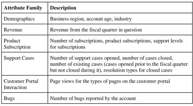
The dataset included 103 features (the attribute families of the 103 features are described in Table 1), thus indicating this project could benefit from dimensionality reduction. The Scikit learn module offers built-in methods for both feature selection and dimensionality reduction, four of which are relevant for the current project: (1) removing features with low variance; (2) feature agglomeration; (3) random projection; and (4) feature agglomeration.
Removing features with low variance is a filter technique for attribute subset selection method. Features with low variance (that is, variance close to 0) tend to have very little predictive value and thus can, in many cases, be discarded. Features with variance below 0 will be removed prior to analysis.
Random projection (RP) reduces the dimensionality of data by trading a controlled amount of error for faster processing times and smaller model sizes, while approximately preserving the pairwise distances between any two samples (Pedregosa et al., 2010). This project will use Scikit-learn's implementation of sparse random
projection.
Principal component analysis (PCA) is linear dimensionality reduction that transforms a set of observations into a set of values of linearly uncorrelated variables called principal components. This project will use PCA using Minka's MLE to guess the dimension and full singular value decomposition (SVD) as parameters.
Table 1: Attribute families
Attribute Family Description
Demographics Business region, account age, industry Revenue Revenue from the fiscal quarter in question Product
Subscription
Number of subscriptions, product subscriptions, support levels for subscriptions
Support Cases Number of support cases opened, number of cases closed, number of existing cases (cases opened prior to the fiscal quarter but not closed during it), resolution types for closed cases
Customer Portal Interaction
Page views for the types of pages on the customer portal
Bugs Number of bugs reported by the account
Algorithms
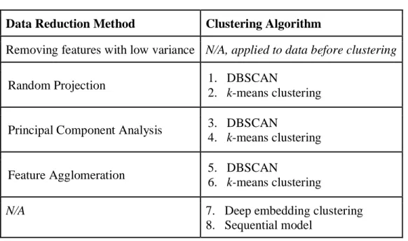
of which are implemented using the Keras API in Python. DEC is a method proposed and built by Xie, Girshick, & Farhadi, 2016 in which deep neural networks are used to learn the feature representations and cluster assignments simultaneously. Table 2 summarizes the testing framework for this project.
Table 2: Testing Framework
Data Reduction Method Clustering Algorithm
Removing features with low variance N/A, applied to data before clustering
Random Projection 1. DBSCAN
2. k-means clustering Principal Component Analysis 3. DBSCAN
4. k-means clustering
Feature Agglomeration 5. DBSCAN
6. k-means clustering
N/A 7. Deep embedding clustering
8. Sequential model
Evaluation
Results
Data
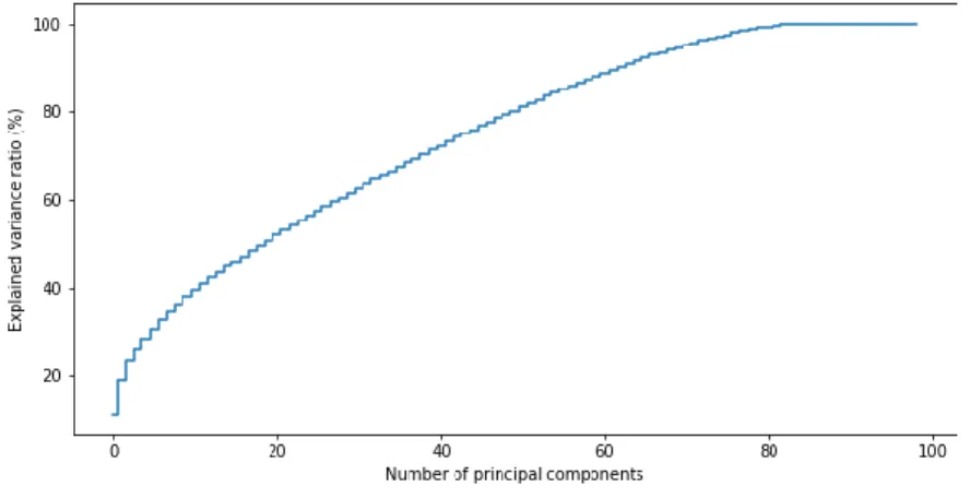
There were 105,632 accounts and 103 features included in the dataset. The calculated Hopkins statistic was 0.99, indicating a high clustering tendency. An analysis of the explained variance ratio showed that about 90% of the variance could be explained by about 80 principal components (features) (Figure 1).
Figure 1. Explained variance ratio by number of principal components
Dimensionality Reduction
analysis reduced the number of attributes to 98. The number of features in range (2,98) were recursively tested to identify the optimal number of attributes for random projection based on their effect on the silhouette scores for a k-means algorithm with n=3 clusters; the tests indicated that the optimal number of features on which to project the data was 7. The number of features in range (2,98) were recursively tested to identify the optimal number of attributes for feature agglomeration based on their effect on the silhouette scores for a k-means algorithm with n=3 clusters; the tests did not result in an optimal number of features as all silhouette scores were above 0.70 with little variance between them. Feature agglomeration was therefore not tested further.
Clustering Algorithms DBSCAN
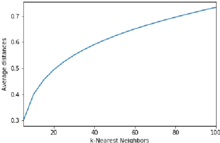
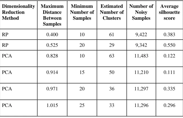
Two parameters required for DBSCAN are the epsilon value and minimum number of samples to be defined, where epsilon represents the maximum distance between two samples for them to be considered as being in the same neighborhood and the minimum number of samples refers to the number of samples in a neighborhood for a point to be considered a core point. An analysis of the average distances between
Figure 2: Average distances by k-Nearest Neighbors using RP
Figure 3: Averaged distances by k-Nearest Neighbors using PCA
Table 3: Summary of DBSCAN results Dimensionality Reduction Method Maximum Distance Between Samples Minimum Number of Samples Estimated Number of Clusters Number of Noisy Samples Average silhouette score
RP 0.400 10 61 9,422 0.383
RP 0.525 20 29 9,342 0.550
PCA 0.828 10 63 11,483 0.122
PCA 0.914 15 50 11,210 0.111
PCA 0.971 20 36 11,297 0.335
PCA 1.015 25 33 11,296 0.296
k-means
Figure 4: PCA-k-means explained variance by number of clusters
Figure 5: RP-k-means explained variance by number of clusters
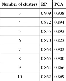
Table 4: Average silhouette scores by number of clusters and data reduction method
Number of clusters RP PCA
3 0.909 0.938
4 0.872 0.894
5 0.855 0.893
6 0.870 0.823
7 0.863 0.902
8 0.865 0.900
9 0.864 0.866
Outlier and Noise Detection and Analysis
Thus, it appeared that 3 was the optimal number of clusters. However, upon inspection, the clusters did not have even densities, with one cluster being composed of almost all the samples (~105,000), suggesting that outlier removal would be necessary to improve the results of the clustering. Using the data reduced via RP to decrease the memory and computation time required, the Isolation Forest algorithm for outlier detection was used to split the dataset into inliers and outliers. 10,563 samples (approximately 10% of the accounts) were labeled as outliers.
Additional testing using k-means clustering and DBSCAN was performed on both inliers and outliers. To reduce computation time, the inliers were reduced using RP, but the size of the outliers dataset was small enough for in-memory computation. The explained variance by number of clusters for inliers and for outliers using k-means are shown in Figure 6 and Figure 7, respectively. The corresponding silhouette scores by number of cluster are shown in Table 5; as the sample size for the outliers was so small, the actual silhouette score was calculated rather than the average.
Figure 7: Explained variance by number of clusters for outliers
Table 5: Silhouette scores by number of clusters for inliers versus outliers
Number of clusters Inliers Outliers
5 0.337 0.766
10 0.385 0.439
15 0.424 0.199
20 0.450 0.395
25 0.351 0.384
30 0.368 0.428
35 0.346 0.171
40 0.366 0.101
45 0.377 0.16
50 0.377 0.122
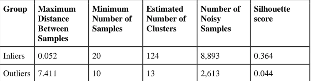
The analysis for inliers indicated that a 0.052 would be the optimal epsilon value, with a minimum number of samples of 20 (Figure 8). The analysis for outliers indicated that a 7.411 would be the optimal epsilon value, with a minimum number of samples of 10 (Figure 9). The results of the DBSCAN clustering are summarized in Table 6.
Figure 8: Average distances by k-nearest neighbors for inliers
Table6: DBSCAN results for inliers versus outliers
Group Maximum Distance Between Samples
Minimum Number of Samples
Estimated Number of Clusters
Number of Noisy Samples
Silhouette score
Inliers 0.052 20 124 8,893 0.364
Outliers 7.411 10 13 2,613 0.044
Testing with k-means algorithms where the number of clusters equals 3 for the inliers with and without noise and the outliers with and without noise indicated that further clustering would not be informative. The results are summarized in Table 7.
Table 7: Sub-clustering of inliers and outliers using k-means with three clusters
Group Silhouette Score Cluster sizes
Inliers All inliers 0.329 36083, 58971, 2
Non-noisy inliers 0.384 31191, 54971, 2
Noisy inliers 0.708 8821, 34, 37
Outliers All outliers 0.807 161, 1, 0
Non-noisy outliers 0.224 6537, 1376, 37
Noisy outliers 0.593 2478, 134, 0
Classification
Using the full data set labeled with the three clusters identified via the cluster analysis, the data were then fed into a classification algorithm to attempt to develop a predictive model to verify the results. The cluster breakdown is provided in Table 8.
Table 8: Cluster breakdown
Cluster Number of Samples
0 (inliers) 86,172
1 (noisy inliers) 8,893
2 (outliers) 7,950
3 (noisy outliers) 2,613
Table 9: Decision tree cross-validated accuracy (%)
Run Original Feature set Reduced Feature set
0 97.655 97.751
1 97.691 97.393
2 97.798 97.691
3 97.893 97.643
4 97.726 97.488
5 97.643 97.631
6 97.964 97.487
7 97.618 97.797
8 97.476 97.690
9 97.749 97.595
Average 97.721 97.617
Table 10: Confusion matrix of decision tree classifier
True
Predicted
Inlier Noisy inlier Outlier Noisy outlier
Inlier 8,561 397 26 0
Noisy inlier 128 8,641 91 4
Outlier 11 90 8,939 67
Noisy outlier 0 0 0 9,045
Deep Neural Networks
Both DNNs were trained on 70% of the data, and tested on the remaining 30%. The DEC converged at an accuracy of 70.692%, a normalized mutual information score of 0.380, and an adjusted Rand index of 0.432. A Sequential model with an input layer, two hidden layers, and three dropout layers (to reduce overfitting) converged with 100% accuracy and categorical hinge loss of 0.3021 and 0.2841 during training and validation,
Discussion
The customer accounts could not be clustered well using k-means despite a high clustering tendency; the results using DBSCAN suggest that a larger number of smaller clusters would better represent the data, however even these clusters overlap greatly. Separating the accounts into inliers and outliers, and identifying the noisy samples within both of those groups yielded more interesting results, as shown in Table 11.
Table 11: Resulting groupings of customer accounts
Group (n) Average
Revenue
Average
Account Age
in Days (SD)
Average # of
Support Cases
Opened (SD)
Average # of
Entitlements (SD) Average Portal Views (SD) Inlier (n=86,164) Low 1,282.22 (928.49)
0(0.01) 3.67(3.63) 15.52(41.58)
Noisy inliers (n=8,892)
Medium low
1,798.16 (981.59)
0(0.12) 7.24(5.93) 133.08(161.82)
Outlier (n=7,950)
Medium high
1,831.96 (1009.05)
0.09(0.85) 19.14(19.14) 480.47(619.19)
Noisy outliers (n=2,613)
High
2,117.85 (904.5)
5.66(20.47) 49.39(117.66)
2,375.72(2532 0.72)
of revenue and engaging a more with their accounts, including that they were more likely to respond to surveys. Further, the inliers tended to be closer together across features, as demonstrated by the standard deviations from the mean.
The attribute subset selection methods yielded mixed results for this project: removing features with low variance removed only 4 features, and PCA removed one additional feature. However, RP helped reduce the size of the dataset and thus yielded quicker computation times. However, both RP and PCA are a "black box" in that they do not provide information on which features were the most important in designating group membership. Decision Tree classifiers, on the other hand, assigns weights for each feature, which enabled the identification of the most important features; these features involved the amount of portal interactions and features around product subscriptions.
The results from testing with DNNs suggest that they can also provide answers to both clustering and classification problems with high-dimensional customer data… The clustering created by the DEC method resulted in high accuracy (70.692%), suggesting that the groupings as determined by the combined outlier and noise detection methods did exist with some underlying data structure. Similarly, the Sequential model resulted in high classification accuracy (100%), further suggesting that the groups do exist.
While the results were lukewarm, they confirmed what makes sense given the organization's subscription-based business model and can inform certain business decisions. For example, given that the outliers were more engaged with their
subscriptions, they would be prime candidates for providing feedback about products, support, and the design and functionality of the customer website through surveys, usability testing, and beta testing of new releases. Further, the information about the most important features from the results of testing with the decision tree classifier can help inform some of the additional, informal groupings of customer accounts which certain business units rely on to complete their day-to-day work.
Limitations
A number of tradeoffs had to be made regarding the data to complete the analysis. For example, certain data were restricted to only the previous fiscal quarter to reduce processing time given the exploratory nature of the task; however, it is possible that some of the features included in the dataset are seasonal, and thus, there may be some
seasonality to whether accounts are more or less similar. Even with the reduced size of the data, sampling was still required for certain calculations (e.g., silhouette scores) because of the size of the dataset. Lastly, the original selection of features was led by humans, that is, not all data on the accounts were included; it is possible certain features were not included that could have provided additional information for the clustering.
which affected the current analysis is that it does not recognize that different parts of the data could require different parameters—as evidenced by the different optimal values for epsilon and minimum samples required for the inliers versus the outliers (Berkhin, 2006); a nonparametric approach which does not assume uniform distribution may yield results which more accurately reflect the ground truth. Moreover, DNNs are subject to
overfitting data, and this could explain the high accuracy achieved using a Sequential model. Moreover, both DNN methods required labeled data; thus, both are subject to the limitations present in the grouping of the data as shown previously in Table 11.
Next Steps
The next steps for the current project are to expand the analysis by utilizing additional machine power to enable the inclusion of additional features, reduce the computation time, and improve the accuracy of calculations. Further, additional
algorithms which perform better with high-dimensional data should be tested to find the optimal clustering of accounts. For example, grid-based clustering, which can reduce the computation time, or subspace clustering, which can detect clusters in smaller subspaces of the data, may be viable options that fit the data better than the methods used in the current analysis; there were no available implementations of these methods in the modules used for this project and the time constraints did not permit creating an implementation.
likely have similar needs and considering the amount of overlap between the clusters, only small adjustments to the strategy would be required for each "level" of the clustering. Additionally, the four groupings of accounts from the outlier and noise
detection and analysis (inliers, noisy inliers, outliers, noisy outliers), can be used to focus efforts relating to feedback (e.g., through surveys or beta testing of new features) to a much smaller population of customer accounts who are demonstrably more likely to provide feedback as it is (outliers and noisy outliers). Lastly, the decision tree classifier used to verify the results of the four groupings could be further refined and developed to serve as a predictive model for new accounts; as a new account joins, the data about the revenue they will provide and the number and types of subscriptions for which they have subscriptions can be used to identify to which grouping they will likely fall into, and their experience can be tailored accordingly. For example, an account that has been identified as an outlier or noisy outlier could be followed more closely as they will be more likely to provide feedback; this can then inform the business strategy for engaging and
Conclusions
Customer segmentation, for which cluster analysis is a first step, is an important business question many organizations pose. The current project used customer account data from a software company to perform a cluster analysis to identify the potential for formal, data-driven customer segmentation that could be used across the business, rather than for one specific business unit. Given the high-dimensionality of the data and the exploratory nature of cluster analyses, multiple dimensionality reduction techniques and clustering algorithms were employed and tested, including DNNs.
In reviewing the resulting groupings of accounts, it was clear that, on average, the free and/or smaller-sized accounts tended to interact less with their subscriptions, and this group comprises the bulk of the businesses customers. Moreover, a much smaller
percentage of customers (10%) tended to not only generate more revenue, but also tended to interact more with their subscriptions on average. These results not only confirmed assumptions that many had about customer accounts based on the business model, but can also be used as is to inform certain business decisions. For example, the results from the DBSCAN clusters can inform a spectrum of customer support strategies that best fit the needs of the different clusters; the results from the outlier and noise detection and analysis can identify which accounts to target for feedback through surveys and beta testing; and the decision tree model can be used to predict the grouping to which a new account will likely belong when joining, which will inform the best strategy for
onboarding and retaining the new account.
Bibliography
Alelyani, S., Tang, J., & Liu, H. (2013). Feature selection for clustering: A review. Data Clustering: Algorithms and Applications, 29, 110-121.
de Amorim, R. C. (2016). A survey on feature weighting based K-Means algorithms. Journal of Classification, 33(2), 210-242.
Atkinson, A.C., Riani, M., & Cerioli, A. (2018) Cluster detection and clustering with random start forward searches, Journal of Applied Statistics, 45:5, 777-798, DOI: 10.1080/02664763.2017.1310806
Bair, E. (2013). Semi‐supervised clustering methods. Wiley Interdisciplinary Reviews: Computational Statistics, 5(5), 349-361.
Berkhin, P. (2006). A survey of clustering data mining techniques. (pp. 25-71). Berlin, Heidelberg: Springer Berlin Heidelberg. doi:10.1007/3-540-28349-8_2
Bingham, E., & Mannila, H. (2001). Random projection in dimensionality reduction: Applications to image and text data. KDD-2001: Proceedings of the Seventh ACM SIGKDD International Conference on Knowledge Discovery and Data Mining. New York: Association for Computing Machinery. pp. 245–250. doi:10.1145/502512.502546.
Bouveyron, C., Girard, S., & Schmid, C. (2007;2006;). High-dimensional data clustering. Computational Statistics and Data Analysis, 52(1), 502-519.
Chandrashekar, G., & Sahin, F. (2014). A survey on feature selection methods. Computers and Electrical Engineering, 40(1), 16-28.
doi:10.1016/j.compeleceng.2013.11.024
Dash M., & Koot P.W. (2009) "Feature Selection for Clustering". In Encyclopedia of Database Systems (pp. 1119-1125). Springer, Boston, MA
Dash, M., & Liu, H. (2000, April). Feature selection for clustering. In Pacific-Asia Conference on knowledge discovery and data mining (pp. 110-121). Springer, Berlin, Heidelberg.
Dy, J. G., & Brodley, C. E. (2004). Feature selection for unsupervised learning. Journal of machine learning research, 5(Aug), 845-889.
Eftekhari, A., Babaie-Zadeh, M., & Abrishami Moghaddam, H. (2011). Two-dimensional random projection. Signal Processing, 91(7), 1589-1603.
doi:10.1016/j.sigpro.2011.01.002
Guyon, I., & Elisseeff, A. (2003). An introduction to variable and feature selection. Journal of machine learning research, 3(Mar), 1157-1182.
Han, J., Kamber, M., & Pei, J. (2011a). Cluster Analysis: Basic Concepts and Methods. In Data mining: Concepts and techniques 3rd edition. San Diego, CA, USA: Elsevier Science.
Han, J., Kamber, M., & Pei, J. (2011b). Cluster Analysis: Basic Concepts and Methods. In Data mining: Concepts and techniques 3rd edition. San Diego, CA, USA: Elsevier Science.
Hunter, J.D. (2007) Matplotlib: A 2D Graphics Environment, Computing in Science & Engineering, 9, 90-95, DOI:10.1109/MCSE.2007.55
Jain, A. K. (2010). Data clustering: 50 years beyond K-means. Pattern Recognition Letters, 31(8), 651-666. doi:10.1016/j.patrec.2009.09.011
John, G. H., Kohavi, R., & Pfleger, K. (1994). Irrelevant features and the subset selection problem. In Machine Learning Proceedings 1994 (pp. 121-129).
Jones, E., Oliphant, E., Peterson, P., et al. SciPy: Open Source Scientific Tools for Python, 2001-, http://www.scipy.org/
Kambhatla, N., & Leen, T. K. (1997). Dimension reduction by local principal component analysis. Neural Computation, 9(7), 1493-1516. doi:10.1162/neco.1997.9.7.1493 Kane, D. M., & Nelson, J. (2014). Sparser johnson-lindenstrauss transforms. Journal of
the Association for Computing Machinery, 61(1), 4.
Kohavi, R., & John, G. H. (1997). Wrappers for feature subset selection. Artificial intelligence, 97(1-2), 273-324.
Kriegel, H., Kröger, P., & Zimek, A. (2009). Clustering high-dimensional data: A survey on subspace clustering, pattern-based clustering, and correlation clustering. ACM Transactions on Knowledge Discovery from Data (TKDD), 3(1), 1-58.
doi:10.1145/1497577.1497578
Krizhevsky, A., Sutskever, I., & Hinton, G. E. (2012). Imagenet classification with deep convolutional neural networks. In Advances in neural information processing systems (pp. 1097-1105).
Lu, Y., Cohen, I., Zhou, X. S., & Tian, Q. (2007). Feature selection using principal feature analysis. In Proceedings of the 15th ACM international conference on Multimedia (pp. 301-304). ACM.
Mckinney, W. (2010) Data Structures for Statistical Computing in Python, Proceedings of the 9th Python in Science Conference, (pp. 51-56).
Melnic, M. L. (2017). How to strengthen customer loyalty, using customer segmentation? Bulletin of the Transilvania University of Brasov. Series V : Economic Sciences, 9(2), 51-60.
Milligan, G. W., & Cooper, M. C. (1988). A study of standardization of variables in cluster analysis. Journal of Classification, 5(2), 181-204.
doi:10.1007/BF01897163
Modha, D. S., & Spangler, W. S. (2003). Feature weighting in k-means clustering. Machine Learning, 52(3), 217-237. doi:10.1023/A:1024016609528
Oliphant, T.E. (2006) A guide to NumPy, USA: Trelgol Publishing.
Parsons, L., Haque, E., & Liu, H. (2004). Subspace clustering for high dimensional data: A review. ACM SIGKDD Explorations Newsletter, 6(1), 90-105.
doi:10.1145/1007730.1007731
Pedregosa, F., Varoquaux, G., Gramfort, A., Michel, V, Thirion, B., Grisel, O., Blondel, M., Prettenhofer, P., Weiss, R., Dubourg, V., Vanderplas, J., Passos, A.,
Cournapeau, D., Brucher, M., Perrot, M., & Duchesnay, E. Scikit-learn: Machine Learning in Python, 2010-, http://scikit-learn.org/
Cournapeau, D., Brucher, M., Perrot, M., & Duchesnay, E. (2010) Scikit-learn: Machine Learning in Python, Journal of Machine Learning Research, 12, 2825-2830.
Rezaeinia, S. M., Keramati, A., & Albadvi, A. (2012). An integrated AHP-RFM method to banking customer segmentation. International Journal of Electronic Customer Relationship Management, 6(2), 153-168. doi:10.1504/IJECRM.2012.048721 Rezaeinia, S. M., & Rahmani, R. (2016). Recommender system based on customer
segmentation (RSCS). Kybernetes, 45(6), 946-961. doi:10.1108/K-07-2014-0130 Schmidhuber, J. (2015). Deep learning in neural networks: An overview. Neural
Networks, 61, 85-117. doi:10.1016/j.neunet.2014.09.003
Sembiring, R. W., & Zain, J. M. (2010). Cluster evaluation of density based subspace clustering. Journal of Computing, 2(11). Retrieved from
https://arxiv.org/pdf/1012.6009.pdf
Siniscalchi, S. M., Yu, D., Deng, L., & Lee, C. (2013). Exploiting deep neural networks for detection-based speech recognition. Neurocomputing, 106, 148-157.
doi:10.1016/j.neucom.2012.11.008
Song, M., Yang, H., Siadat, S. H., & Pechenizkiy, M. (2013). A comparative study of dimensionality reduction techniques to enhance trace clustering performances. Expert Systems with Applications, 40(9), 3722-3737.
doi:10.1016/j.eswa.2012.12.078
Upton, G., & Cook, I. (2014a). Distance measure. In A Dictionary of Statistics (3rd ed.). Oxford University Press.
Upton, G., & Cook, I. (2014b). Euclidean distance. In A Dictionary of Statistics (3rd ed.). Oxford University Press.
Upton, G., & Cook, I. (2014c). Overfitting. In A Dictionary of Statistics (3rd ed.). Oxford University Press.
Upton, G., & Cook, I. (2014d). Standardizing. In A Dictionary of Statistics (3rd ed.). Oxford University Press.
Witten, I. H., Frank, E., & Hall, M. A. (2011). Data mining: Practical machine learning tools and techniques (3rd ed.). San Diego, CA, USA: Elsevier Science.
Yu, W., Sun, X., Yang, K., Rui, Y., & Yao, H. (2018). Hierarchical semantic image matching using CNN feature pyramid. Computer Vision and Image
Understanding, 169, 40-51. doi:10.1016/j.cviu.2018.01.001
Xie, J., Girshick, R., & Farhadi, A. (2016, June). Unsupervised deep embedding for clustering analysis. In International conference on machine learning (pp. 478-487).
Glossary
Term Definition
artificial neural network (ANN)
a system that attempts to solve problems by pattern recognition, mimicking the activities and
representation of neuronal networks like those in the human brain
attribute subset selection (or feature selection or variable elimination)
a process of reducing the size of a dataset by removing irrelevant or redundant attributes
clustering (or cluster analysis)
a type of data mining task whose goal is to discover natural groupings (clusters) in a data set, as well as the process of building the models that represent these groupings
clustering tendency
refers to whether the dataset lends itself to being clustered; datasets that have a random structure are unlikely to cluster, whereas data with a non-random structure have a higher probability of clustering in meaningful ways
coclustering (or biclustering) refers to a clustering method in which both data points and their attributes are clustering simultaneously correlation-based clustering refers to a clustering method in which clusters are
defined by advanced correlation methods cross-validation
refers to the process of using involves a training set to training multiple models and comparing the quality of the models by their performance on a test set
customer segmentation the process of dividing the customer base into distinct and internally homogenous groups
curse of dimensionality
the idea that the large number of input variables and high volume of data may muddle the analysis and result in a model that overfits the data
data mining
deep learning
refers to non-task-specific machine learning methods whose goals are to learn about the underlying data representations with multiple levels of abstraction deep neural network refers to an artificial neural network with multiple hidden layers between the input and output layers density-based clustering
refers to a clustering method that will continue to grow a cluster as long as the density (the number of objects) in the cluster exceeds some threshold
distance measure (or distance metric)
a quantitative measurement of the distance between the points in multidimensional space
Euclidean distance the “straight-line" distance between two points
feature agglomeration
refers to the dimensionality reduction method that involves recursively merging features using a predefined calculation (e.g., mean) until the
predetermined number of feature clusters is reached feature construction
a step of data analysis that involves making decisions about which characteristics of the data to include and the best ways to represent these characteristics
grid-based clustering
refers to a clustering method that renders the object space into a grid composed of a finite number of cells; the clustering operations are performed on the grid space
hard clustering refers to a clustering model in which clusters are mutually exclusive
hierarchical clustering refers to a clustering method that creates a hierarchical decomposition of the set of data objects
Hopkins statistic a statistic that can be used to measure the clustering tendency of a dataset
inter-cluster variance variance of the data points in between clusters intra-cluster variance (or
within-cluster variance) variance of the data points in a cluster overfit
a model that overfits the data is unnecessarily
complicated and will likely perform poorly when faced with new data
principal component analysis (PCA)
random projection (RP)
refers to the transformation of a set of input data onto a lower-dimensional space while preserving the pairwise Euclidean distances
projected clustering
refers to a clustering method in which each data point is assigned to exactly one subspace cluster, and then a projection for where the points best cluster is found similarity measure
a metric used to quantify the distance between two data points and to determine how similar or dissimilar clusters are
semi-supervised learning
machine learning task in which the data used for analysis are partially labeled or when there are known constraints on how the data should be clustered soft clustering (or fuzzy
clustering)
refers to a clustering model in which data points are assigned probabilities of belonging to one cluster over another
standardization
the process of transforming the values of a variable such that the mean is centered at 0 with a standard deviation of 1
subspace clustering refers to a clustering method in which clusters can exist in multiple, possibly overlapping subspaces
supervised learning machine learning task in which the data used for analysis are not labeled