Sharif University of Technology
Scientia IranicaTransactions A: Civil Engineering http://scientiairanica.sharif.edu
Mode choice and number of non-work stops during the
commute: Application of a copula-based joint model
A. Rasaizadi
and M. Kermanshah
Department of Civil Engineering, Sharif University of Technology, Tehran, P.O. Box 9313-11155, Iran. Received 28 November 2015; received in revised form 30 September 2016; accepted 12 November 2016
KEYWORDS Joint model; Copula; Mode choice; Number of stops; Trip chain; Work trips.
Abstract. Commute mode choice and number of non-work stops during the commute are joint decisions interacting with each other. If an individual chooses a vehicle for the commute, regarding vehicle's restrictions, there could be some stops. On the other hand, if an individual needs to have some stops, a vehicle can be selected for the commute regarding the number of stops. In this study, to consider the interaction between these decisions, we employed a copula-based joint modeling framework. The data used in this study are drawn from origin-destination travels data of Shiraz-Iran conducted in 1997. The commuting mode choice modeling is undertaken using a multinomial logit model, and the number of non-work stops is modeled using an ordered response formulation. To capture the interaction between these decisions, several copula functions have been used. Results conrm that the mode and number of non-work stop choices are interrelated choices by estimating the commonly observed factors and dependence parameters with high statistical signicance. By determining common eective factors, we can analyze the current situation in the community. Therefore, we can use the results so as to forecast future travel demand and set some policies, leading to the promotion of trip chaining.
© 2018 Sharif University of Technology. All rights reserved.
1. Introduction
The continual growth of urban travels, in particular, traveling with the private vehicle, is one of the major reasons causing urban trac congestion and related problems such as noise and environmental pollutions, energy waste, and safety decline [1]. As the quality of human life improves, more comfort and convenience come along; in terms of a travel behavior scope, this leads to the increasing use of personal vehicle. Under such conditions, changing transportation
infrastruc-*. Corresponding author. Fax: +98 21 66014828
E-mail addresses: Arash [email protected] (A. Rasaizadi) [email protected] (M. Kermanshah).
doi: 10.24200/sci.2017.4194
tures is necessary to service the vehicles [1]. The high cost of constructions and operations necessitates a planner to nd better options. There are policies and planning along with the development of trans-portation infrastructures that could meet the future requirements.
To solve trac congestion, we must determine factors causing this problem. Work and educational trips constitute a major part of trac congestion in the morning and evening during peak hours. The home-to-work-trip trac congestion occurs during the morning peak hours, and the work-to-home-commute trac congestion occurs during the evening peak hours. Work and educational trips constitute a major share of people's trip. These trips are considered as manda-tory ones that, principally, could be not eliminated. For mandatory trips, we can induce conditions that
facilitate trac congestion reduction, e.g. promoting planned trip chain and improving public transportation eciency.
Usually, when people face trac congestion, they look for greater use of their travel. For example, instead of two separated trips to work and markets, they add stops in their work trip and do the shopping while cancelling their shopping trip. This idea is the basis for the formation of the trip chaining. The trip chain is a set of trips that people with the intention of making some stops would obtain their secondary goals in their main trip. In the rest of this paper, work and educational trips are considered as the work trip. This study examines work trip chains that have at least one non-work stop.
According to the above points, having more non-work stops during the commute and using public transport can reduce trac congestion, signicantly. Achieving several goals during the commute needs spending more time, and using public transport adds to the time spent [2]. Therefore, it can be expected that private vehicle utilization is more favorable and likely in such conditions [2]. This point indicates the complexity of the planning.
The rest of this paper is structured as follows. The next section provides a literature review. Section 3 discusses the methodology. Section 4 describes the data source. Section 5 reports results. Conclusions are reported in the nal section.
2. Literature review
Some earlier studies ignore the interaction between the commute mode and number of non-work stops [3-5]. Several studies are focused on the analysis of the number of stops without considering the eect of the commute mode [3,4]; on the contrary, a large number of studies are focused on the commute mode choice with no regards to the eect of the number of stops [5].
Some others have attempted to establish a tenu-ous link between stop-making and mode choice using one variable as an independent variable to describe an-other variable [6-8]. For example, Bhat and Sardesai [7] utilized the number of stops and travel time reliability as independent variables in the commute mode choice model. As an example, Strathman et al. [8] used trip characteristic, such as a commute mode, in the number of stops model. Some studies considered the interaction between commute mode choice and the number of stops and used joint modeling formulation; however, commute stops model is represented as a binary choice (no commute stops and one or more stops) [9,10].
Bhat [2] used an econometric structure for joint modeling of commute mode choice and the number of non-work stops where the number of stops can obtain any positive and integer values. The number
of stops is modeled using an ordered logit model, while the commute mode choice is modeled using a multi-nominal logit model. In this study, the key point is nding the joint probability function. In other words, for each individual, we must determine the joint probability of choosing the combination of each mode and each number of stops. According to the observation, the likelihood function is formed and maximized. Bhat formed a bivariate joint distribution as follows [2]:
- Error terms of commute mode choice follow the Gumbel distribution. Its cumulative distribution is calculated. By using normal inverse cumulative distribution, Gumbel distribution is converted into a normal distribution;
- Error terms of the number of stops follow the normal distribution;
- By using the bivariate normal distribution, joint bivariate distribution of error terms and joint prob-ability function are computed.
These methods can consider the interaction be-tween decisions, but restricting the relationship to one form is inappropriate. There are other functions that may be more appropriate to describing this correlation. Such functions are known as copulas. The copula is a function that generates a stochastic dependence relationship among random variables with pre-specied marginal distributions [1].
Finally, Bhat et al. [1] used copula in joint modeling of the commute mode choice and the number of stops during the commute. The data used in this study are drawn from the time-use multi-purpose survey conducted between 2002 to 2003 in a greater Turin metropolitan area of Italy. Mode choice model includes four choices: drive alone, shared ride, active transport, and public transport. the Number of stops includes 0, 1, 2, and more than 2 stops.
Frank and Gaussian copulas are used for joint modeling. The best model is obtained by the Gaus-sian copula that has log-likelihood equal to {1652.39. Results conrm the interaction between the two deci-sions [1].
The existence of some common observed and unobserved factors between these decisions indicates that these decisions are not separated and are not given priority. Some previous studies have considered the priority of these decisions. By using copula-based joint model, this study removed this priority. This paper used this methodology for joint modeling of mode choice and the number of non-work stops for the Iranian community using travel data of shiraz. Determining elasticity for dummy and ordered variable is considered as another novelty of this paper.
3. Methodology
This paper employed a copula-based joint model to recognize the factors with simultaneous eects on mode choice and the number of non-work stops. Some visible factors have common eects on mode choice and number of non-work stops. These factors are considered as commonly observed factors. Therefore, by obtaining knowledge about common factors, we can set some policies to increase the probability of choosing public transport and have more non-work stops during the commute facilitating trac congestion reduction. Further, there are some common unobserved factors between the two choices whose eects are undetectable by us in a systematic way. Therefore, the current paper employed some copula functions to consider the correlation between unobserved factors of the two models.
The commute mode choice is modeled using multinomial logit formulation. Assume that error terms of utility functions are identically and independently Gumbel distribution. The ordered-logit formulation is adopted for the number of non-work stops model. Assume that error terms of propensity function have a standard logistic distribution. Assumptions have been made on the basis of earlier studies' assumptions [1]. In this study, FGM, AMH, Frank, Gaussian, Gumbel, and Product copulas have been used to obtain a better tted model. The copula with the greatest log-likelihood and dependence parameters in an acceptable range is the best copula.
3.1. Model structure
The commute mode choice was modeled using a multi-nomial logit model. Let q be the index for individuals and i be the index for the mode. Let hqj be the latent
utility acquired by individual q for choosing travel mode i [11]:
hqi= xqi+ "qi; (1)
where xqi is the column vector of exogenous variables
specied to mode i, and is the corresponding column vector of parameters to be estimated. "qi represents
an idiosyncratic error term [2]. Assume that "qi
values are identically and independently extreme values distributed with the location parameter of zero across alternative i and individual q [2]. According to utility theory, individual q selects alternative i if and only if the following condition holds [11]:
hqi> maxj6=i hqi: (2)
Let rqi be a dummy variable; rqi = 1 if the ith mode
is chosen by the qth individual; rqi = 0 otherwise.
Dene [11] as in the following: vqi=
max
j6=i hqj
"qi: (3)
By combining Eqs. (1) and (2):
xqi+ "i> maxj6=i hqj: (4)
Eq. (4) can be rewritten as follows:
xqi> maxj6=i hqj "qi: (5)
Therefore, rqi= 1 if and only if xqi> vqi.
The implied marginal distribution of vqi can be
obtained through Eq. (3) and the distribution assump-tion on "qias follows [11]:
Fi(xqi) = Pr(vqi< Xqi) = Pexp(xqi) j exp(xqj)
;
j = 1; 2; : : : ; J: (6) The ordered logit formulation was used for the number of commute stops [1]. Let s
qirepresent the stop-making
propensity of the qth individual that uses mode i. sqi
is the number of non-work stops depending on mode choice i. sqi is observed only for the chosen mode i in
the sample [1]. Then, in the usual ordered response structure, we may write the following [1]:
s
qi= zqi+ qi; sqi= k; if i;k 1< sqi; (7)
where zqiis the column vector of the exogenous variable
specied to mode I, and is the corresponding column vector of coecients to be estimated. qi represents an
idiosyncratic error term assumed to be a standard logis-tic distributed with marginal cumulative distribution function G(:). terms are the threshold bounds that horizontally partition the latent stop-making propen-sity and provide the relationship between the latent stop-making propensity and the observed number of stops. By convention, i;0 = 1 and i;K = +1 for
each mode i, where k is an index for number of stops (k = 1; 2; 3; :::; K) [1]. The probability of individual q choosing mode i and making k commute stops is written as follows:
Pr[rqi=1; sqi= k] = Pr[vqi< xqi;
i;k 1 zqi< qi< i;k zqi];
Pr[rqi=1; sqi= k] = Pr[vqi< xqi; qi< i;k zqi]
Pr[vqi< xqi; qi< i;k 1 zqi]: (8)
To obtain this probability function, we need a bivariate cumulative distribution function between error terms of the two models. Therefore, copula functions were used. An m-copula can be dened as m-dimensional CDF whose support is contained in [0,1] and whose one-dimensional marginal is uniform on [0,1] [12]:
Table 1. Some copula characteristics.
Copula C(u1; u2) Dependence
parameter range
Product u1; u2 {
FGM u1u2(1 + (1 u1) (1 u2)) [{1,1]
Gaussian G 1(u1) ; 1(u2) ; ({1,1)
Clayton (u1 + u2 1) 1 (0; 1)
Frank 1log1 + (e u1 1)(e u2 1) e 1
( 1; 1)
Gumbel exp( (~u
1+ ~u2)1= [1; 1)
AMH u1u2(1 (1 u1)(1 u2)) 1 [{1,1]
Figure 1. owchart of methodology.
F (x1; : : : ; xm) = F (F1 1(u1); : : : ; Fm1(um))
= Pr[U1 u1; : : : ; Um um]
= C(u1; : : : ; um; ); (9)
where is the parameter of copula called the de-pendence parameter, which measures the dede-pendence between the marginals [12].
Eq. (8) can be rewritten using copula as follows: Pr[rqi=1; sqi= k] = C(uqi1; uqi;k;2)
C(uqi1; uqi;k 1;2); (10)
where dependence parameter () shows the correlation between vqi and qi. According to Eq. (3), the
correlation between "qi and qihas an inverse sign.
Table 1 shows characteristics of some copulas [12]. For more information, see [12-14].
3.2. Estimation procedure
Let 1[.] be an indicator function taking the value of unity if the expression in parenthesis is true, and 0 otherwise. Also, the following dummy variable is dened as follows [1]:
Mqik = 1[rqi= 1] 1[sqi= k]: (11)
The log-likelihood function for the estimation of pa-rameters in the model takes the following form [1]:
log L =
Q
X
q=1
XI
i=1 K
X
k=1
Mqiklog[Pr(rqi=1; sqi=k)]
: (12)
All parameters in the model are consistently estimated by maximizing the log-likelihood function. The pa-rameters estimated in the joint model are (k 1)i;k,
and vectors, and dependence parameters of the best tted copula. Maximization task is accomplished using R-studio programming. To do so, numerical methods are used to maximize log-likelihood function. Through an iterative process, convergence of answers could be achieved. Figure 1 shows the owchart of the methodology.
4. Data source
The source of data used in this study is derived from the origin-destination travel data of Shiraz-Iran conducted in 1997 by Sharif University of Technology, Iran for Transportation Studies and Research (ITSR). The survey collected data from 51212 peoples aged 6 years and older. The sample used in this paper includes 1029 individuals.
Work trip chains should have at least one non-work stop during the commute. Consider a situation where an individual has a trip from home toward work and coming back home. If an individual has at least one work trip and has one or more non-work stops, this set of trips is considered as the work trip chain. Also, the educational trip is considered as the work trip. An individual may use a variety of vehicles in his or her work trip chain. In this study, the mode used for the nal leg to work is used as the work trip chain mode [1]. Five dierent modes were selected for the MNL
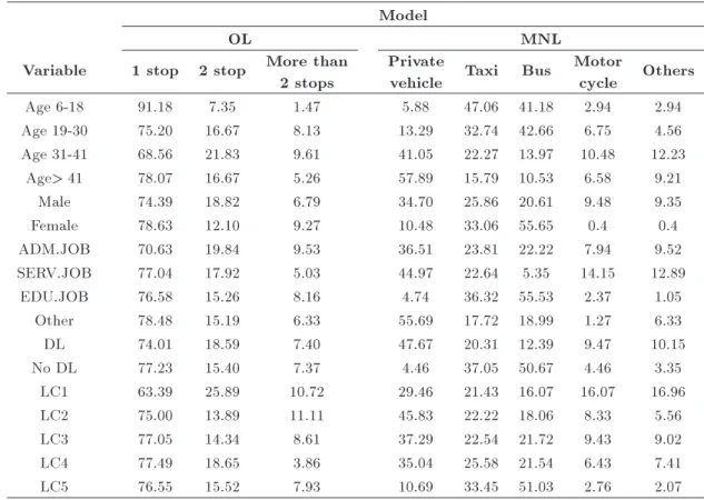
model. These modes are private vehicle, taxi, bus, motorcycle, and other. Table 2 shows commute modes' frequency. Frequency of number of stops is presented in Table 3. Table 4 introduces exogenous variables and Table 5 shows the distribution of data by the commute mode and by number of stops for exogenous variables.
Table 2. Commute mode frequency. Mode Frequency Frequency
percentage Private vehicle 297 28.86
Taxi 281 27.31
Bus 302 29.35
Motorcycle 75 7.29
Other 74 7.19
Total 1029 100
Table 3. Stops number frequency. Number of stops Frequency Frequency
percentage
1 776 75.41
2 177 17.20
More than 2 76 7.39
Total 1029 100
5. Results
Modeling is accomplished with our prior knowledge about the relationship between dependent and inde-pendent variables. An appropriate model is a model that has the biggest log-likelihood and has logical statistically signicant coecients. To investigate the matter, dierent copulas are examined.
In MNL model, the private vehicle is considered as the base mode and has zero utility [1]. Utility co-ecients of other modes are estimated comparatively. Age, job, and life cycle group of variables have one dummy variable as the base variable. Table 6 shows the general information about modeling with dierent copulas.
The best tted model is obtained by Frank copula that has a log-likelihood value of {1849.210, as com-pared to {1853.150 for product (independent) copula. Table 7 shows the joint modeling results with Frank copula.
5.1. Mode choice results
The coecients of the socio-demographic variables are presented favorably as expected. For example, for individuals with the driving license, a private vehicle is practically more advantageous than a taxi, bus, motorcycle, and others are. Increasing the number
Table 4. Exogenous variables.
Information Variables Denition percentageFrequency
Age
Age 6-18 = 1 if age is between 6 to 18, = 0 otherwise 6.61 Age 19-30 = 1 if age is between 19 to 30, = 0 otherwise 48.98 Age 31-41 = 1 if age is between 31 to 41, = 0 otherwise 22.25 Age> 41 = 1 if age is over than 41, = 0 otherwise 22.16
Sex Sex =1 for males, 0 = for females 75.90
Job
ADM.JOB = 1 if individual has an administrative job, = 0 otherwise 24.49 SERV.JOB = 1 if individual has a service job, = 0 otherwise 30.90 EDU.JOB = 1 if individual has an educational job, = 0 otherwise 36.93 Other = 1 if individual has another job, = 0 otherwise 7.68 Driving license DL = 1 if individual has a driving license, 0 = otherwise 56.46
Number of
vehicle NVEH Number of vehicle {
Household size HHSZ Household size {
Lifecycle
LC1 = 1 if individual belongs to family in life cycle 1, = 0 otherwise 10.88 LC2 = 1 if individual belongs to family in life cycle 2, = 0 otherwise 7.00 LC3 = 1 if individual belongs to family in life cycle 3, = 0 otherwise 23.72 LC4 = 1 if individual belongs to family in life cycle 4, = 0 otherwise 30.22 LC5 = 1 if individual belongs to family in life cycle 5, = 0 otherwise 28.18
* a) Families with the oldest child under 6 years; b) Families with the oldest child between 6 and 11 years; c) Families with the oldest child between 12 and 18 years;
d) Families with at least one child over 18 and youngest child under 18; e) Other types of families [16,17].
Table 5. Distributions by commute mode and by number of stops for exogenous variables. Model
OL MNL
Variable 1 stop 2 stop More than 2 stops
Private
vehicle Taxi Bus
Motor
cycle Others
Age 6-18 91.18 7.35 1.47 5.88 47.06 41.18 2.94 2.94
Age 19-30 75.20 16.67 8.13 13.29 32.74 42.66 6.75 4.56
Age 31-41 68.56 21.83 9.61 41.05 22.27 13.97 10.48 12.23
Age> 41 78.07 16.67 5.26 57.89 15.79 10.53 6.58 9.21
Male 74.39 18.82 6.79 34.70 25.86 20.61 9.48 9.35
Female 78.63 12.10 9.27 10.48 33.06 55.65 0.4 0.4
ADM.JOB 70.63 19.84 9.53 36.51 23.81 22.22 7.94 9.52
SERV.JOB 77.04 17.92 5.03 44.97 22.64 5.35 14.15 12.89
EDU.JOB 76.58 15.26 8.16 4.74 36.32 55.53 2.37 1.05
Other 78.48 15.19 6.33 55.69 17.72 18.99 1.27 6.33
DL 74.01 18.59 7.40 47.67 20.31 12.39 9.47 10.15
No DL 77.23 15.40 7.37 4.46 37.05 50.67 4.46 3.35
LC1 63.39 25.89 10.72 29.46 21.43 16.07 16.07 16.96
LC2 75.00 13.89 11.11 45.83 22.22 18.06 8.33 5.56
LC3 77.05 14.34 8.61 37.29 22.54 21.72 9.43 9.02
LC4 77.49 18.65 3.86 35.04 25.58 21.54 6.43 7.41
LC5 76.55 15.52 7.93 10.69 33.45 51.03 2.76 2.07
Table 6. General information about modeling with dierent copulas. Copula Acceptable
range for
Dependent parameters Acceptable
models
Log-likelihood Private vehicle Taxi Bus Motor Others
Frank ( 1; 1) 1.236 0.600 2.031 1.422 1.661 p {1849.21
Product { { { { { { p {1853.15
Gumbel [1,1) 1.123 1.030 1.208 1.163 1.226 p {1849.34
Gaussian ({1,1) {2.448 {1.312 8.376 5.456 {5.094 {
FGM [{1,1] 1.516 0.753 1.396 0.985 1.276 {
AMH [{1,1] 1.334 0.575 1.232 0.860 1.143 {
of private vehicle ownership causes more favorability of private vehicle than other modes. As individual age increases, public transport (bus and taxi) loses its utility, and private vehicle utility increases instead. Further, motorcycle and others have more practical advantage for men rather than women.
5.2. Number of non-work stops results
Similar to the mode choice, numbers of non-work results are sucient as expected. Individuals in 6-18 years old groups have a lower propensity for more non-work stops. Also, men have a higher propensity for more non-work stops rather than women. People in life cycle 1 have a higher stop-making propensity than other life cycle groups. Results show that driving
li-cense, the number of vehicle ownership, and household size do not have any eects on the number of non-work stops.
5.3. Correlation parameters
Dependence parameters of each mode are signicantly dierent from zero, indicating a positive correlation among common unobserved factors related to both mode choice and the number of non-work stops, specif-ically between error terms vqi and qi. The positive
dependence parameters indicate a negative correlation between utility error term ("qi) and propensity error
term (qi). These negative correlations are
inter-pretable. For example, a workplace in the central busi-ness district is an unobserved factor that increases stop
Table 7. Joint modeling results with frank copula.
Variable MNL OL
Private vehicle Taxi Bus Motor cycle Others Dependence parameters
Private vehicle { - { { { 1.237 (1.216)
Taxi { { { { { 0.600 (0.706)
Bus { { { { { 2.031 (2.075)
Motorcycle { { { { { 1.423 (1.551)
Other { { { { { 1.662 (1.652)
Constants - 2.419 1.485 {2.530 {0.963 {1.807
(5.145) (3.132) ({2.301) ({0.890) ({4.300)
Age 6-18 (base) - - -
-Age 19-30 - - 0.481 1.006 - 1.365
(2.095) (3.316) (3.052)
Age 31-41 - {0.611 - - - 1.800
({2.406) (3.668)
Age > 41 - {1.130 {0.432 - {0.638 1.376
({3.982) ({1.368) ({2.162) (2.721)
Sex - - {0.223 2.595 2.422 0.355
({1.274) (2.526) (2.361) (1.746)
SERV.JOB (base) - - -
-ADM.JOB - - 1.514 - - 0.417
(4.986) (2.269)
EDU.JOB - 0.743 2.424 - {1.022 0.587
(2.343) (6.462) ({1.703) (2.366)
Others - {0.441 1.037 {2.087 -
-({1.224) (2.368) ({2.035)
DL - {1.879 {2.339 {1.712 {1.432
-({6.117) ({7.373) ({4.648) ({3.476)
NVEH - {1.553 {1.479 {0.358 {1.191
-({7.651) ({7.006) ({1.480) ({4.467)
-HHSZ - {0.132 - - -
-(2.519)
LC1 - {0.424 {0.736 0.588 - 0.622
({1.259) ({2.051) (1.676) (2.837)
LC2 - - - - {1.090
-({1.999)
LC3 - - - 0.554 -
-(1.723)
LC4 (base) - - -
-LC5 - 0.410 - - -
-(1.621)
Threshold 1-2 stops - - - 0.999
(4.928)
Threshold 2-3 stops - - - 2.414
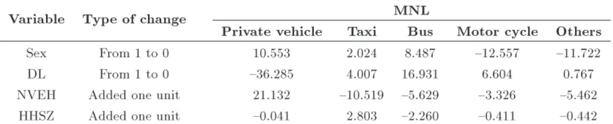
Table 8. Aggregate elasticity for some dummy and ordinal variables.
Variable Type of change MNL
Private vehicle Taxi Bus Motor cycle Others
Sex From 1 to 0 10.553 2.024 8.487 {12.557 {11.722
DL From 1 to 0 {36.285 4.007 16.931 6.604 0.767
NVEH Added one unit 21.132 {10.519 {5.629 {3.326 {5.462
HHSZ Added one unit {0.041 2.803 {2.260 {0.411 {0.442
propensity due to the presence of many opportunities in these districts and private vehicle utility decreases, because there is condensed trac in these districts. It can be used to interpret a negative correlation among private utility and stop-making propensity error terms. The statistical signicance of dependence parame-ter is in accordance with the expectations and previous research results. This point can be used to validate the model.
5.4. Elasticity
Elasticity is a concept that can be employed for continuous variables. There is no continuous variable in the exogenous variable set. To determine the aggregate elasticity for dummy and ordinal variable, the following measure has been taken [15]:
- For dummy variables, we change one values to zero and zero values to one. Then, the absolute shifts in the expected share are summed up;
- For ordinal variables, we increase variables by one and compute expected shifts.
This elasticity is disaggregating. To determine aggregate elasticity, we use [11]:
ExiP (i)=
N
P
n=1Pn(i) EPn
xin(i)
N
P
n=1Pn(i)
; (n = 1; :::; N); (13)
where EPn(i)
xin is the disaggregate elasticity for xi
vari-able, i is the mode choice, and Pn(i) is the probability
of mode i chosen by individual n.
Table 8 shows the aggregate elasticity for some dummy and ordinal variables.
6. Conclusion
In this study, the interaction between commute mode choice and the number of non-work stops was examined in the copula-based joint model framework. The existing common or related observed and unobserved factors between the two models were captured by joint modeling. The copula function was used to combine unobserved factors of models and approved results
of these correlations through estimating signicant parameters statistically for copula dependence. This model can be used in two ways: to predict future travel demands of society and have an appropriate planning to respond; to use the results to set policies for the current situation so as to reduce trac congestion. Those factors that increase the probability of using public transport and having more non-work stops should be supported. The important point is that these results, while validated, are viable for Shiraz only, not for anywhere else.
References
1. Portoghese, A., Bhat, C.R., and Eluru, N. \A copula-based joint model of commute mode choice and number of non-work stops during the commute", Transporta-tion Research Part B, 38(3), pp. 337-362 (2011).
2. Bhat, C.R. \Work travel mode choice and number of non-work commute stops", Transportation Research Part B, 31(1), pp. 41-54 (1997).
3. Cao, X., Mokhtarian, P.L., and Handy, S.L. \Dieren-tiating the inuence of accessibility, attitudes, and de-mographics on stop participation and frequency during the evening commute", Environment and Planning B, 35(3), pp. 431-442 (2008).
4. Chu, Y.L. \Empirical analysis of commute stop-making behavior", Transportation Research Record: Journal of the Transportation Research Board, 1831, pp. 106-113 (2003).
5. Lizana, P., Arellana, J., Ortuzar, J.D., and Rizzi, L.I. \Modeling mode and time-of-day choice with joint RP and SC data", International Choice Modelling Conference, Sydney, Australia (2013).
6. Ye, X., Pendyala, R.M., and Gottardi, G. \An explo-ration of the relationship between mode choice and complexity of trip chaining patterns", Transportation Research Part B, 41(1), pp. 96-113 (2007).
7. Bhat, C.R. and Sardesai, R. \The impact of stop-making and travel time reliability on commute mode choice" Transportation Research Part B, 40(9), pp. 709-730 (2006).
8. Strathman, J.G., Dueker, K.J., and Davis, J.S. \Ef-fects of household structure and selected travel charac-teristics on trip chaining", Transportation, 21(1), pp. 23-45 (1994).
9. Hensher, D.A. and Reyes, A.J. \Trip chaining as a barrier to the propensity to use public transport" Transportation, 27(4), pp. 341-361 (2000).
10. Damm, D. \Interdependencies in activity behavior", Transportation Research Record: Journal of the Trans-portation Research Board, 750, pp. 33-40 (1980).
11. Ben-Akiva, M.E. and Lerman, S., Discrete Choice Analysis: Theory and Applications to Travel Demand, MIT Press (1985).
12. Trivedi, P.K. and Zimmer, D.M., Copula Modeling: an Introduction for Practitioners, Now Publishers Inc (2007).
13. Piotr, J., Durante, F., and Hardle, W.K., Copula in Mathematical and Quantitative Finance, Springer (2012).
14. Nelsen, R.B., An Introduction to Copulas (2nd Ed.), Springer (2006).
15. Daly, A. and Hess, S. \Simple approaches for random utility modeling with panel data", TRB Annual Meet-ing, Washington DC (2013).
16. Owen, D., Yilin, S., and Octavious, S.Y. \Designing low carbon cities with a family lifecycle in mind: Where should our focus be?" TRB Annual Meeting, Washington DC (2014).
17. Sun, Y., Huang, Z., and Kitamura, R. \Travel be-havior, household in the same life cycle stage", Built Environment, ICTE, pp. 1-6 (2011).
Biographies
Arash Rasaizadi obtained his BSc degree in Civil En-gineering from Shahid Bahonar University of Kerman, Kerman, Iran in 2013; he also received his MSc degree in Transportation Engineering from Sharif University of Technology, Tehran, Iran in 2015. He is currently a PhD student in the Transportation Planning in Tarbiat Modares, Tehran, Iran. His research interests include forecast and management of urban travel demand, transportation behavior, and urban transportation planning.
Mohammad Kermanshah received his BS degree in 1974 from Shiraz University, Iran, his MS degree from South Dakota School of Mines & Technology in USA in 1978, and his PhD degree from the University of Davis, California, USA in 1984. He is now a Professor of Civil Engineering at Sharif University of Technology, Tehran, Iran. His research interests include transportation modeling, urban transportation planning, and transportation demand management.