An investigation into the effect of pressure source parameters and water depth on the wake wash wave generated by moving pressure source

(1)

Sharif University of Technology

Scientia Iranica

Transactions B: Mechanical Engineering http://scientiairanica.sharif.edu

An investigation into the eect of pressure source

parameters and water depth on the wake wash wave

generated by moving pressure source

M. Javanmardi

a;

_{, J. Binns}

b

_{, G. Thomas}

c

_{, and M. Renilson}

d a. Department of Mechanical Engineering, Sharif University of Technology, Tehran, Iran. b. Australian Maritime College, Launceston, Tasmania, Australia, 7250.

c. College London, Torrington Place, London WC1E 7JE, UK.

d. Australian Maritime College, University of Tasmania, Launceston, Tasmania, Australia, 7250. Received 16 October2016; received in revised form 27 May 2017; accepted 25 September 2017

KEYWORDS Wake wash; Wave propagation; Computational uid dynamics;

Towing tank; Pressure source.

Abstract.In this study, the eect of moving pressure source and channel parameters on the generated waves in a channel was numerically investigated; draught, angle of attack, and prole shape as parameters of pressure source, and water depth and blockage factor as channel parameters for wave height. Firstly, the chosen Computational Fluid Dynamics (CFD) approach was validated with the experimental data over a range of speeds. Then, the CFD study was conducted for further investigations. It was shown that that by enlarging draught, angle of attack, and beam of the pressure source, the wave height generated would be increased. Channel study showed that it was possible to increase the wave height generated by shallowing water for a given speed as long as the depth Froude number was subcritical and the wave height generated was independent of water depth for supercritical depth Froude numbers. The blockage factor had higher inuence at supercritical Froude depth values, while at subcritical Froude values, it was negligible compared with water depth.

1. Introduction

The wake pattern, which is produced by a moving point across the surface of deep water, was rst explained mathematically by Lord Kelvin (William Thomson) [1] and is known as the Kelvin wake pattern. All vessels operating in deep water produce a Kelvin type wave pattern consisting of two kinds of waves, namely, transverse waves, which crest across the ship track, and divergent waves, which crest roughly parallel to the ship track, moving outward. The waves are conned

*. Corresponding author: Fax: +98 21 66165563 E-mail address: [email protected] (M. Javanmardi) doi: 10.24200/sci.2017.4510

to a wedge shaped region behind the ship, and the half angle of the wedge is 19.5 degrees. This angle is independent of the ship speed as long as the deep water condition is satised.

Many studies have been conducted into the eect of waves on vessels operating in shallow and restricted waterways, for example [2,3]. In addition, signicant research has been conducted into wash wave impacts on ecology and the environment, and vessel operation in shallow water close to the coastline [4].

The wash waves generated by vessels can also be characterized in terms of the hull shape [5] and operating condition [6]. Due to the great interest in wake wash eects, a considerable amount of research eort has been conducted in recent years. In model experimental studies, the focus has been on designing

(2)

low-wash ships and acquiring reliable data for valida-tion [7-9].

A major part of the research has been con-ducted using theoretical [10] or experimental [11,12] ap-proaches. For a ship moving in water of uniform depth, linear and nonlinear theories can be applied in the sub-critical and the supersub-critical speed ranges [13,14]. Thin ship theory can be used for wave generation by a ship moving in a channel. This theory provides an alterna-tive to higher order panel methods for estimating wave resistance when applied solely to slender hulls [10], but it is not valid for unsteady cases and transom stern ow separation [13]. More general shallow-water approximations are obtained from Boussinesq type equations, which are valid for most arbitrarily unsteady cases. Boussinesq's equations based on a suitable reference level were used for computing ship waves in shallow water. However, this method is not able to predict the 3D ow pattern around the vessel [15]. An alternative is to combine the thin ship theory and the Boussinesq method. This hybrid approach combines a steady nonlinear panel method for the near-ship ow with a Boussinesq solver for the far-eld wave propagation [13]. However, this method is only useful for steady problems. It should be noted that due to the nonlinear and unsteady nature as well as the large domain feature of the wash problems, they can be neither solved well by the linear wave theory nor approximated eciently by nonlinear singularity methods. Typically, the nite volume method has been used to predict the wave generated and its propagation [15,16]. Previous studies by the authors showed that the numerical approach could predict wave propagation accurately [17,18].

In the present study, a pressure source model was tested in Australian Maritime College towing tank at dierent speeds and the generated waves' parameters were captured by wave probes. Next, the simulations were conducted by ANSYS-Fluent software version 14.5 in the same condition as the experimental. Through the comparison of computed and measured results, applicability of the numerical method was examined. Subsequently, the numerical approach was used for further investigation.

2. Experimental setup

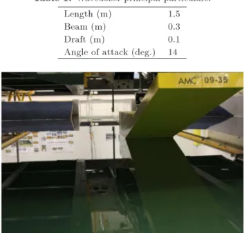
In order to generate waves, a moving wavedozer model was used as a pressure source during the experimental. The wavedozer model [19] was a wedge-shape model with constant beam (Figure 1). The main particulars of the wavedozer are listed in Table 1.

This model was tested in the Australian Maritime College towing tank, which had a length of 100 m and a width of 3.5 m. The water depth was 1.5 m in all conducted tests. Three wave probes were positioned at

Table 1. Wavedozer principal particulars.

Length (m) 1.5

Beam (m) 0.3

Draft (m) 0.1

Angle of attack (deg.) 14

Figure 1. Wavedozer model attached to the towing tank carriage.

Figure 2. Layout of probes with pressure source.

0.75, 1.0, and 1.25 m from the centre-line of the model to record the wave parameters (Figure 2), where y

was dened by the distance of the wave probe position over the width of the channel (y _{= y=W ). Two load}

cells were installed on the model to measure the vertical and drag forces. The model was tested at various depth Froude numbers from 0.43 to 0.99.

3. Numerical simulation

The CFD software ANSYS-Fluent version 14.5 was used as the ow solver [20]. The governing equations were three-dimensional Reynolds Averaged Navier-Stokes equations for incompressible ows. The Volume Of Fluid (VOF) approach was used with a time-dependent and explicit time discretization scheme em-ployed to solve the equations. The SIMPLE algorithm was used for the pressure-velocity coupling and the PRESTO scheme for the pressure interpolation. The k-epsilon model with the standard wall function was utilized for turbulence modelling. The 2nd order upwind scheme was used for solving the momentum

(3)

equations and the High Resolution Interface Capturing scheme (HRIC) for the solution to the volume fraction equations.

Figure 3 shows the computational grid domain. For the numerical investigation, a domain compris-ing 6 m in front of the model and 13.5 m behind it was considered. The heave and trim were xed at the same value as used in experimental tests. As the ow had a plane of symmetry about the centre plane, to decrease the processing time, half of the domain was used. The origin of the coordinate system was located at the middle of the model. The open channel boundary condition was used to specify the inlet and outlet boundary conditions. Inlet velocity and outow boundary conditions were selected for inlet and outlet boundaries, respectively. A symmetry plane was used along the centre plane, and the remaining boundary surfaces along the exterior of the domain were set to no-slip wall conditions. More details about mesh domain and cells' properties are presented in [21].

4. Validating the numerical approach

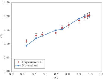
The results of the numerical simulation have been compared with experimental data in various gures. Figure 4 shows the drag coecient results for the

Figure 3. Computational grid domain.

Figure 4. Comparison of experimental and numerical drag coecients for dierent values of Frhat 1500 mm

water depth.

Figure 5. Comparison of experimental and numerical lift coecients for dierent values of Frhat 1500 mm water

depth.

experimental and numerical investigations, and Fig-ure 5 presents the vertical force (or lift) coecient for dierent speeds. Drag and vertical force coecients are dened as:

Cd =_{0:5 V}Drag₂_{D B} ;

Cl= _{0:5 V}Vertical force₂_{LWL B} ; (1)

where is water density, V is speed of the pressure source, D is draught, B is beam, and LWL is length of waterline. It should be mentioned that the water separates from model sides during tests and only model bottom remains wet [21]. In addition, the highest portion of total drag (95%) can be attributed to pressure drag [21]. Therefore, in Eq. (1), the area is equal to D B and in Eq. (2), the area is equal to LWL B. The standard error bars (5%) are shown for all the experimental data.

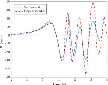
It is clear that the simulation results are in good agreement with the experimental data with respect to the forces. The percentage variations between numerical results and the experimental data are mostly less than 5%. To increase the accuracy of the results for lower speeds, the mesh should be rened; however, in this study, the higher speeds are of more interest. The free-surface elevation for depth Froude numbers 0.7 and 0.99 for nearest, middle, and farthest wave probes are presented in Figures 6 to 9. Free-surface elevations show that the Fluent software is able to predict the wave patterns at dierent lateral distances. The nu-merical method is validated by the presented results and it can be used to investigate the eects of changes in parameters. It should be mentioned that the rst wave behind the pressure source was considered as surfable wave; therefore, surface elevation of the rst

(4)

Figure 6. Free-surface elevation for Frh= 0:7 at 750 mm

lateral distance from centre-line (WP1).

Figure 7. Free-surface elevation for Frh= 0:99 at

750 mm lateral distance from centre-line (WP1).

wave behind the pressure source was considered and as soon as the rst wave reached steady state, the simulations were stopped. To improve the accuracy of the results in far led, the simulation time should be increased and mesh should be rened; however, in this study, this was unnecessary.

5. Investigating the eect of various parameters

5.1. Pressure source parameters

Draught, beam, and angle of attack were the main parameters of the wavedozer numerically investigated with respect to the height and propagation of the wave generated. Changing any of these parameters would alter the wavedozer's displacement. In this study, only one of the parameters was changed at a time and the rest were kept constant in order to compare the numerical results and examine the eect of the changed parameter.

5.2. Draught

Table 2 shows the dimensions of two wavedozers. Model 1 is the model which was used in the experi-mental tests and the previous simulations. To consider the eect of draught on generated waves, a new model (Model 2) was simulated. The draught of Model 2 was 20% more than that of Model 1. These simulations were conducted in deep water condition (1.5 m water depth). Since the tests were conducted in 1.5 m water depth, the draught change did not have a signicant inuence on the blockage factor. Blockage factor can be dened as:

Blockage factor ()

=_{Channel cross section area (A}Model cross section area (As)

c): (2)

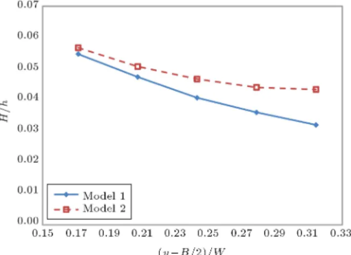
The comparison between Model 1 and Model 2 shows that increasing the draught causes increase in wave height. It is predicted that at a certain draught, the wave starts to break and further draught increases do not have eect on the height of the generated wave. Figures 10 to 13 present the comparison of wave heights

(5)

Table 2. Wavedozers dimensions. Draught

(m)

Beam (m)

Angle of attack (deg)

LWL (m)

Displacement (m3₎

Blockage factor

Model 1 0.1 0.3 14 0.40 0.006015 0.0057

Model 2 0.12 0.3 14 0.48 0.00866 0.0068

Figure 10. Non-dimensional wave heights variation with respect to lateral distances for Models 1 and 2 at

Frh= 0:75.

Frh= 0:9.

for two dierent models at dierent lateral distances, where y is lateral distance, B and W are model and channel widths, respectively, H is wave height of the rst wave behind the pressure source, and h is water depth.

5.3. Angle of attack

Another potentially important parameter is the angle of attack. The angle of attack is the angle between the entry surface and the water surface. The previous studies were conducted with a wavedozer with a 14-degree angle of attack. The 14-14-degree angle of attack was presented as the optimum angle in [19]. In this

Frh= 0:95.

Frh= 0:99.

study, wavedozers with dierent angles of attack were simulated. By altering the angle of attack, the Length of Waterline (LWL) and the displacement changed, and the draught and beam remained constant. The wavedozer with the lowest angle of attack had the largest displacement and vice versa.

Table 3 presents the wavedozers' parameters. Figures 14 to 17 illustrate the wave heights for dierent wavedozers at dierent values of Frh.

By decreasing the angle of attack, the variation of wave height with lateral distances decreased. For example, in Model 5 (angle of attack of 4 degrees), at

(6)

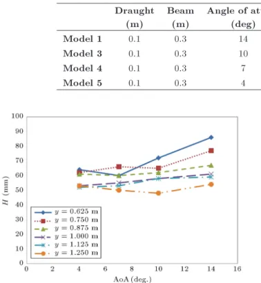
Table 3. Wavedozers with dierent angles of attack parameters. Draught

(m)

Beam (m)

LWL (m)

Displacement (m3₎

Blockage factor

Model 1 0.1 0.3 14 0.401 0.006015 0.0057

Model 3 0.1 0.3 10 0.567 0.008505 0.0057

Model 4 0.1 0.3 7 0.814 0.01221 0.0057

Model 5 0.1 0.3 4 1.43 0.02145 0.0057

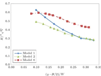
Figure 14. Variation of the height of the generated wave with respect to Angle of Attack (AoA) at dierent lateral distances for Frh= 0:75.

Frh= 0:9, the wave height was almost constant on the

entire width of the channel. By increasing the angle of attack, the maximum wave height increased due to increase in the pressure gradient. It can be said that

D

LWLpx, where px is pressure gradient in longitudinal

direction (p is pressure force). Therefore, by increasing the angle of attack in constant draught (D), the length of waterline (LWL) will decrease. Therefore, the pressure gradient will increase and, as a consequence, the height of the generated wave will increase. Model 5

has the largest displacement while it generates the lowest wave height. Increasing the displacement by changing the angle of attack (or LWL) has the opposite eect on wave height. By decreasing the angle of attack, the model drag decreases. Figures 18 and 19 show the drag and vertical forces for dierent angles of attack. The highest portion of total drag can be attributed to pressure drag [21]. Increasing the angle of attack increases the pressure drag and decreasing it increases the wetted area and, as a result, increases

(7)

Figure 18. The drag coecients variation with respect to angle of attack at dierent values of Frh.

Figure 19. The lift coecients variation with respect to angle of attack at dierent values of Frh.

the viscous drag. It can be concluded that Model 5 with the largest displacement generates the lowest wave height because it has minimum pressure drag, and Model 1 with the lowest displacement generates the highest wave height because it has maximum drag. 5.4. Beam

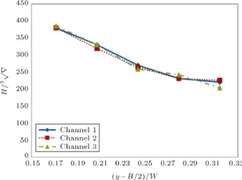
The eect of pressure source beam on the height and quality of the generated wave was investigated. For this investigation, the wavedozer beam was increased from 300 mm (Model 1) to 433 mm (Model 6). In addition, it should be noted that the wavedozer with 433 mm beam (Model 6) had the same displacement as

Figure 20. Non-dimensional wave heights variation with respect to lateral distances for Models 1, 2, and 6 at Frh= 0:75.

the model with 120 mm draught (Model 2), which had previously been used for draught investigation.

Table 4 presents the characteristics of these mod-els. By comparing Models 1 and 6, it is possible to see the eect of beam and displacement change on wave height and comparing Models 2 and 6 makes it possible to see the eect of altering beam and draught but maintaining displacement. The simulations were conducted in a channel with 3.5 m width and 1.5 m depth. Figures 20 to 23 illustrate the results for the aforementioned models at dierent values of Frh.

Table 4. The characteristics of pressure sources. Draught

(m)

Beam (m)

LWL (m)

Displacement (m3₎

Blockage factor

Model 1 0.1 0.3 0.40 0.120 14 0.006

Model 2 0.12 0.3 0.48 0.144 14 0.00866

(8)

The results show that by increasing the model beam, the generated wave height increases for all investigated values of Frh. The wave height of Model 6,

which has greater beam (the width of Model 6 is about 44% larger than those of Models 1 and 2), is about 28% to 98% larger than wave heights of Models 1 and 2 at various lateral distances. Comparison between Models 1, 2, and 6 shows that adding displacement increases wave height; however, the increase by increas-ing draught is small, whereas the increase due to beam increase is large. The dierence between Models 6 and 2 can be explained by considering that the waterplane of Model 6 is larger than that of Model 2 (Table 4). Therefore, increasing the displacement by increasing the beam generates a higher wave than increasing the draught does. It is predicted that increasing the beam will increase the wave height until the wave starts to break and, then, further increase in beam does not have inuence on the wave height.

6. Pressure source prole shape

According to the study results of the angle of attack, it was seen that the waves generated by a model with 4-degree angle of attack had almost constant height across the channel, while the model with angle of attack of 14 degrees generated higher waves. However, the bow waves generated by the 4-degree angle of attack were larger than those by the 14-degree angle of attack. A new model (Model 8) was generated. This model had a constant beam with a 14-degree angle of attack at the front and a 4-degree angle of attack at the stern (Table 5). Figure 24 shows Model 8 schematically. Figures 25 to 28 show the results for Model 1 (14-degree angle of attack), Model 5 (4-degree angle of attack), and Model 8. The heights of the generated wave in

Table 5. The characteristics of Model 8.

Beam (m) 0.3

Length of water line (m) 0.4 Angle of attack in front (degree) 14 Angle of attack in stern (degree) 4.0

Draught (m) 0.1

Figure 24. Model 8 of B = 0.3 m, LWL = 0.4 m, AOA at transom = 4 degrees, AOA at front = 14 degrees, and D = 0:1 m.

(9)

Model 8 were smaller than those in Model 1, but the wave height decrease between the lateral distances of y_{= 0:57 and y}_{= 0:71 was slightly less than that in}

Model 1.

According to the results, it can be concluded that the angle of attack in the front of model (at the stagnation point) is more eective on the height of the generated wave, while the angle of attack at transom can have eect on wave quality. It means that the wave height decrease between lateral distances of 1.0 m and 1.25 m is slightly less than that in Model 1 and more than that in Model 8.

7. Channel parameters 7.1. Depth

The eect of water depth on generated wave height was investigated. Three water depths were considered and the wavedozer with 0.1 m draught and 0.3 m beam was simulated at 3 dierent speeds. The only dierence between channels was the water depth.

Table 6 presents Frh for the given speeds at

dierent water depths. Frh values at 1.66 m/s forward

speed for all 3 dierent depths were less than 1 (sub-critical Frh). Figure 29 shows the wave height results

at 1.66 m/s speed for the 3 dierent water depths. According to the results, the generated wave in the shallowest water had the largest wave height, because it had the highest Frh.

Table 6. Frhfor dierent speeds at dierent water depths.

h (m) V (m/s)

1.66 1.99 2.66 Channel 1 0.4 0.838 1 1.343 Channel 2 0.45 0.79 0.947 1.266 Channel 3 0.5 0.75 0.9 1.2

Figure 29. Non-dimensional wave heights variation with respect to lateral distances for 3 dierent water depths at 1.66 m/s speed.

(10)

Figure 30. Free-surface elevation at 0.75 m lateral distance and 1.99 m/s speed for 3 dierent water depths.

The Frhat 1.99 m/s speed and 0.4 m water depth

was equal to 1. The simulation results showed the generated bow wave (soliton wave) at this condition was larger than those in the two other conditions and the wave behind the pressure source had the lowest height at Frh= 10 (Figure 30). Figure 31 presents the

wave heights at dierent lateral distances for 3 dierent water depths at 1.99 m/s speed. Figure 32 presents the results for 2.66 m/s at dierent water depths. The Frh

for all 3 conditions is larger than 1. Figure 33 shows the time history of surface elevation at 0.75 lateral distance for 2.6 m/s speed at 3 dierent water depths. It can be seen that the shapes of the waves are the same for Frh larger than 1.2. It means the water depth does

not have inuence on the wave shape. Because the Frh

values are greater than one, the downstream pressure does not have eect on the up-stream.

Figure 33. Free-surface elevation at 0.75 m lateral distance and 2.66 m/s speed for 3 dierent water depths.

7.2. Blockage factor

By changing the water depth, depth Froude number and blockage factor will change simultaneously. It was shown in the previous section that changing the water depth had an eect on the generated wave characteristics. To separate the eect of depth Froude number and blockage factor by changing the water depth, a new channel was modelled (Channel 4) and the results were compared with the results for the two other channels.

Table 7 presents the parameters of the 3 Channels

Table 7. The parameters of 3 dierent channels for blockage factor investigation.

Width (m)

Depth (m)

Blockage factor ()

Channel 1 3.5 0.4 0.0214

Channel 2 3.5 0.5 0.0171

(11)

Figure 34. Wave heights variation with respect to lateral distances for 3 dierent water depths at 1.66 m/s speed.

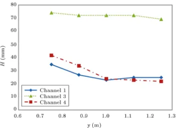
which were used in this comparison. Channels 1 and 4 had the same water depth, and Channels 3 and 4 had the same blockage factor but dierent water depths. The results for the 3 dierent speeds of 1.66, 1.99, and 2.66 m/s are presented in Figures 34 to 36.

The results indicate that the eect of depth Froude number on wave height is more important than that of the blockage factor for Frh < 1:0 and the

blockage factor in this range of Frhis negligible.

There-fore, higher Frh generates larger wave (Figure 34). In

Figure 35, the model in Channel 3 is in sub-critical (Frh = 0:9) and the models in Channels 1 and 4

are in critical (Frh = 1:0) Froude depth values. At

supercritical Froude depth values, the channel with the lowest blockage factor generates the highest wave (Figure 36). More investigations are required to nd the highest ineective blockage factor. At the highest ineective blockage factor, the channel's cross section would be the smallest, which does not have inuence on the parameters of the generated wave.

8. Concluding remarks

In this study, the inuences of pressure source param-eters, depth, and blockage factors were investigated. Draught, angle of attack, beam, and prole shape were investigated as the eective parameters of pressure source on wave height. Since the rst wave behind the pressure source was considered as surfable wave, the eect of parameters on this wave was investigated.

The investigation indicated that increasing draught, angle of attack, and beam would increase the height of the generated wave, while it was shown that wave height variation across the channel for a lower angle of attack was less than others. The pressure gradient would increase by increasing the angle of attack. Hence, the wave generated by the wavedozer of higher angle of attack was larger than that generated by the wavedozer of lower angle of attack. Comparing the results for the 2 dierent wavedozers with the same displacements and angles of attack, but dierent beams and draughts, showed that the model with the wider beam generated a higher wave. This means that the eect of beam on generated waves was greater than the eect of draught. The model with larger beam had larger water plane, which means the volume of displacement close to free surface in the model with larger beam was bigger than that in the model with larger draught. Consequently, the wave generated by wider wavedozer was higher than the other one. Meanwhile, it was expected that there would be a limitation on eective draught and the draughts larger than that would not have eect on the height of the generated wave. Since only the portion of vessel displacement near to free surface has eect on the wave generated, increasing the beam would increase the wave height until the wave does not break.

The water depth study showed that by decreasing the water depth for a given speed, larger wave height would be generated as long as the Frh was subcritical.

(12)

When Frh = 1, the bow (soliton) wave generated was

higher than the wave behind the pressure source. It was also shown that water depth did not have eect on the wave height for Frh more than 1.2. It means that

for this range of Frh, the downstream did not have

inuence on upstream, because the pressure source moved faster than the wave.

The blockage factor was investigated. The results indicated that the eect of depth Froude number on wave height was more important than that of the blockage factor for subcritical Froude depth values and the blockage factor at this range was negligible. At supercritical Froude depth values, the channel with the lowest blockage factor generated the highest wave. Further simulations are needed to nd the highest ineective blockage factor.

Acknowledgement

The authors thank the Australian Research Council (ARC), University of Tasmania, and Liquid Time Pty Ltd., who funded this research. This research was supported under the ARC Linkage Projects funding scheme (Project LP0990307).

Nomenclature

r Volume displacement Blockage factor Longitudinal distance Ac Channel cross section area

AOA Angle Of Attack

As Model cross section area

B Model beam Cd Drag coecient

Cl Lift coecient

D Model draught Frh Depth Froude number

H Wave height h Water depth LWL Length of waterline p Pressure

V Speed of model W Width of channel WP Wave probe y Lateral distance

y _y=W

Water density

References

1. Georgiadis, C. \Modeling boat wake loading on long oating structures", Computers & Structures, 18(4), p. 6 (1984).

2. Dam, K.T., Tanimoto, K., Nguyen, B.T., and Ak-agawa, Y. \Numerical study of propagation of ship waves on a sloping coast", Ocean Engineering, 33, p. 15 (2006).

3. Jiankang, W., Lee, T.S., and Shu, C. \Numerical study of wave interaction generated by two ships moving parallely in shallow water", Computer Methods in Applied Mechanics and Engineering, 190, p. 12 (2001). 4. Nanson, G., Krusenstierna, A.V., Bryant, E., and Renilson, M. \Experimental measurements of river bank erosion caused by boat-Generated waves on the Gordon River, Tasmania", Regulated Rivers, Research and Management, 9, p. 14 (1994).

5. Renilson, M.R. and Lenz, S. \An investigation into the eect of hull form on the wake wave generated by low speed vessels", 22nd American Towing Tank Conference, p. 6 (1989).

6. Robbins, A., Thomas, G., Renilson, M., and Macfar-lane, G. \Subcritical wave wake unsteadiness", RINA Transactions, International Journal of Maritime En-gineering, 153, Part A3 (2011).

7. Zibell, H.G. and Grollius, W. \Fast vessels on inland waterways", in The RINA International Conference on Coastal Ships and Inland Waterways, London, England (1999).

8. Macfarlane, G.J. and Bose, N. Wave Wake: Fo-cus on Vessel Operations Within Sheltered Aterways, SNAME, 006 (2012).

9. Koushan, K., Werenskiold, P., and Zhao, R. \Experi-mental and theoretical investigation of wake wash", in FAST, Southampton, UK, pp. 165-179 (2001). 10. Chandraprabha, S. and Molland, A.F. \A numerical

prediction of ash wave and wave resistance of high speed displacement ships in deep and shallow water", in Conference of Mechanical Engineering Network of Thailand, Khon Kaen, Thailand (2004).

11. Fontaine, E. and Tulin, M.P. \On the prediction of nonlinear free-surface ows past slender hulls using 2D+T theory: The evolution of an idea", in Fluid Dynamics of Vehicles Operating Near or in The Air-Sea Interface, Amsterdam, Netherland (1998). 12. Henn, R., Sharma, S.D., and Jiang, T. \Inuence of

canal topography on ship waves in shallow water", in 16th International Workshop on Water Waves and Floating Bodies, Hiroshima, Japan (2001).

13. Yang, Q., Faltinsen, O.M., and Zhao, R. \Wash of ships in nite water depth", in FAST, Southhampton, UK, pp. 181-196 (2001).

(13)

14. Raven, H.C. \Numerical wash prediction using a free-surface panel code", in International Conference on Hydrodynamics of High-Speed Craft-Wake Wash and Motion Control, London, UK (2000).

15. Kofoed-Hansen, H., Jensen, T., and Srensen, O.R. \Wake wash risk assessment of high-speed ferry routes - A case study and suggestions for model improve-ments", in International Conference on Hydrodynam-ics of High-Speed Craft-Wake Wash and Motion Con-trol, London, UK (2000).

16. Kim, Y. \Articial damping in water wave problems II: Application to wave absorption", International Journal of Oshore and Polar Engineering, 13, p. 5 (2003).

17. Javanmardi, M., Binns, J., Renilson, M.R., Thomas, G., and Huijsmans, R. \The formation of surfable waves in a circular wave pool- comparison of numerical and experimental approaches", in 31th International Conference on Ocean, Oshore and Arctic Engineer-ing, Rio de Janeiro, Brazil (2012).

18. Javanmardi, M., Binns, J., Thomas, G., and Renilson, M.R. \Prediction of water wave propagation using computational uid dynamics", in 32th International Conference on Ocean, Oshore and Arctic Engineer-ing, Nantes, France (2013).

19. Driscoll, A. and Renilson, M.R. \The wavedozer. A system of generating stationary waves in a circulating water channel", AMTE(H) TM80013 (1980).

20. \ANSYS FLUENT User's Guid", ANSYS, Inc. (2011). 21. Javanmardi, M. \The investigation of high quality surng waves generated by a moving pressure source", PhD Thesis, University of Tasmania (2015).

Biographies

Mohammadreza Javanmardi is Adjunct Assistant Professor at Sharif University of Technology. His research focuses on the ship hydrodynamics, maneu-vering, wave, computational uid dynamics, and ex-perimental tests.

Jonathan Binns is Associate Research dean in the Australian Maritime College and the director of the ARC Research Training Centre for Naval Design and Manufacturing, University of Tasmania. He has trained and worked as a design and research engineer specialising in analysis of uid mechanics by theoretical and experimental means. His primary expertise is in a variety of model and full-scale experiments as well as potential ow and nite volume ow predictions. He has experience in hydrodynamic and structural design, research, development, and simulation of marine craft. Giles Thomas is BMT Chair of Maritime Engineering in University College London's Department of Mechan-ical Engineering. As a naval architect, his research focuses on the performance of ships, boats, and oshore structures. His specic interests include uid-structure interaction, hydrodynamics, full-scale measurements, model testing, and design. He is a fellow of the Royal Institution of Naval Architects (RINA) and a chartered engineer (CEng- Engineering Council of Great Britain). Martin Renilson is an Adjunct Professor in Hydro-dynamics at the University of Tasmania. His previous experiences include technical management and deputy general management of the Maritime Platforms and Equipment Group at QinetiQ.