Estimating the Parameters of Mixed Shifted Negative Binomial Distributions via an EM Algorithm

Sharif University of Technology

Transactions E: Industrial Engineering http://scientiairanica.sharif.edu

Estimating the parameters of mixed shifted negative

binomial distributions via an EM algorithm

M. Varmazyar

_{, R. Akhavan-Tabatabaei}

_{, N. Salmasi}

_{, and M. Modarres}

Received 24 September 2017; received in revised form 12 November 2017; accepted 2 January 2018

KEYWORDS Parameter estimation; Discrete Phase-Type (DPH) distributions; Expectation-Maximization (EM) algorithm;

Mixed shifted negative binomial distributions.

Abstract.Discrete Phase-Type (DPH) distributions have one property that is not shared by Continuous Phase-Type (CPH) distributions, i.e., representing a deterministic value as a DPH random variable. This property distinguishes the application of DPH in stochastic modeling of real-life problems, such as stochastic scheduling, in which service time random variables should be compared with a deadline that is usually a constant value. In this paper, we consider a restricted class of DPH distributions, called Mixed Shifted Negative Binomial (MSNB), and show its exibility in producing a wide range of variances as well as its adequacy in tting fat-tailed distributions. These properties render MSNB applicable to represent data on certain types of service time. Therefore, we adapt an Expectation-Maximization (EM) algorithm to estimate the parameters of MSNB distributions that accurately t trace data. To present the applicability of the proposed algorithm, we use it to t real operating room times and a set of benchmark traces generated from continuous distributions as case studies. Finally, we illustrate the eciency of the proposed algorithm by comparing its results with those of two existing algorithms in the literature. We conclude that our proposed algorithm outperforms other DPH algorithms in tting trace data and distributions.

© 2019 Sharif University of Technology. All rights reserved.

1. Introduction

Phase-type (PH) distributions, introduced by Neuts [1,2], are a family of discrete and continuous probability distributions constructed by mixtures of geometric or exponential phases. Special properties and characteristics of PH distributions make them attractive for approximating a variety of random variables and modeling real-world stochastic arrival or

*. Corresponding author. Tel.: +98 21 6616 5719; Fax: +98 21 66022702

E-mail addresses: [email protected] (M. Varmazyar); [email protected] (R.

Akhavan-Tabatabaei); [email protected] (N. Salmasi); [email protected] (M. Modarres)

doi: 10.24200/sci.2018.5130.1117

service times [3]. The common property to Discrete PH (DPH) and Continuous PH (CPH) distributions is that the convolution, minimum, maximum, and convex mixtures of PH random variables yield new PH random variables. However, representing deterministic values by a PH random variable (deterministic values property) is restricted to the DPH distributions [2].

With regards to the property of deterministic values, shifting (adding a constant to) the DPH random variables results in a new DPH structure [2]. Using this property, we can derive the distribution function of the convolution or maximum/minimum of the DPH random variables with constant values. One important application of this derivation is in stochastic scheduling problems. In such problems, random processing times should be combined with constant durations (e.g., set up times) or the maximum/minimum of random times

should be compared with constant deadline values in order to compute the objective function.

Shifted Negative Binomial (SNB) distribution is a subclass of DPH distributions and the discrete anal-ogous to the Erlang distribution in the CPH class. The Mixed Shifted Negative Binomial (MSNB) distribution is a mixture of independent SNB distributions and a subclass of DPH. The MSNB family is the discrete equivalent of Hyper-Erlang Distribution (HErD) in the CPH family. Similar to the HErD, which can approx-imate any distribution on R [4,5], the MSNB subclass models distributions that are dened on N. Moreover, the Coecient of Variation (CoV) of MSNB distribu-tion can be tuned to less than, equal to, or greater than unity. Also, it provides good approximations to fat-tailed distributions. These properties render MSNB desirable for tting data on high variance service times or when the tail of service time distribution is heavier than the exponential distribution [6]. Therefore, in this research, our goal is to estimate the parameters of the MSNB distribution in order to t empirical service time data with such characteristics.

In the previous research, some approaches to tting the parameters of a general DPH distribution have been provided. Horvath and Telek [7] presented a tool called Pht, which estimated the parameters of Acyclic DPH (ADPH) and Acyclic CPH (ACP) distributions to minimize a distance measure by using a non-linear optimization method. The purpose of their algorithm was optimization by iterative linearization to numerically compute the partial derivatives.

The rst detailed study on DPH and ADPH distributions and their tting methods by Maximum Likelihood (ML) estimation was conducted by Bobbio et al. [8]. They also proved several properties of ADPH distributions and showed that the ADPH distribu-tions had a unique minimal representation, named the canonical form.

Callut and Dupont [9] studied the Expectation-Maximization (EM) algorithm to t the general DPH distributions. Their algorithm was an adapted version of the EM algorithm proposed by Asmussen et al. [10], which applied to continuous PH distributions. Three dierent methods, namely an EM algorithm, a Gibbs sampler algorithm, and a Quasi-Newton method, were applied for maximum likelihood estimation of general DPH distributions by Bladt et al. [11].

New results on the canonical representation of DPH with 2 and 3 phases (DPH (2) and DPH (3)) as well as Discrete Markov Arrival Processes (DMAP) with 2 phases (DMAP (2)) were presented by Meszaros et al. [12]. They presented explicit formulae to match parameters applying canonical forms (DPH (2), DPH (3), and DMAP (2)) and gave moments and corre-lation bounds. They showed the eciency of tting procedures with numerical examples. The Canonical

Representation of DPH (CRDPH) distributions with 3 phases (CRDPH (3)) was investigated by Horvath et al. [13]. They demonstrated that the problem of CRDPH (3) was far more complicated than the one of CPH distribution with 3 phases. They also needed to dene 8 dierent subclasses of DPH distribution with 3 phases for their canonical representation.

In this research, we present an EM algorithm to estimate the parameters of MSNB distributions. The advantages of the EM algorithm over other alternatives such as non-linear programming have been explored by Springer and Urban [14]. The most signicant property of the EM algorithm is guaranteeing the increase in the likelihood at each iteration. The other reason is that the EM algorithm needs neither the analytic expression nor the gradient of the log-likelihood function, and it does not even require being dierentiable. It also estimates the parameters of the distribution from a given data trace when the data has some missing values or is incomplete. The time complexity of the EM algorithm is linear, only depending on the number of SNB branches, and independent of the number of states. The number of SNB branches might be remark-ably lower than the number of states in most cases. Therefore, the tting algorithm by EM algorithm is rather stable because of the specic structure of the ADPH distribution, which provides a reliable and fast convergence of the EM algorithm.

In Section 2, we dene the MSNB distribution by PH representation and prove some of its properties for approximating fat-tailed trace data. In Section 3, we propose a specialized EM algorithm to t the parameters of the MSNB distribution and use this modied EM algorithm to t continuous distributions. In Section 4, we showcase the applicability of the proposed algorithm to t real-world operating room service time data as well as a set of benchmark traces generated from conventional distributions. We compare the accuracy of our results with two other algorithms designed by Thummler et al. [4] and Bladt et al. [11]. In Section 5, we provide the conclusions and show directions for future research.

2. Mixed shifted negative binomial distribution and its properties

The DPH distributions are constructed by a system of one or a group of inter-related geometric distributions occurring in sequence or phases (see Appendix A for detailed description and properties).

Shifted Geometric (SG) distribution is another nonequivalent denition of the geometric distribution, which describes the number of failures before the rst success (as opposed to the number of trials until suc-cess) in an innite sequence of independent Bernoulli trials. Shifted Negative Binomial (SNB) distribution is

the convolution of a number of SG random variables, dened as the number of failures before reaching a xed number of successes in a sequence of Bernoulli trials. In Appendix B, we present the denition and properties of SG and SNB distributions in PH representation. In the rest of this section, we present the denition and properties of the Mixed Shifted Negative Binomial (MSNB) distribution.

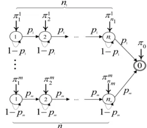
A mixed shifted negative binomial distribution (X MSNB(m; ni; pi; i)) is considered as a

mix-ture of m mutually independent SNB random vari-ables, weighted by the probability vector = [1; 2; ; m], in which i 0 and the vector is

stochastic, i.e.,Pm_i=1i= 1. Let nidene the number

of phases of the ith SNB distribution. Then, the MSNB probability mass function is given by Eq. (1) [29]:

Pr(X = x) =Xm

i=1

i

x + ni 1

ni 1

(1 pi)xpnii;

for x = 0; 1; (1)

The state space includes one absorbing state and P_m

i=1ni transient states. The DPH representation of

the MSNB distribution can be described by Eq. (2) and is illustrated in Figure 1.

MSNB= (MSNB1; MSNB2; ; MSNBm);

MSNBi = 1i; i2; ; ini

; i

j = i

ni

j 1

(1 pi)ni (j 1)pj 1i ;

for j = 1; ; ni; i = 1; ; m;

TMNB=

0 B B B @

T1 0 0

0 T2 0

... ... ... 0 0 0 Tm

1 C C C

A; (2)

where Ti is a matrix shown in Eq. (3):

Ti=

0 B B B B B @

1 pi pi 0 0 0

0 1 pi pi 0 0

...

0 0 0 1 pi pi

0 0 0 0 1 pi

1 C C C C C A;

i = 1; ; m: (3)

The kth factorial moment of the MSNB distribution is calculated by Eq. (4):

Figure 1. The DPH representation of MSNB (m; ni; pi; i).

fk = E[X(X 1) (X k + 1)]

=Xm

i=1

i (n_(ni+ k) i)

(1 pi)k

pk i ;

for k = 1; 2; : (4)

Let H be a set of all MSNB distributions with n states, i.e.:

H = (

Pr(X) : Pr(X = x) =Xm

i=1

i

x + ni 1

ni 1

(1 pi)xpnii;

x = 0; 1; ; Xm

i=1

i= 1; m

X

i=1

ni= n

) : (5) Note that set H contains all MSNB distributions including at most n states and the MSNB with less than n states can be acquired by setting some ivalues

to zero. We present the following theorem to show the versatility of the MSNB in approximating general distributions on N.

Theorem 1. The set H has the following properties:

1. Let F denote the set of all discrete distributions with nite support on N. Then, H is a dense set in F, i.e., any distribution on N can be approximated by MSNB distribution;

2. Let h denote an MSNB distribution and be out of the set H, with n 2. The parameters of h (MSNB distribution) can be tuned such that the Coecient of Variation (CoV) takes an arbitrary value less

than, equal to, or greater than unity. It can also be tuned such that its CoV takes value as large as or as small as desired.

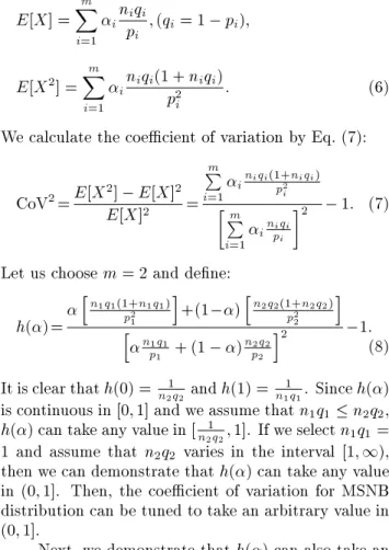
Proof. (1) is proven by weak convergence rule as shown by Verbelen [15]. We concentrate on the proof of (2). The rst and the second moments of MSNB distribution are given by Eqs. (1) and (4):

E[X] =Xm

i=1

in_piqi

i ; (qi= 1 pi);

E[X2_{] =}Xm i=1

iniqi(1 + n_p2 iqi)

i : (6)

We calculate the coecient of variation by Eq. (7): CoV2=E[X2_E[X]] E[X]₂ 2=

m

P

i=1i

niqi(1+niqi)

p2 i

_Pm

i=1i niqi

pi

2 1: (7)

Let us choose m = 2 and dene: h()=

h

n1q1(1+n1q1)

p2 1

i

+(1 )hn2q2(1+n2q2)

p2 2

i h

n1q1

p1 + (1 )

n2q2

p2

i2 1:

(8) It is clear that h(0) = 1

n2q2 and h(1) =

1

n1q1. Since h()

is continuous in [0; 1] and we assume that n1q1 n2q2,

h() can take any value in [ 1

n2q2; 1]. If we select n1q1=

1 and assume that n2q2 varies in the interval [1; 1),

then we can demonstrate that h() can take any value in (0; 1]. Then, the coecient of variation for MSNB distribution can be tuned to take an arbitrary value in (0; 1].

Next, we demonstrate that h() can also take an arbitrary value in [1; 1). We consider n1q1= n2q2= 1;

then:

g(; p1; p2) =

2h p2 1

i

+ 2h(1 )_p2 2

i h

p1 +

(1 ) p2

i₂ 1

= 2 + 2(1 ) h

p1

p2

i₂ h

+ (1 )p1

p2

i₂ 1;

! 2 1

p1

p2 ! 0

; (9)

from which we reach the conclusion that when we select and p1

p2 suciently small, g(; p1; p2) can take

value as large as desired. In addition, g(0:5; p; p) = 1. Since g(; p1; p2) is continuous in [0; 1] [0; 1] [0; 1],

g(; p1; p2) can take any value in [1; 1). Thus, the

coecient of variation can also be tuned to take value in [1; 1). This ends the proof of (2).

Notably, Theorem 1 states that any probability mass function with its domain in the natural numbers can be approximated arbitrarily closely by the proper selection of MSNB parameters. Then, for every point of a general probability mass function f 2 F, choosing a sequence of MSNB distributions with m SNB branches with each one having scale parameter, p, is possible.

Next, we show that the MSNB distribution can also approximate the fat-tailed distributions properly. Let F (x) be a cumulative MSNB distribution function given in Eq. (1), and F (x) = 1 F (x) be a complemen-tary cumulative MSNB distribution function calculated by:

F (x) =Xm

i=1 i 1 X k=x+1

k + ni 1

ni 1

(1 pi)kpnii: (10)

The distribution is called fat-tailed if Complementary Cumulative Distribution Function (CCDF) ( F (x)) is in the order of 1

xr, where x is suciently large for

r > 0. Intuitively, a fat-tailed distribution has a \fat tail" compared to the exponential distribution. Based on the denition of fat-tailed distribution, we study the property of F (x). In order to determine whether a distribution is a fat-tailed distribution, we observe the probability mass functions on the log-linear graphs. We consider MSNB distribution with MSNB (m = 4, ni = [2; 3; 4; 5], pi = [0:2; 0:3; 0:5; 0:7], and

i = [0:1; 0:2; 0:3; 0:4]) as an example and compare

it with the exponential distribution as illustrated in Figure 2. In fact, the MSNB distribution does provide the fat-tailed property in the time range of interest.

The innite variance is another specication of the fat-tailed distribution. We show that the MSNB

Figure 2. Comparing the fat-tailed property for MSNB and exponential distributions.

distributions can be tuned to take a nite bounded ex-pectation with a suciently large variance. In Eq. (6), we show that we can select i and pi appropriately;

then, E[x] is nite while E[x2_{] is suciently large. For}

example, when we select m = 2, r > 1, 1 = p1_r,

p1= p1_r, and p2= 1:

E[x] = n1

1 p1_r

< n1;

E[x2_{] = n} 1pr

1 p1

r 1 + n1

1 p1 r

n1pr ! 1 (r ! 1): (11)

In this section, we demonstrated the PH repre-sentation of MSNB distribution and its properties such as approximating any distribution on N, wide range of CoV, and fat-tailed property.

In the next section, we introduce an EM algorithm to estimate the parameters of the MSNB distribution by tting high variance or fat-tailed service time data.

3. An EM algorithm to t mixed shifted negative binomial distributions

The EM algorithm is an iterative approach to derive maximum likelihood for estimating the parameters of stochastic models, which are dependent on unobserved latent variables. Each iteration of EM algorithm consists of two steps: an expectation (E) step and a maximization (M) step. In the E step, a function is created for the expectation of the log-likelihood and evaluated using the current estimate of the parameters. In the M step, the parameters are computed while maximizing the expected log-likelihood determined in the E step. These estimated parameters are then applied to nd the distribution of the latent variables in the next E step.

In the rest of this section, we rst explain tting a mixture-density with the EM algorithm and present its application to the MSNB distributions. Then, we discuss the implementation of the EM algorithm over the weighted discrete sample to t continuous distributions by the MSNB distribution.

3.1. MSNB parameter estimation via an EM algorithm

One of the most common issues related to EM al-gorithm is the mixture-density parameter estimation method [16,17]. The probabilistic model of this method is assumed as follows:

Pr (x j) =Xm

i=1

iPri(x ji) ; (12)

where the parameters are = (1; ; m; 1; ;

m), in whichPm_i=1i= 1 and each Priis a probability

mass function parameterized by i. In other words,

m-component probability mass functions are mixed using m mixing coecients: i, i = 1; ; m. Generally,

i is a vector of parameters for each probability mass

function, Pri, while it is a single value in the proposed

EM algorithm.

Let X = fx1; ; xNg be an incomplete dataset

and Y = fyjgNj=1 be the existence of unobserved

data items, where the values inform which component function \generates" each data item of X . Therefore, assume that yj 2 f1; ; mg, for j = 1; ; N, and

yj = i if the jth sample (xj) is generated by the ith

mixture component. If the value of Y is known, the likelihood expression can be calculated by Eq. (13):

log L ( jX ; Y ) = log (Pr (X ; Y j)) =XN

j=1

log (Pr (xjjyj) Pr(y))

=

N

X

j=1

log yjPryj xjyj

: (13) The dilemma in dealing with Eq. (13) is that the values of yj are usually unknown. If yj is

consid-ered as random values drawn from a random variable Y, the derivation of expression for the probability mass function of unobserved data, shown by q(y), is possible. At rst, the parameters for probabil-ity mass function are guessed, i.e., the parameters ^ = (^1; ; ^m; ^1; ; ^m) are guessed as proper

parameters for likelihood L( ^jX ; Y). Given ^, the probability Pri(xjj^i) can be easily computed for each

i and j. Moreover, the mixing parameters, denoted by i, are considered as prior probabilities of each

mixture component or the probability of selecting the ith mixture component. Thus, the probability mass function of the unobserved data calculated by the observed data X and the estimates ^ are com-puted by applying Bayes's rule in Eqs. (14) and (15).

qyjxj; ^

=q

yj ^

Prxjyj^

Prxj ^

= ^yj:Pryj

xj^yj

m

P

i=1^i:Pri(xj

^i)

; (14)

qyX ; ^=YN

j=1

qyjjxj; ^

where y = fy1; ; yNg is a sample of the unobserved

data independently drawn from Y. The expectation value of the complete-data log-likelihood is given by Eq. (16) by considering the unknown random variable Y, the observed data X , and the current parameter estimates ^:

Q; ^=Ehlog L ( jX ; y ) jX ; ^i =X

y2 N

X

i=1

log (yipyi(xijyi))

N

Y

j=1

qyjjxj; ^

: (16) Integrating Eqs. (13) and (15) into Eq. (16) produces Eq. (17) according to Bilmes [18].

Q; ^=Xm

l=1 N

X

i=1

log(l):q

lxi; ^

+Xm

l=1 N

X

i=1

log (pl(xijl)) :q

lxi; ^

: (17) The computation of the expectation in Eq. (17) includes the E step of the EM algorithm. Generally, the main problem in calculating this expectation is to nd an expression for the distribution of the unobserved data, although the distribution of the unobserved data can be easily calculated by Eqs. (14) and (15). The purpose of M step in EM algorithm is to maximize the expectation determined in the E step by considering . To maximize Eq. (17), we can independently maximize the term including i

(rst sum in Eq. (17)) and the term including i

(second sum in Eq. (17)), because both terms are not relevant. According to Bilmes [15] and McLachlan and Krishnan [16], a Lagrange multiplier can be used to obtain the expression for i, resulting in:

i= _N1 N

X

j=1

qixj; ^

: (18)

In order to estimate the parameters of MSNB distributions, we apply the proposed EM algorithm. The ith mixture component of MSNB distributions is an SNB distribution with a xed number of phases shown in Eq. (19).

Pri(xjjpi) =

xj+ ni 1

ni 1

(1 pi)xjpnii: (19)

The mixture distribution is dened by the vector of . The parameters i and pi, i = 1; ; m, are

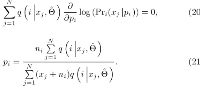
determined according to Eqs. (18) and (21). The value of pi can be calculated by Eq. (21) and integrating

Eq. (19) into Eq. (20) and applying logarithm-rules:

N

X

j=1

qixj; ^ @_@p

i log (Pri(xjjpi)) = 0; (20)

pi=

ni N

P

j=1q

ixj; ^

N

P

j=1(xj+ ni)q

ixj; ^

: (21)

Note that the value of piis always no more than one and

the condition of probability is satised by this equation. 3.1.1. Implementation and time complexity of the EM

algorithm

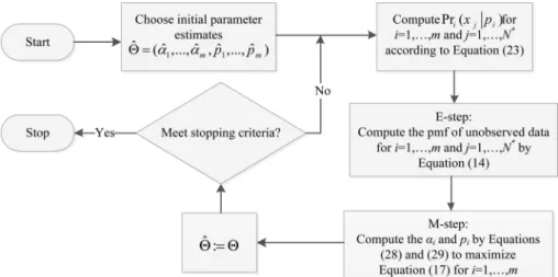
The EM algorithm starts with estimating the initial parameters = (1; ; m; p1; ; pm) and iterates

between the E step and the M step by using three Eqs. (14), (18), and (21) to reach the stopping crite-ria. The owchart of this algorithm is presented in Figure 3. Each iteration is guaranteed to increase the

log-likelihood value and the algorithm is guaranteed to converge to a local maximum of the likelihood func-tion [19]. To check whether convergence is achieved, the relative dierence of the log-likelihood values of successive iterations is computed and the algorithm stops when the computed dierence is less than a predened value of ", e.g., " = 10 6_.

By a given number of branches (m) and a number of phases of each branch (ni), the EM algorithm

determines the best setting of parameter vectors and p. However, in order to nd the \best" distri-bution, all MSNB distributions have to be considered as candidates. Thummler et al. [4] presented the dis-crete parameter setting for Hyper-Erlang Distribution (HErD) and used the recursive formula to consider all possible settings in an algorithmic fashion. In this paper, Thummler's recursive formula [4] is applied to nd the best MSNB distribution according to Eq. (22).

'i(n; j) = bn=ic_X

r=j

'i 1(n r; r);

where: '1(n; j) =

(

0; if j > n

1; if j n (22)

Direct computation of the SNB distribution (Eq. (19)) can reveal numerical diculties because large factorials must be computed for a high number of phases (e.g., n > 50). As a solution to this diculty, the logarithmic form is proposed and shown in Eq. (23):

Pri(xjjpi)

= eniln(pi)+xjln(1 pi)+ln(ni+xj 1)! ln(xj)! ln(ni 1)!:

(23) Also, the logarithms of the factorial values are com-puted by Eq. (24) before the EM algorithm starts:

ln r! =Xr

i=1

ln i: (24)

The time complexity of the proposed EM algorithm depends on its two main steps (E and M). The complexity of the E step is O(m:N) in computing the numerator and denominator of the unobserved data based on Eq. (14). The complexity of the M step is also O(m:N). The overall complexity of each iteration in the EM algorithm is O(m:N).

3.2. Fitting MSNB distributions to continuous distributions

In this section, we apply the proposed algorithm to t the data generated from continuous distributions. To approximate a continuous distribution by MSNB, a discretization method should be considered. The following steps are required to this end.

Step 1: Apply the discretization method and gener-ate discrete samples;

Step 2: Implement the EM algorithm by using MSNB over the discrete sample provided in Step 1. 3.2.1. Discretization method

Bobbio et al. [8] introduced a discretization method based on the Cumulative Distribution Function (CDF). In this method, nite (ordered) set S = fx1; x2; x3; g

(with x1 < x2 < x3 < ) is dened by multiplying

an integer with discretization interval (), i.e., xi= i.

Then, a probability mass is assigned to each element of S by Eq. (25):

wi= FX

xi+ xi+1

2

FX

xi 1+ xi

2

; i > 1 and w1= FX

x1+ x2

2

; (25) where FX(x) is the cdf of x and wi is the probability

associated with xi.

Dougherty et al. [20] proposed the \equal with interval binning" method for the case of using the generated traces instead of probability distribution function. It involves sorting the value bounded by xmin

and xmax, and dividing the range of values by k equally

sized bins by Eq. (26), in which k is a parameter given by the user:

=

xmax xmin

k

: (26)

The bin thresholds are computed by xmin+ i, where

i = 1; ; k. The probability mass (wi) is dened by

Eq. (27): wi= _Pkmi

j=1mj

; for i = 1; ; k: (27) In this equation, mi is the number of values that fall

into each of the bins.

3.2.2. Implementation of the EM algorithm over the weighted discrete sample

In Section 3.1, the proposed EM algorithm is based on the incomplete dataset, X = fx1; ; xNg, with weight

one. When the discretization method is considered as an approximation of continuous distributions, the incomplete dataset, X = fx1; ; xNg, with weight

one is substituted by incomplete dataset, X ₌

fx

1; ; xNg, with weight wi (Eq. (25) or (27)). The

modied set includes N_{elements with dierent values.}

Thus, Eqs. (18) and (21) can be eciently calculated by Eqs. (28) and (29), respectively:

i= _NP1

k=1wj

X

lim itsN

j=1wj:q

ixj; ^

Figure 4. Flowchart of the modied EM algorithm tailored to mixed shifted negative binomial distribution.

pi=

ni N

P

j=1wj:q

ix

j; ^

N

P

j=1wj:(x j+ ni):q

ix

j; ^

: (29)

The owchart of the modied EM algorithm is shown in Figure 4. Similar to the proposed algorithm in Section 3, the modied EM algorithm based on Eq. (22) determines the best setting of the parameter vectors and p by a given number of branches (m) and number of phases of each branch (ni). The computational

complexity of the E and M steps is O(m:N_{). Thus,}

the overall time complexity of one iteration for the EM algorithm is O(m:N_).

4. Results

In this section, we apply the proposed EM algorithm to t real-world operating room service times as well as six synthetically generated trace datasets from continuous distributions. The algorithm is coded in MATLAB 2014a [21] and performed on a personal computer with Intel(R) Core(TM) i3-2120, running at 3.30 GHz with 8 GB RAM.

4.1. Fitting MSNB distributions to real operating room data

To study an example with real data, the proposed EM algorithm is applied to t three dierent datasets of Start Anesthesia to Start Operation (SASO), Op-erating Room (OR), and Post-Anesthesia Care Unit (PACU) times. SASO time is dened as the duration of time from starting anesthesia procedure until starting the operation. OR time is the time of operation and PACU time is the recovery time of patients from anesthesia after the operation. The three datasets are collected from orthopedic operating theatre in the Scottish NHS hospital from 1998 to 1999, and are used in other studies [22].

Figure 5. Original dataset of SASO and the approximating distributions.

We compare the tting quality of the proposed EM algorithm (EM-MSNBD) with the quality of an EM algorithm designed for general DPH distributions (EM-DPH) presented by Bladt et al. [11] and the EM algorithm for the continuous HErD (EM-HErD) developed by Thummler et al. [4]. This algorithm is one of the best-performing algorithms in tting CPH [23]. The tting quality is measured by four dierent criteria, i.e., the rst three moments and the chi-square statistic (2₌ (trace data result of algorithm)2

trace data ).

The stopping criterion for all algorithms is convergence with " = 10 6_.

In Figures 5 to 7, the empirical distributions of SASO, OR, and PACU traces as well as the probability mass and density functions for the tted MSNB, general DPH, and HErD with 10 states are illustrated. The curve tting of MSNB shows that the proposed algorithm ts adequately to the fat-tailed data traces and conrms the fat-tailed property of MSNB distributions discussed in Section 2.

The results of tting quality are presented in Table 1. Relative errors of the rst three moments and the chi-square measure are represented in Table 2. According to Table 2, the relative errors of the rst

Table 1. Quality indices for tted MSNBD, DPH distribution, and HErD for three datasets.

Trace EM-MSNBD EM-DPH EM-HErD

SASO

First moment 19.75 19.75 19.75 19.75

Second moment 557.56 560.11 538.59 556.99

Third moment 22600.79 23487.23 19186.93 22935.57

CPU time (sec) 4.18 190.05 4.60

Number of phases 2,2,6 | 2,2,2,4

i 0.04; 0.34; 0.62 | 0.06; 0.04; 0.05; 0.85

pi or i 0.04; 0.10; 0.24 | 0.05; 0.10; 0.48; 0.21

OR

First moment 51.44 51.44 51.44 51.44

Second moment 4321.42 4372.55 4373.14 4331.21 Third moment 495266.84 515595.72 542221.03 497585.35

CPU time (sec) 2.81 1002.07 3.46

Number of phases 1,3,6 | 2,4,4

i 0.00; 0.57; 0.43 | 0.00;0.47;0.53

pi or i 0.33; 0.04; 0.21 | 1.48; 0.05; 0.16

PACU

First moment 9.49 9.49 9.49 9.49

Second moment 1559.53 1575.99 1946.51 1606.13 Third moment 684423.87 854044.08 1445876.41 893073.27

CPU time (sec) 2.12 378.70 2.29

Number of phases 1,3,6 | 1,2,3,4

i 0.02; 0.13; 0.85 | 0.02; 0.11; 0.75; 0.12

pi or i 0.00; 0.20; 0.57 | 0.00; 0.15; 0.58; 2.82

Figure 6. Original dataset of OR and the approximating distributions .

moment for all algorithms in each dataset are zero. The relative errors of the second and third moments and the chi-square measure for MSNBD and EM-HErD algorithms are nearly equal in all datasets, while these measures are relatively high for the EM-DPH algorithm. Therefore, we conclude that the tting quality of our proposed EM-MSNBD algorithm is as adequate as the tting quality of EM-HErD.

Figure 7. Original dataset of PACU and the approximating distributions.

A single-factor (algorithm eect) experiment with three levels (number of algorithms) is performed in order to statistically compare the performance of the three mentioned algorithms [24]. The hypothesis to be tested is as follows:

H0: EM-MSNBD = EM-DPH = EM-HErD;

Table 2. Relative errors of rst three moments and chi-square measure for three datasets.

EM-MSNBD EM-DPH EM-HErD

SASO

First moment 0.00% 0.00% 0.00%

Second moment 0.46% 3.40% 0.10%

Third moment 3.92% 15.11% 1.48%

Chi-square 0.08 0.20 0.08

OR

First moment 0.00% 0.00% 0.00%

Second moment 1.18% 1.19% 0.23%

Third moment 4.10% 9.48 % 0.46%

Chi-square 0.19 0.22 0.20

PACU

First moment 0.00% 0.00% 0.00%

Second moment 1.05% 24.81% 2.98%

Third moment 24.78% 111.25% 30.48%

Chi-square 0.65 0.63 0.65

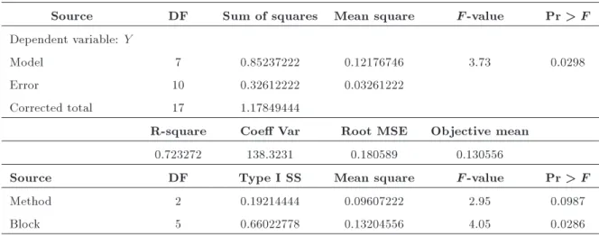
Table 3. The ANOVA table for real OR problem.

Source DF Sum of squares Mean square F -value Pr > F Dependent variable: Y

Model 7 0.85237222 0.12176746 3.73 0.0298

Error 10 0.32612222 0.03261222

Corrected total 17 1.17849444

R-square Coe Var Root MSE Objective mean

0.723272 138.3231 0.180589 0.130556

Source DF Type I SS Mean square F -value Pr > F

Method 2 0.19214444 0.09607222 2.95 0.0987

Block 5 0.66022778 0.13204556 4.05 0.0286

The single factor experiment is conducted as follows: Yab= + methoda+ blockb+ "ab; (31)

with the following characteristics:

Yab The response variable (relative errors);

The overall mean;

methoda The algorithm (eect factor),

a = 1; 2; 3;

blockb The second and third moments of each

dataset, b = 1; ; 6; "ab The error term.

The three algorithms are considered as the eect factor and the second and third moments of each dataset are considered as blocks. The experimental de-sign is coded in the Statistical Analysis System (SAS) software package, release 9.1 [25], with a signicance

level of 10%. The ANOVA tables are provided in Table 3. Based on the results of ANOVA, there is a statistically signicant dierence among the algorithms (the p-values are less than 0.1).

In order to nd the algorithm with the best performance, we also perform the Tukey test (Table 4). The results show that there is a signicant dierence among the EM-DPH and the two other algorithms, and the EM-MSNBD and EM-HErD algorithms are not statistically dierent. Throughout all experiments, the EM-MSNBD and EM-HErD algorithms outperform EM-DPH in terms of tting quality and CPU time requirements.

4.2. Fitting MSNB distributions to continuous distributions

Thummler et al. [4] generated six groups of samples by applying partial peak function of Weibull (1.0, 5.0), value function of uniform (0.5, 1.5), a

fat-Table 4. Tukey test for real OR problem; dierences of least squares means.

Algorithms comparison

Dierence between

means

90% Condence

limits

2-1 0.2183 [0.0294, 0.4073] *** 2-3 0.2200 [0.0310, 0.4090] *** 1-2 -0.2183 [-0.4073, -0.0294] *** 1-3 0.0017 [-0.1873, 0.1906] 3-2 -0.2200 [-0.4090, -0.0310] *** 3-1 -0.0017 [-0.1906, 0.1873]

_{1 is the EM-MSNBD algorithm; 2 is the EM-DPH algorithm;}

and 3 is the EM-HErD algorithm.

tailed distribution function of Weibull (1.0, 0.5), step function with shifted exponent, heavy-tailed distri-bution function of Pareto-II (1.5, 2.0), and multi-peak function with Matrix Exponential, which are all representative theoretical distributions. Each sample size is 104_{. The six groups of samples are chosen for}

the following reasons. Weibull distributions are often applied in the interpretation of experimental data in engineering such as reliability, queuing, transmission, etc. [26]. Uniform and shifted exponential distributions are dicult to closely approximate with a PH distri-bution [26]. Pareto-II distridistri-bution is an example of a heavy-tailed distribution, which is not monotonically decreasing [4]. The matrix exponential distribution has a matrix exponential representation, while it is not PH [26].

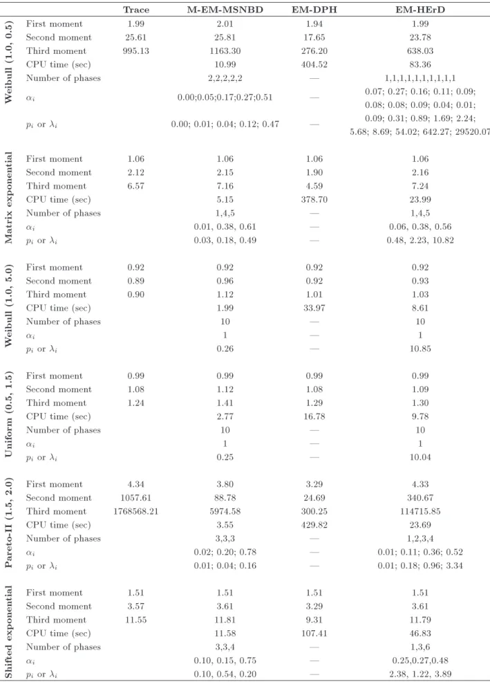
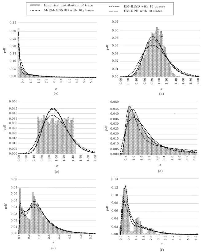
In this part, we test the three algorithms, namely the modied EM algorithm proposed in Section 3.2 (M-EM-MSNBD), the EM-DPH, and the EM-HErD, using the six groups of samples used by Thummler et al. [4]. The tting eects of the six groups of samples with three algorithms are illustrated in Figure 8 and the detailed records of tting quality measures are presented in Tables 5 and 6.

In order to compare our proposed algorithm with the two other algorithms, we draw conclusions based on Table 6 for each algorithm. The results of relative errors of the moments and the chi-square measure show that the M-EM-MSNBD algorithm can be considerably more ecient than the other two algorithms in tting the fat-tailed distributions such as Weibull (1.0, 0.5), as seen in Figure 8(a), and in the matrix exponential distributions, as shown in Figure 8(f). The results indicate that EM-DPH algorithm yields the lowest relative errors of moments and chi-square measure in symmetric distributions such as Weibull (1.0, 5.0) and uniform (0.5, 1.5) distributions as illustrated in Figure 8(b) and (c).

The results of EM-HErD algorithm show that the tting quality of the EM-HErD in Pareto-II (1.5, 2.0) and shifted exponent distributions (Figure 8(d) and (e)) is as good as the tting quality for EM-MSNBD. Based on six groups of samples, we rstly conclude that the results of relative errors of moments and the chi-square measure for the proposed algorithm and EM-HErD are nearly close to each other and dierent from the third one. Secondly, our proposed algorithm ts adequately to the fat-tailed distribu-tion.

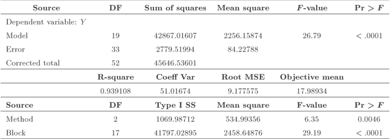
To statistically compare the performance of the three mentioned algorithms, we perform a single-factor (algorithm eect) experiment with three levels (number of algorithms), as in Section 4.1 and Eqs. (30) and (31). The rst, second, and third moments of each function are considered as blocks.

The experimental design is coded in SAS, release 9.1 [25], with a signicance level of 10%. The ANOVA tables and the results of Tukey test are provided in Tables 7 and 8. These results show that there is a signicant dierence among the EM-DPH and the two other algorithms, and the M-EM-MSNBD and EM-HErD algorithms are not statistically dierent. Throughout all experiments, M-MSNBD and EM-HErD algorithms perform better than EM-DPH in terms of CPU time requirement, as seen in Table 5. Also, in the majority of cases, M-EM-MSNBD and EM-HErD algorithms outperform EM-DPH in terms of tting quality, as seen in Table 6.

5. Conclusions and suggestions for future research

Discrete phase-type distributions have several advan-tages over their continuous equivalents. In this re-search, we considered the problem of tting a restricted class of DPH distributions, namely Mixed Shifted Neg-ative Binomial (MSNB) distributions, to trace data. We proved some properties of MSNB distribution to t trace data and developed a tting algorithm based on Expectation Maximization (EM) to estimate its parameters.

We measured the eectiveness of this algorithm by comparing it with two existing methods in the literature, HErD (for continuous data) and EM-DPH, using the operating room data and six bench-mark traces. To evaluate their goodness of t, we considered the rst three moments and the chi-square (2_{) measure and devised a single-factor (algorithm}

eect) experiment with three levels (number of algo-rithms).

The results of the experiment showed that (M-) EM-MSNBD and EM-HErD algorithms were not sta-tistically dierent, but they both outperformed the EM-DPH algorithm. Given that the EM-HErD

algo-Table 5. Quality indices for tted MSNBD, HErD, and DPH for synthetically generated traces.

Trace M-EM-MSNBD EM-DPH EM-HErD

W

eibull

(1.0,

0.5)

First moment 1.99 2.01 1.94 1.99

Second moment 25.61 25.81 17.65 23.78

Third moment 995.13 1163.30 276.20 638.03

CPU time (sec) 10.99 404.52 83.36

Number of phases 2,2,2,2,2 | 1,1,1,1,1,1,1,1,1,1

i 0.00;0.05;0.17;0.27;0.51 | 0.07; 0.27; 0.16; 0.11; 0.09;

0.08; 0.08; 0.09; 0.04; 0.01; pi or i 0.00; 0.01; 0.04; 0.12; 0.47 | 0.09; 0.31; 0.89; 1.69; 2.24;

5.68; 8.69; 54.02; 642.27; 29520.07

Matrix

exp

onen

tial First moment 1.06 1.06 1.06 1.06

Second moment 2.12 2.15 1.90 2.16

Third moment 6.57 7.16 4.59 7.24

CPU time (sec) 5.15 378.70 23.99

Number of phases 1,4,5 | 1,4,5

i 0.01, 0.38, 0.61 | 0.06, 0.38, 0.56

pi or i 0.03, 0.18, 0.49 | 0.48, 2.23, 10.82

W

eibull

(1.0,

5.0) First momentSecond moment 0.920.89 0.920.96 0.920.92 0.920.93

Third moment 0.90 1.12 1.01 1.03

CPU time (sec) 1.99 33.97 8.61

Number of phases 10 | 10

i 1 | 1

pi or i 0.26 | 10.85

Uniform

(0.5,

1.5) First moment_{Second moment} 0.99_1.08 0.99_1.12 0.99_1.08 0.99_1.09

Third moment 1.24 1.41 1.29 1.30

CPU time (sec) 2.77 16.78 9.78

Number of phases 10 | 10

i 1 | 1

pi or i 0.25 | 10.04

P

areto-I

I

(1.5,

2.0) First moment_{Second moment 1057.61}4.34 _88.783.80 _24.693.29 _340.674.33

Third moment 1768568.21 5974.58 300.25 114715.85

CPU time (sec) 3.55 429.82 23.69

Number of phases 3,3,3 | 1,2,3,4

i 0.02; 0.20; 0.78 | 0.01; 0.11; 0.36; 0.52

pi or i 0.01; 0.04; 0.16 | 0.01; 0.18; 0.96; 3.34

Shifted

exp

onen

tial First moment 1.51 1.51 1.51 1.51

Second moment 3.57 3.61 3.29 3.61

Third moment 11.55 11.81 9.31 11.79

CPU time (sec) 11.58 107.41 46.83

Number of phases 3,3,4 | 1,3,6

i 0.10, 0.15, 0.75 | 0.25,0.27,0.48

Table 6. Relative errors of the rst three moments and chi-square measure for synthetically generated Traces.

M-EM-MSNBD EM-DPH EM-HErD

W

eibull

(1.0,

0.5)

First moment 0. 91% 2.15% 0.00%

Second moment 0.79% 31.06% 7.12%

Third moment 16.89% 72.24% 35.88%

Chi-square 0.31 0.70 0.61

Matrix

exp

onen

tial First moment 0.00% 0.00% 0.00%

Second moment 1.39% 10.01% 1.93%

Third moment 8.91% 30.17% 10.20%

Chi-square 2.77 4.24 1.39

W

eibull

(1.0,

5.0)

First moment 0.00% 0.00% 0.00%

Second moment 8.02% 3.54% 4.55%

Third moment 24.96% 11.52% 14.43%

Chi-square 0.3 0.15 0.18

Uniform (0.5,

1.5)

First moment 0.00% 0.00% 0.00%

Second moment 4.49% 1.08% 1.40%

Third moment 14.09% 4.31% 5.18%

Chi-square 0.28 0.29 0.28

P

areto-I

I

(1.5,

2.0)

First moment 12.33% 24.11% 0.00%

Second moment 91.60% 97.66 67.78%

Third moment 99.66% 99.98% 93.51%

Chi-square 0.04 0.05 0.01

Shifted

exp

onen

tial First moment 0.11% 0.11% 0.00%

Second moment 0.92% 8.05% 0.76%

Third moment 2.18% 19.37% 2.07%

Chi-square 0.07 0.12 0.02

Table 7. The ANOVA table for continuous distributions.

Source DF Sum of squares Mean square F -value Pr > F Dependent variable: Y

Model 19 42867.01607 2256.15874 26.79 < :0001

Error 33 2779.51994 84.22788

Corrected total 52 45646.53601

R-square Coe Var Root MSE Objective mean

0.939108 51.01674 9.177575 17.98934

Source DF Type I SS Mean square F-value Pr > F

Method 2 1069.98712 534.99356 6.35 0.0046

Figure 8. Densities of tted MSNB, HErD, and DPH for synthetically generated traces: (a) Distribution of Weibull (1.0, 0.5), (b) distribution of Weibull (1.0, 5.0), (c) distribution of uniform (0.5, 1.5), (d) distribution of Pareto-II (1.5, 2.0), (e) distribution of shifted exponential, and (f) distribution of matrix exponential.

rithm is known as one of the most appropriate ones to t continuous PH distributions, we consider our proposed (M-)EM-MSNBD algorithm as equivalently appropriate to t discrete PH.

For further research, applying the result of the proposed EM algorithm in operating room scheduling

and developing a suitable method to solve this kind of problem are suggested.

Acknowledgment

Table 8. Tukey test for continuous distributions; dierences of least squares means.

Algorithms comparison

Dierence between

means

90% condence

limits

2-1 7.892 [1.483 14.301] *** 2-3 10.707 [4.298 17.116] *** 1-2 -7.892 [-14.301 -1.483] *** 1-3 2.815 [-3.502 9.132] 3-2 -10.707 [-17.116 -4.298] *** 3-1 -2.815 [-9.132 3.502]

_{1 is the M-EM-MSNBD algorithm; 2 is the EM-DPH}

algorithm; and 3 is the EM-HErD algorithm.

information of Scottish NHS Hospital from 1998 to 1999 by Professor John Bowers.

References

1. Neuts, M.F. \Computational uses of the method of phases in the theory of queues", Computers & Mathe-matics with Applications, 1(2), pp. 151-166 (1975).

2. Neuts, M.F., Matrix-Geometric Solutions in Stochastic Models: An Algorithmic Approach, Johns Hopkins University, Baltimore (1981).

3. Fackrell, M. \Modelling healthcare systems with phase-type distributions", Health Care Management Science, 12, pp. 11-26 (2009).

4. Thummler, A., Buchholz, P., and Telek, M. \A novel approach for phase-type tting with the EM algo-rithm", IEEE Transactions on Dependable and Secure Computing, 3(3), pp. 245-258 (2006).

5. Hu, L., Jiang, Y., Zhu, J., and Chen, Y. \Hybrid of the scatter search, improved adaptive genetic, and expectation maximization algorithms for phase-type distribution tting", Applied Mathematics and Com-putation, 219(10), pp. 5495-5515 (2013).

6. Anbazhagan, N., Stochastic Processes and Models in Operations Research, Hershey, Pennsylvania 701 E. Chocolate Avenue, Hershey, PA 17033, USA: IGI Global (2016).

7. Horvath, A. and Telek, M. \Pht: A general phase-type tting tool", Computer Performance Evaluation: Modelling Techniques and Tools, pp. 82-91 (2002).

8. Bobbio, A., Horvath, A., Scarpa, M., and Telek, M. \Acyclic discrete phase type distributions: properties and a parameter estimation algorithm", Performance Evaluation, 54(1), pp. 1-32 (2003).

9. Callut, J. and Dupont, P. \Sequence discrimination using phase-type distributions", Machine Learning: ECML 2006, pp. 78-89 (2006).

10. Asmussen, S., Nerman, O., and Olsson, M. \Fit-ting phase-type distributions via the EM algorithm", Scandinavian Journal of Statistics, 23(4), pp. 419-441 (1996).

11. Bladt, M., Esparza, L.J.R., Nielsen, B.F., et al. \Fisher information and statistical inference for phase-type distributions", Journal of Applied Probability, 48, pp. 277-293 (2011).

12. Meszaros, A., Papp, J., and Telek, M. \Fitting trac traces with discrete canonical phase type distributions and Markov arrival processes", International Journal of Applied Mathematics and Computer Science, 24(3), pp. 453-470 (2014).

13. Horvath, I., Papp, J., and Telek, M. \On the canonical representation of order 3 discrete phase type distri-butions", Electronic Notes in Theoretical Computer Science, 318, pp. 143-158 (2015).

14. Springer, T. and Urban, K. \Comparison of the EM algorithm and alternatives", Numerical Algorithms, 67(2), pp. 335-364 (2014).

15. Verbelen, R., Phase-Type Distributions & Mixtures of Erlangs, University of Leuven (2013).

16. O'Hagan, A., Murphy, T.B., and Gormley, I.C. \Com-putational aspects of tting mixture models via the expectation-maximization algorithm", Computational Statistics & Data Analysis, 56(12), pp. 3843-3864 (2012).

17. Xu, J. and Ma, J. \Fitting nite mixture models using iterative Monte Carlo classication", Communications in Statistics-Theory and Methods, 46(13), pp. 6684-6693 (2017).

18. Bilmes, J.A. \A gentle tutorial of the EM algo-rithm and its application to parameter estimation for Gaussian mixture and hidden Markov models", International Computer Science Institute, 4(510), p. 126 (1998).

19. McLachlan, G. and Krishnan, T., The EM Algorithm and Extensions, 382, John Wiley & Sons (2007).

20. Dougherty, J., Kohavi, R., and Sahami, M. \Super-vised and unsuper\Super-vised discretization of continuous feature", In Proceedings of 12th International Confer-ence of Machine Learning, pp. 194-202 (1995).

21. MATLAB Release 2014a, MathWorks, Inc. (2015).

22. Bowers, J. and Mould, G. \Managing uncertainty in orthopaedic trauma theatres", European Journal of Operational Research, 154(3), pp. 599-608 (2004).

23. Perez, J. and Riano, G. \Benchmarking of tting algorithms for continuous phase-type distributions", Working Paper, COPA Universidad de los Andes, pp. 1-20 (2007).

24. Chiarandini, M., Basso, D., and Stutzle, T. \Statistical methods for the comparison of stochastic optimizers", In MIC2005: The Sixth Metaheuristics International Conference, pp. 189-196 (2005).

25. SAS Release, 9.1, SAS Institute Inc. (2003).

26. Bobbio, A. and Telek, M. \A benchmark for PH esti-mation algorithms: results for Acyclic-PH", Stochastic Models, 10(3), pp. 661-677 (1994).

27. Latouche, G. and Ramaswami, V., Introduction to Matrix Analytic Methods in Stochastic Modeling, 5, Siam (1999).

28. Alfa, A., Applied Discrete-time Queues, Springer-Verlag New York (2016).

29. Varmazyar, M., Akhavan-Tabatabaei, R., Salmasi, N., and Modarres, M. \Classication and properties of acyclic discrete phase-type distributions based on ge-ometric and shifted gege-ometric distributions", Journal of Industrial Engineering International (Nov 2018).

Appendix A. Discrete phase-type distribution and its properties

Denition and notation

DPH distributions have been introduced and formal-ized by Neuts [1,2], as the distribution of time until absorption in a discrete-state Discrete-Time Markov Chain (DTMC) with n transient states and one ab-sorbing state. More precisely, assume that fX(n)gn0

denotes the DTMC with nite state space S = f0; 1; 2; ; ng, where the absorbing state is numbered 0 and the transient states are numbered 1; 2; ; n. DPH distribution is dened by Z = inf(i 2 N : Xi = 0) with representation (; T) and is shown by

Z PHd(; T). The one-step transition probability

matrix of the corresponding DTMC can be partitioned as:

P =

T t 0 1

; (A.1)

where T is a square matrix of dimension n, t is a column vector, and 0 is a row vector of dimension n. Since P is a transition probability matrix, we have Tij 0, ti 0 8i, j 2 S, and T1 + t = 1, where 1 is

the column vector of 1s of the appropriate dimension n. The probability distribution of the initial states is denoted with the row vector (; 0) and 0= 1 1.

The cumulative distribution function of the DPH distribution Z PHd(; T) is calculated by:

FZ(x) = P (Z x) = 1 Tx1

for x = 0; 1; 2; : (A.2) The probability mass function is:

PZ(x)=Pr(Z =x)=Tx 1t for x=1; 2; ;

PZ(0) = Pr(Z = 0) = 0; (A.3)

and the factorial moments are:

fk=E[x(x 1) (x k+1)]=k!(I T) kTk 11

for k = 1; 2; (A.4)

Closure properties

One of the appealing features of PH distributions is that the class is closed under a number of opera-tions. The closure properties are the main contributing factors to the popularity of these distributions in stochastic modeling. In particular, it is shown that the DPH distributions are closed under convolution, nite mixtures, minimum, maximum, and shifted and deterministic time.

Assume that Zi PHd((i); T(i)) for i = 1; 2 are

two independent DPH distributed random variables of order ni.

The basic properties of DPH distribution are presented as follows:

(i) Convolution of PHd: The sum of Z = Z1+ Z2

PHd(; T) has a DPH distribution of order n =

n1+ n2 with representation:

=(1)_; (1) 0 (2)

; and:

T =

T(1) _t(1)(2)

0 T(2)

: (A.5)

Proof. See Latouche and Ramaswami [27], Theorem 2.6.1.

(ii) Mixture of PHd: The convex mixture Z = Z1+

(1 )Z2 PHd(; T) has a DPH distribution

of order n = n1+ n2 with representation:

= ((1)_{; (1 )}(2)_);

and: T =

T(1) ₀

0 T(2)

: (A.6)

Proof. See Latouche and Ramaswami [27], Theorem 2.6.2.

(iii) Minimum of PHd: The minimum Z =

min(Z1; Z2) PHd(; T) has a DPH distribution

of order n = n1:n2 with representation:

= (1) (2)_;

and:

T = T(1) _T(2)_{; (A.7)}

where is the Kronecker product.

Proof. See Latouche and Ramaswami [27], Theorem 2.6.4.

(iv) Maximum of PHd: The maximum Z =

max(Z1; Z2) PHd(; T) has a DPH

distribu-tion of order n = n1:n2+ n1+ n2+ 1 with the

=(1) (2)_; (1)(2)

0 ; (1)0 (2); 0

; and T= 0 B B @

T(1) _T(2) _T(1) _t(2) _t(1) _T(2) _t(1) _t(2)

0 T(1) _{0 0}

0 0 T(2) ₀

0 0 0 0

1 C C

A : (A.8)

Box A.I

Proof. See Alfa [28], p. 40.

(v) Shift of PHd: The shifted Z = max(Z1 r; 0)

PHd(; T) with r 2 N has a DPH distribution of

order n = n1 with representation:

= (1)_T(1)r_;

and:

T = T(1)_{: (A.9)}

Proof. See Neuts [2], p. 47.

(vi) Deterministic time: The constant number Z = r PHd(; T) with r 2 N has a DPH

distribu-tion of order n = r with representadistribu-tion: = (

r

z }| { 1; 0; ; 0); and:

T = 2 6 6 6 4

0 1 0 0 0 0 0 1 0 0 ... ... ... ... ... 0 0 0 0 0 3 7 7 7

5: (A.10) Proof. See Neuts [2], p. 47.

Appendix B. Shifted geometric distribution and shifted negative binomial distribution Shifted geometric distribution (X SG(p), with p 2 (0; 1)) is another nonequivalent denition of geometric distribution, which describes the number of failures before the rst success in an innite sequence of independent Bernoulli trials. The shifted geometric distribution is completely characterized by its success probability p and the probability mass function is Pr(X = x) = (1 p)x_{p, for x = 0; 1; 2; . The DPH}

representation of the shifted geometric distribution is given by Eq. (B.1) and presented in Figure B.1.

SG= [1 p]; TSG= [1 p]; tSG= [p]: (B.1)

Shifted negative binomial distribution (X SNB(n; p)) is described as the number of failures before the nth success in a Bernoulli process and dened as the sum of n independent random variables SG(p)-distributed; thus:

Figure B.1. The DPH representation of SG(p).

Figure B.2. The DPH representation of SNB(n; p). Pr(X = x) =

x + n 1 n 1

(1 p)x_pn_{; for}

x = 0; 1; :

The DPH and diagrammatic representation of shifted negative binomial distribution are presented in Eq. (B.2) and Figure B.2, respectively.

SNB= (1; 2; ; n);

j =

n j 1

(1 p)n (j 1)_pj 1_;

TSNB=

0 B B B B B @

1 p p 0 0 0 0

0 1 p p 0 0 0

0 0 0 ... 0 0

0 0 0 0 1 p p

0 0 0 0 0 1 p

1 C C C C C A ;

tSNB=

0 B B B B B @ 0 0 0 ... p

1 C C C C C A

: (B.2)

For more information about geometric and shifted ge-ometric distributions, please see Varmazayr et al. [29].

Biographies

Mohsen Varmazyar is a PhD candidate in Industrial Engineering at Sharif University of Technology (SUT) in IRAN. He holds MSc in Industrial Engineering from SUT. His research interests focus on applied operations research, scheduling, and stochastic processes.

Raha Akhavan-Tabatabaei is Associate Professor of Operations Management and co-director of Masters in Business Analytics at Sabanci School of Management. Prior to this position, she was Associate Professor of Industrial Engineering and the founding director of Masters in Analytics at Universidad de los Andes in Bogota, Colombia. Before that, she worked as senior industrial engineer at Intel Corporation in Arizona, USA. She has received her PhD and MSc in Indus-trial Engineering and Operations Research from North Carolina State University, and her BSc from Sharif University of Technology. Her research is focused on stochastic modeling and data-driven decision making

with applications in healthcare, logistics, revenue man-agement, and reliability.

Nasser Salmasi received his PhD in the area of Industrial Engineering from Oregon State University, USA. He has been working in the Department of Industrial Engineering at Sharif University of Tech-nology, Tehran, Iran, as an Associate Professor since nine years ago. Since October 2015, he has joined Corning Incorporated in USA as an operations research analyst. His primary areas of research interests are applied operations research, scheduling, and simula-tion.

Mohammad Modarres is a Professor in the Depart-ment of Industrial Engineering, Sharif University of Technology, Iran. He received his PhD in Systems En-gineering and Operations Research from University of California, Los Angles (UCLA), in 1975. His research interests are operations research, revenue management, and robust optimization.