Vol. 13, No. 1, pp 69-82
The Type I Generalized Half Logistic
Distribution
A. K. Olapade
Department of Mathematics, Obafemi Awolowo University, Ile-Ife, Nigeria.
Abstract. In this paper, we considered the half logistic model and de-rived a probability density function that generalized it. The cumulative distribution function, the nth moment, the median, the mode and the 100k-percentage points of the generalized distribution were established. Estimation of the parameters of the distribution through maximum like-lihood method was accomplished with the aid of computer program and a theorem that relate the generalized distribution to Pareto distribution was stated and proved. Finally, we obtained the distributions of some order statistics from the generalized half logistic distribution.
Keywords. Characterizations, estimations, exponential distribution, half logistic distribution, homogeneous differential equation, moments, order statistics, Pareto distribution.
MSC: Primary 62E15; Secondary 62E10.
1
Introduction
One of the probability distributions which is a member of the family of logistic distribution is the half logistic distribution with probability density function.
fX(x) = 2e
x
(1 +ex)2, 0< x <∞, (1.1) A. K. Olapade( )([email protected])
Received: August 2013; Accepted: November 2013
and cumulative distribution function
FX(x) =
ex−1
1 +ex, 0< x <∞. (1.2)
Balakrishnan (1985) studied order statistics from the half logistic dis-tribution, Balakrishnan and Puthenpura (1986) obtained best unbiased estimates of the location and scale parameter of the distribution while Olapade (2003) presented some theorems that characterized the distri-bution. Balakrishnan and Wong (1991) obtained approximate maximum likelihood estimates for the location and scale parameters of the half lo-gistic distribution. Torabi and Bagheri (2010) presented an extended generalized half logistic distribution and studied different methods for estimating its parameters based on complete and censored data.
In the next section, we obtain a generalized form of half logistic dis-tribution through a transformation of an exponential random variable and we name it type I generalized half logistic distribution. In that sec-tion, we obtain the cumulative distribution function and the moments and related statistics were tabulated. In section 3, we discuss the es-timation of the parameters of the generalized half logistic distribution by the method of maximum likelihood estimation and we applied the new model to analyze a data set related to an athletic event. Section 4 contains the properties of the type I generalized half logistic distribution like median, 100p-percentage point and mode. In section 5, we stated and proved two theorems that characterized the type I generalized half logistic distribution. In section 6, some functions of order statistics from type I generalized half logistic distribution like largest, smallest andrth
order statistics were discussed and their probability density functions and moments were obtained.
2
Type I Generalized Half Logistic Distribution
In this section, we shall derive a form of generalized half logistic dis-tribution which is a special case of the one in the equation (1.1) as Balakrishnan and Leung (1988) derived a type I generalized logistic dis-tribution that generalizes the logistic disdis-tribution.
Theorem 1.1. Let Y be a continuously distributed random variable with density function fY(y). The random variable X = ln(2ey −1) is a generalized half logistic random variable if and only if Y follows an exponential distribution with parameter q.
Proof. IfY is exponentially distributed with parameter q,
fY(y) =qe−qy, 0< y <∞, q >0. (2.1) Letx= ln(2ey−1), by the method of transformation of random variable
y= ln(1+2ex). Therefore
fX(x) =|
d dx(g
−1(x))|f
Y(x) =|
d
dx(y)|fY(x) =
2qqex
(1 +ex)q+1. (2.2) The probability density function obtained in equation (2.2) is what we named type I generalized half logistic distribution. It has the cumulative distribution function
FX(x;q) = 1−2q(1 +ex)−q, 0≤x <∞, q >0. (2.3) It is obvious that when q = 1, equations (2.2) and (2.3) reduce to equation (1.1) and (1.2) respectively.
The probability that a type I generalized half logistic random variable
X lies in an interval (α1, α2) is given as
pr(α1 < X < α2) =FX(α2)−FX(α1)
= 2q[(1 +eα1)−q−(1 +eα2)−q], ∀ α
1 < α2.
Hence for any given value of the parameter q and an interval (α1, α2), the probabilitypr(α1 < X < α2) can be easily computed for a random variable that has type I generalized half logistic distribution.
2.1 Moments of the Type I Generalized Half Logistic Distribution
Considering the type I generalized half logistic distribution function
fX(x;q) given in equation (2.2). The first moment ofX is given as
E[X] =
xfX(x;q)dx= 2qq
∞
0
xex
(1 +ex)q+1dx. (2.4) Letu=ex, then
E[X] = 2qq
∞
1
lnu
(1 +u)q+1du. (2.5) Similarly, the second moment of X is given as
E[X2] = 2qq
∞
0
x2ex
(1 +ex)q+1dx= 2
∞
1
ln2u
(1 +u)q+1du. (2.6)
Equations (2.5) and (2.6) can be evaluated numerically for various values of q. Hence the mean of the type I generalized half logistic distribution can be computed using equation (2.5) and the variance of the distribu-tion can be evaluated for each given value of q using the relation
Var(X;q) = 2qq
∞
1
ln2u
(1 +u)q+1du−(2
∞
1
lnu
(1 +u)q+1du)
2. (2.7)
The nth moment is E[Xn] =
xnfX(x;q)dx= 2qq
∞
0
xnex
(1 +ex)q+1dx= 2
qq ∞
1
lnnu
(1 +u)q+1du. (2.8)
The Table 1 below gives the mean μ of the type I generalized half lo-gistic distribution, the variance μ2, the skewness and the kurtosis for
q = 1,2, ...,10 using the following relations: μ1 = ν1, μ2 = ν2 −ν12,
μ3 =ν3−3ν2ν1+ 2ν13, μ4 =ν4 −4ν3ν1+ 6ν2ν12 −3ν14,where νi is the
ith momentE[Xi] andμ1 = the mean,μ2= the variance, the skewness
β1 =μ23/μ32 and the kurtosisβ2=μ4/μ22.
Table 1: Mean, Variance, Skewness and Kurtosis of the Type I Generalized Half Logistic Distribution for some values of q.
q Mean Variance μ3 Skewness μ4 Kurtosis 1 1.3863 1.3680 2.47 0.77 12.32 6.58
2 0.7726 0.4377 0.42 0.73 1.14 5.94
3 0.5452 0.2267 0.16 0.74 0.30 5.90
4 0.4237 0.1415 0.08 0.75 0.12 6.00
5 0.3474 0.0976 0.05 0.77 0.06 6.13
6 0.2948 0.0718 0.03 0.78 0.03 6.27
7 0.2562 0.0551 0.02 0.80 0.02 6.41
8 0.2266 0.0438 0.01 0.81 0.01 6.54
9 0.2033 0.0356 0.01 0.82 0.01 6.65
10 0.1843 0.0296 0.01 0.83 0.01 6.77
3
Estimation of the Parameters of the Type I
Generalized Half Logistic Distribution
For the type I generalized half logistic distribution obtained in equation (2.2), when the location parameter μ and scale parameter σ have been
introduced and for a sample of sizen, the maximum likelihood function is
L(X;μ, σ, q) = 2
nqqnexpn
i=1(xiσ−μ)
σnn
i=1(1 +exp(xiσ−μ))q+1
. (3.1)
Taking the natural logarithm of both sides, we have
lnL(X;μ, σ, q) =nqln2+nlnq+
n
i=1
(xi−μ
σ )−nlnσ−(q+1)
n
i=1
ln(1+exp(xi−μ
σ )).
(3.2)
By differentiating the log likelihood function partially with respect to
q, μ andσ, we have
∂lnL(X;μ, σ, q)
∂q =nln2 + n q −
n
i=1
ln(1 +exp(xi−μ
σ )), (3.2a) ∂lnL(X;μ, σ, q)
∂μ =−
n σ +
1 +q σ
n
i=1
( exp(
xi−μ σ )
1 +exp(xiσ−μ)), (3.2b) ∂lnL(X;μ, σ, q)
∂σ =− n σ−
n
i=1(xi−μ) σ2 +
1 +q σ2
n
i=1
(xi−μ) exp(
xi−μ
σ )
(1 +exp(xi−μ
σ ))
.
(3.2c)
From equation (3.2a) we obtain the maximum likelihood estimate of the shape parameterq as
ˆ
q= n n
i=1ln(1 +exp(xi−σμ))−nln2
. (3.3)
Since the equations (3.2b) and (3.2c) above are nonlinear in the parameters, we can use numerical iterative method with the aid of com-puter programme to estimate the parameters from a relevant sample.
3.1 Application of the Type I Generalized Half Logistic Model
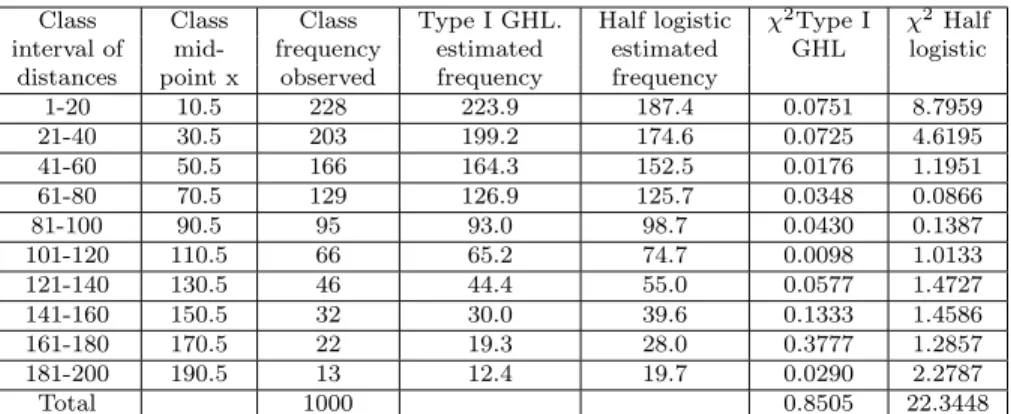
In a cross country race of 200 kilometers, a total of 1000 participants started the race and many stopped on the way without completing the race. The distance covered by each participant before stopping was recorded and a frequency distribution table was constructed to reflect the number of participants that are able to cover an interval of the distance. A probability model that will fit the data is needed. The histogram of the data shows that the data can be analyzed using a type I generalized half logistic or the half logistic distribution of Balakrishnan
and Puthenpura (1986). These two models were fitted to the data and we recommend the one that fits better. The distribution of the data and the analysis are shown in Table 2.
The estimates of the parameters of the type I generalized half logistic distribution as obtained from computer programme are (ˆμ = 0.5, σˆ = 51.4, qˆ = 1.188) while that of the half logistic of Balakrishnan et al are (ˆμ= 0.5,σˆ = 52.74), the outcomes of the analysis are shown in the Table 2.
The adequacy of the model is tested using the method of chi-square test.
From the table below, χ2calculated for the type I generalized half lo-gistic model is 0.8505 while that of half lolo-gistic of Balakrishnan et al is 22.3448. From the table of chi-square, χ2(7,0.05) = 14.0671 and
χ2(8,0.05) = 15.5073. While type I generalized half logistic model is ad-equate for this data, the half logistic model of Balakrishnan et al is inadequate.
Table 2: Analysis of cross country race data
Class Class Class Type I GHL. Half logistic χ2Type I χ2Half interval of mid- frequency estimated estimated GHL logistic
distances point x observed frequency frequency
1-20 10.5 228 223.9 187.4 0.0751 8.7959
21-40 30.5 203 199.2 174.6 0.0725 4.6195
41-60 50.5 166 164.3 152.5 0.0176 1.1951
61-80 70.5 129 126.9 125.7 0.0348 0.0866
81-100 90.5 95 93.0 98.7 0.0430 0.1387
101-120 110.5 66 65.2 74.7 0.0098 1.0133
121-140 130.5 46 44.4 55.0 0.0577 1.4727
141-160 150.5 32 30.0 39.6 0.1333 1.4586
161-180 170.5 22 19.3 28.0 0.3777 1.2857
181-200 190.5 13 12.4 19.7 0.0290 2.2787
Total 1000 0.8505 22.3448
Note: GHL means generalized half logistic.
4
Properties of the type I Generalized Half
Logistic Distribution
4.1 The Median
The median of a probability density function f(x) is a point xm on the real line which satisfies the equation
xm
−∞f(x)dx= 1/2.
This implies that
1−2q(1+ex)−q = 1/2⇒2q(1+ex)−q = 1/2⇒(1+ex)−q = 2−q−1, (4.1) solving forx gives x= ln(2(q+1)/q−1). Therefore the median of a type I generalized half logistic distribution is
xmedian = ln(2(q+1)/q −1) (4.2) which reduces to ln3 whenq = 1, as the median of an ordinary standard half logistic distribution.
4.2 The 100p-Percentage Point
The 100p-percentage point is obtained by setting the cumulative prob-ability distribution function top. That is
F(x(p)) =p⇒2q(1 +ex(p))−q = 1−p. (4.3) Solving for x(p) gives
x(p)= ln[q
2q
1−p−1]. (4.4)
This gives the value of the point x(p) on the real line that produces a percentage p of the distribution.
4.3 The Mode
The mode of a probability density function is obtained by equating the derivative of the density function to zero and solving for the variable. thus,
fX(x;q) =
2qqex
(1 +ex)q+1, 0≤x <∞, q >0.
fX (x;q) = 2qq[(1 +e
x)ex−(q+ 1)e2x
(1 +ex)q+2 ]. (4.5) Equating the derivative to zero, the solution to this equation givesx= −lnq. This gives the mode of the distribution as confirmed when we put
q = 1 which gives the mode of standard half logistic distribution.
5
Characterizations of the Type I Generalized
Half Logistic Distribution
In this section, we present a theorem that relates the type I generalized half logistic distribution to Pareto distribution and also a differential equation whose solution is the probability density function of the type I generalized half logistic distribution is presented.
Theorem 5.1. Let X be a continuously distributed random variable with density function fX(x). Then the random variable Y = ln(2x−1)
is a generalized half logistic random variable if and only if X has a generalized Pareto distribution with parameter q.
Proof. If X is a generalized Pareto distributed random variable with parameters q, then
fX(x;q) = q
xq+1, x >1, q >0. (5.1) Since the random variabley= ln(2x−1) implies thatx= 1+2ey and the Jacobian of the transformation is|J|= 12ey. Therefore
fY(y) = 2
qqey
(1 +ey)q+1, y >0 (5.2) which is the probability density function for type I generalized half lo-gistic distribution.
Conversely, if Y has a type I generalized half logistic distribution with distribution function shown in equation (2.2), then the cumulative distribution function of X is given as
FX(x) =P r[X≤x] =P r[
1 +ey
2 ≤x] =FY[ln(2x−1)] = 1−x
−q.
(5.3) Since equation (5.3) is the distribution function for the generalized Pareto distribution given in equation (5.1), which confirms the result.
Theorem 5.2. The random variable X is type I generalized half logistic with parameter q if and only if the density function f given by equation (2.2) satisfies the homogeneous differential equation
(1 +ex)f+ (qex−1)f = 0, (5.4)
where prime denotes differentiation.
Proof. SupposeXhas a type I generalized half logistic with parameter
q where
fX(x;q) =
2qqex
(1 +ex)q+1,
it is easily shown that the functionf above satisfies equation (5.4). Conversely, we assume thatfsatisfies (5.4). Separating the variables in (5.4) and integrating, we have
f = ke
x
(1 +ex)q+1 (5.5)
where k is a constant. The value of k that makes f a density function is k= 2qq.
Possible Application of Theorem 5.2: From equation (5.4), we have
x= ln( f−f
qf+f)
or equivalently
x= ln( F
−F
qF+F) (5.6)
where F is the corresponding distribution function as shown above. Thus, the importance of Theorem (5.2) lies in the linearizing trans-formation (5.6). The transtrans-formation (5.6) can be regarded as a type I generalized half logistic model alternative to Berkson’s logit transform (Berkson (1944)) and Ojo’s logit transform whenp=q = 1 (Ojo (1997)) for the ordinary logistic model.
Thus in the analysis of bioassay and quanta response data, if model (2.2) is used, what Berkson’s logit transform does for the ordinary lo-gistic can be done for the model (2.2) by the transformation (5.6).
6
Order Statistics from type I Generalized Half
Logistic Distribution
Let X1, X2, ..., Xn be a random sample of size n from the type I
gen-eralized half logistic distribution and let X1:n ≤ X2:n ≤ .... ≤ Xn:n
be the corresponding order statistics. Let FXr:n(x), r = 1,2, ..., n be the cumulative distribution function of therth order statistics Xr:n and
fXr:n(x) denotes its probability density function. David (1970) gives the probability density function of Xr:n as
fXr:n(x) = 1
B(r, n−r+ 1)[F(x)]
r−1[1−F(x)]n−rf(x). (6.1)
For the type I generalized half logistic distribution with parameter
q which has probability density function and cumulative distribution function given in equations (2.2) and (2.3) respectively. By substitution into equation (6.1), we have
fXr:n(x) =
1
B(r, n−r+ 1)[1−2
q(1+ex)−q]r−1[2q(1+ex)−q]n−r 2qqex
(1 +ex)q+1
= 2
q(n−r+1)qex
B(r, n−r+ 1)(1 +ex)qn+1[(1 +e
x)q−2q]n−r. (6.2)
The knowledge of the smallest and largest order statistics are of great importance in statistical studies. They are very useful in the study of extreme values and range.
6.1 The Largest Order Statistics
Consider the probability density of therthorder statistics from the type I generalized half logistic distribution in equation (6.2). Letr =n, then the probability density function of the largest order statistic is
fXn:n(x) = 2
qnqex
(1 +ex)qn+1. (6.3)
Thepthmoment of the largest order statistics from the type I generalized half logistic distribution is
E[Xnp:n] =
xpfXn:n(x)dx= 2qnq
∞
0
xpex
(1 +ex)qn+1dx. (6.4) The above integral is not close but can be evaluated numerically, so with
nknown, we can compute the mean, variance, kurtosis and skewness for a set of largest observations from the type I generalized half logistic distribution.
6.2 The Smallest Order Statistics
Consider the probability density of therthorder statistics from the type I generalized half logistic distribution in equation (6.2). Letr= 1, then the probability density function of the smallest order statistic is obtained as
fX1:n(x) =
2qnqnex
(1 +ex)qn+1[(1 +e
x)q−2q]n−1. (6.5) Using binomial theorem for positive integral exponent,
[(1 +ex)q−2q]n−1 =
n−1
j=0 (−1)j
n−1
j
2q(n−1−j)(1 +ex)qj
and
(1 +ex)qj =
qj k=0 qj k
ex(qj−k).
Therefore
fX1:n(x) = 2
qnqnex
(1 +ex)qn+1
n−1
j=0
(−1)j n−1
j
2q(n−1−j)(1 +ex)qj
= 2qnqnex
n−1
j=0
(−1)j n−1
j
2q(n−1−j)(1 +ex)qj−qn−1
= 2qnqnex
n−1
j=0
(−1)j n−1
j
2q(n−1−j)
qj−qn− 1
k=0
qj−qn−1
k
ex(qj−qn−1−k)
= 2qnqn
n−1
j=0
(−1)j n−1
j
2q(n−1−j)
qj−qn− 1
k=0
qj−qn−1
k
ex(qj−qn−k)
=qn
n−1
j=0
(−1)j n−1
j
2q(2n−1−j)
qj−qn− 1
k=0
qj−qn−1
k
ex(qj−qn−k)
=qn
n−1
j=0
qj−qn− 1
k=0
(−1)j n−1
j
qj−qn−1
k
2q(2n−1−j)ex(qj−qn−k). (6.6)
Thus, thepth moment of X1:n is
E[X1:pn] =θ
∞
0
xpex(qj−qn−k)dx
whereθ=qnnj=0−1kqj=0−qn−1(−1)jn−j1qj−kqn−12q(2n−1−j)
E[X1:pn] =θ
∞
0
xpe−x(qn+k−qj)dx.
Letx(qn+k−qj) =t,x=t/(qn+k−qj) anddx=dt/(qn+k−qj), then
E[X1:pn] =θ
∞
0
( t
qn+k−qj)
pe−t dt
qn+k−qj
= θ
(qn+k−qj)p+1
∞
0
tpe−tdt= θΓ(p+ 1) (qn+k−qj)p+1 =
p!θ
(qn+k−qj)p+1. (6.7) Hence, to obtain the first, second, third and fourth moments of the smallest order statistics from the type I generalized logistic distribution, we use the equation (6.7) for p = 1,2,3, and 4. The values of these moments can be used to calculate the mean, variance, skewness and kurtosis of the smallest order statistics from the type I generalized half logistic distribution.
6.3 rth Order Statistics from the Type I Generalized Half
Logistic Distribution
Consider the probability density function of therthorder statistics from type I generalized half logistic distribution derived earlier in equation (6.2) as
fXr:n(x) =
2q(n−r+1)qex
B(r, n−r+ 1)(1 +ex)qn+1[(1 +e
x)q−2q]n−r.
By binomial theorem,
[(1 +ex)q−2q]n−r=
n−1
j=0 (−1)j
n−r
j
2q(n−r−j)(1 +ex)qj. (6.8)
Therefore
fXr:n(x) = 2
q(n−r+1)qex
B(r, n−r+ 1)(1 +ex)qn+1
n−1
j=0
(−1)j n−r
j
2q(n−r−j)(1 +ex)qj
= 2
q(n−r+1)qex
B(r, n−r+ 1)
n−1
j=0
(−1)j n−r
j
2q(n−r−j)(1 +ex)qj−qn−1. (6.9)
Also by expanding (1 +ex)qj−qn−1 binomially,
(1 +ex)qj−qn−1=
qj−qn−1
k=0
qj−qn−1
k
ex(qj−qn−1−k). (6.10)
Substituting back intofXr:n(x), we have
fXr:n(x) =
2q(n−r+1)qex B(r, n−r+ 1)
n−1
j=0 (−1)j
n−r
j
2q(n−r−j)
×
qj−qn−1
k=0
qj−qn−1
k
ex(qj−qn−1−k)
= q
B(r, n−r+ 1)
n−1
j=0
qj−qn−1
k=0
(−1)j
n−r
j
×
qj−qn−1
k
2q(2n−2r−j+1)ex(qj−qn−k). (6.11)
The pth moment of X(r:n) from the type I generalized half logistic distribution is then obtained as
E[Xrp:n] = Λ
∞
0
xpex(qj−qn−k)dx= Λ
∞
0
xpe−x(qn+k−qj)dx (6.12)
where
Λ = q
B(r, n−r+ 1)
n−1
j=0
qj−qn−1
k=0
(−1)j
n−r
j
qj−qn−1
k
2q(2n−2r−j+1).
Therefore,
E[Xrp:n] = ΛΓ(p+ 1)
(qn+k−qj)p+1. (6.13) The expression for this moment can be used to calculate the mean, variance, skewness and kurtosis of therth order statistics from the type I generalized half logistic distribution.
References
Balakrishnan, N. (1985), Order statistics from the Half Logistic Distri-bution. Journal of Statistics and Computer Simulation, 20, 287-309.
Balakrishnan, N. and Puthenpura, S. (1986), Best Linear Unbiased Estimators of Location and Scale Parameters of the Half Logistic Distribution. Journal of Statistical Computation and Simulation, 25, 193-204.
Balakrishnan, N. and Leung, M. Y. (1988), Order statistics from the Type I generalized Logistic Distribution. Communications in Statis-tics - Simulation and Computation, 17(1), (1988), 25-50.
Balakrishnan, N. and Wong, K. H. T. (1991), Approximate MLEs for the Location and Scale Parameters of the Half-Logistic Distribu-tion with Type-II Right-Censoring. IEEE TransacDistribu-tions on Relia-bility, 40(2), 140-145.
Berkson, j. (1994), Application of the logistic function to bioassay. Journal of the American Statistical Association, 39, 357-365. David, H. A. (1970), Order Statistics. New York: John Wiley.
Ojo, M. O. (1997), Some Relationships between the generalized logistic and other distributions. Statistica, LVII(4), 573-579.
Olapade, A. K. (2003), On Characterizations of the Half Logistic Distri-bution. InterStat, February Issue,2, http://interstat.stat.vt.edu/ InterStat/ARTICLES/2003articles/F06002.pdf
Torabi, H. and Bagheri, F. L. (2010), Estimation of Parameters for an Extended Generalized Half Logistic Distribution Based on Com-plete and Censored Data. JIRSS,9(2), 171-195.