AENSI Journals
Australian Journal of Basic and Applied Sciences
ISSN:1991-8178Journal home page: www.ajbasweb.com
Corresponding Author: M.N. Annuar, Mechanical Engineering Department, Universiti Teknologi PETRONAS, 31750 Tronoh, Perak,, Malaysia
A Comparative Analysis of Optical Flow Algorithms for Velocimetry
M.N. Annuar and M. Ovinis
Mechanical Engineering Department, Universiti Teknologi PETRONAS, 31750 Tronoh, Perak,, Malaysia
A R T I C L E I N F O A B S T R A C T Article history:
Received 30 September 2014 Received in revised form 17 November 2014 Accepted 25 November 2014 Available online 13 December 2014
Keywords:
Optical flow, flow rate estimation, computer vision.
The use of an optical method for velocimetry is important where it is not possible to use invasive flow measurement techniques,as is the case in a hydrocarbon leak from a ruptured subsea pipeline. However, measurements of the velocity of fluids optically is inherently difficult due to dense fluid motion and lack of distinct features. Timothy J. Crone (Crone et al, 2008) developed a system based on optical plume velocimetry, an optical flow technique, to determine flow rates using image analysis. In this paper, the performance of three optical flow algorithms, iterative Lucas-Kanade, Horn-Schunk and Brox based onwarping theory, for optical plume velocimetry were assessed. Crone’s experimental setup was replicatedand the accuracy of the three algorithms at three different flow rates were assessed. The Brox optical flow algorithm, based on theory of warping, was the most accurate, with an average error of 8.6%.
© 2014 AENSI Publisher All rights reserved. To Cite This Article: M.N. Annuar and M. Ovinis., A Comparative Analysis of Optical Flow Algorithms for Velocimetry. Aust. J. Basic & Appl. Sci., 8(24): 170-174, 2014
INTRODUCTION
As the oil and gas industry venturesfurther deep water to keep up with the world’s energy demand,leaks from ruptured pipelines are inevitable, despite tight safety measures. An accurate estimate of the leak flow rate is necessary asinterventions are based on the flow rate.A recent example is the Deepwater Horizon oil spill on April 20, 2010 in the Gulf of Mexico at an approximate water depth of 1500 metres(Command, 2011). The tragedy which caused the death of 11 workers and millions of barrel of spilled oil. It is regarded as the largest accidental marine oil spill in the history of the industry.There wasa dispute between the well operator, BP and the United States Government on the amount of spilt oil, since there were no proven methods in accurately predicting its volume. Various ad hoc methods were employed to predict the flow rate of hydrocarbon escaping from the leakage,with the most accurate method that by Crone et al(Crone, McDuff, & Wilcock, 2008) using an optical flow based on optical plume velocimetry.
Methodology:
Fig. 1: Experiment Setup(Crone, McDuff, & Wilcock, 2008).
A total of 9 videos wereanalysed, 3 videos each for 100%, 50%, and 25% nozzle opening. The camera specifications used for video recording was as shown in Table 1.
Table 1: Camera Properties.
Camera Model Nikon Coolpix L820
Effective Pixels 16 Million
Sensor Size 1/2.3”
Video Recording Full HD: 1920x1080p
Frame Rate 30fps
ISO Sensitivity ISO125-1500;ISO3200(Auto Mode)
Video Analysis:
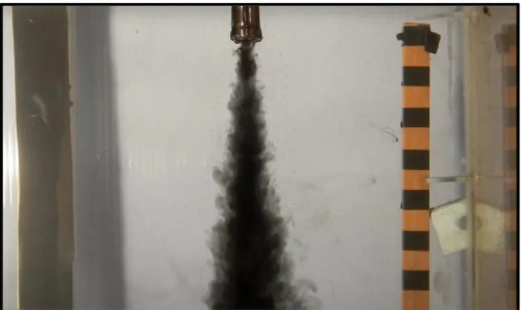
The raw data produced from the video were RGB images.A sample image for a 100% valve opening is shown in Figure 2.
Fig. 2: An RGB image ofthe flow at 100% valve opening extracted from a video recording.
(a) (b)
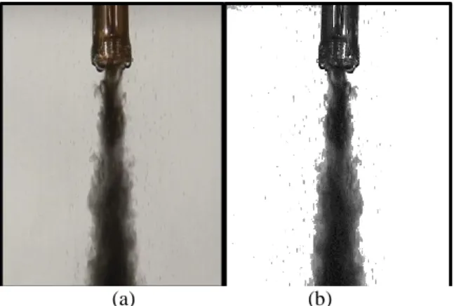
Fig. 3: Cropped sample RGB image (a) and the corresponding Kittler-Illingworth thresholded image (b).
Several thresholding algorithm that were considered such as Bradley’s Adaptive Thresholding (Bradley, 2006), Gray Image Thresholding using Triangle Method, and Illingworth (Kittler, 1986). Kittler-Illingworth thresholding algorithm was chosen as it manages to preserve the profile of the fluid flow while eliminating noise in the image. The thresholding of Kittler-Illingworth’s come from a mixture of two normal distributions having mean and variances, and their respective proportions. It models the two resulting pixel populations, foreground and background, one from those pixels whose brightness level is smaller than threshold and the other with the higher value than the threshold. The value of threshold chosen is based on a value which minimizes the criterion function of the image, automatically givinga recommended threshold level of a given image. The threshold level for the sample imageusing this method was a grayscale level of 171 and the resultant image is shown in Figure 3. As can be seen, the thresholded image retains most of the profile of the flow while eliminating the background noise.
Optical Flow:
The flow rate (pixel/frame) was determined based on several optical flow algorithms applied to the thresholdedimages. The algorithms included in this study are Iterative Lucas-Kanade, Horn-Schunk and Brox based on Warping Theory. The resulting flow rate will be compared to the actual flow rate obtained from volume of fluid displaced over time. Table 2 shows the experimental results. The example shown for the conversionof flow rate to velocimetry (p/f) was for 100% valve opening. The summary of all actual flow rate was shown in Table 3.
Table 2: Experimental Flow Rates.
No Valve Opening (%) Displaced height, h (cm) Area, A (cm2) Time Taken, t(s)
1 100 0.5 5625 120
2 50 0.4 5625 120
3 25 0.3 5625 120
𝑉𝐷 = 𝐴 𝑥 ℎ (1)
where,VD= Displaced Volume (cm3), A = Area of Container (cm2), h = Displaced height (cm)
∴ 𝑉𝐷 = 5625𝑐𝑚2 × 0.5𝑐𝑚 = 2812.5cm3
𝑉 =𝑉𝐷
𝑡 (2)
where,𝑉 = Volumetric flow rate (cm3/s), VD= Displaced Volume (cm3), t = time taken (s)
∴ 𝑉 =2812.5𝑐𝑚
3
120𝑠 = 23.43 𝑐𝑚
3
𝑠
As the radius of nozzle is 0.8cm, the marker besides the nozzle serve as an indicator to determine the relationship between pixels and the length. It was determined that 72 pixels are equivalent to one centimetre. The camera used in the experiment had the speed of 30 frame/s as shown in Table 1. Thus, the velocimetry (p/f) can be calculated by using the given information.
r = 0.8cm 1cm=72pixels
𝑣𝑓/𝑠= 30frame/s
𝑣 = 𝑉
𝐴𝑛𝑜𝑧𝑧𝑙𝑒 (3)
where,𝑣= fluid velocity (cm/s), 𝑉 = Volumetric flow rate (cm3/s), Anozzle = Cross-sectional area of nozzle (cm 2
∴ 𝑣 =23.43 𝑐𝑚
3
𝑠
𝜋(0.82) = 11.65 𝑐𝑚 𝑠
𝑣𝑝/𝑓=
𝑣
𝛼 𝑣𝑓/𝑠 (4)
where,𝑣𝑝/𝑓= velocimetry (pixel/frame), 𝑣= fluid velocity (cm/s), 𝛼= centimetre per pixel constant (cm/pixel),
𝑣𝑓/𝑠= speed of camera (frame/s)
∴ 𝑣𝑝/𝑓= 11.05 𝑐𝑚 𝑠
( 1𝑐𝑚
72𝑝𝑖𝑥𝑒𝑙𝑠)(30
𝑓𝑟𝑎𝑚𝑒 𝑠
)= 27.9
𝑝 𝑓
Table 3: Flow rate.
No. Nozzle Opening (%) Volumetric Flow Rate, , 𝑉 (cm3/s) Fluid Velocity, 𝑣 (cm/s) Velocimetry, 𝑣𝑝/𝑓 (p/f)
1. 100 12.5 11.7 26.5
2. 50 10.5 9.3 22.4
3. 25 7.9 7.0 16.7
Iterative Lucas-Kanade Optical Flow Algorithm:
The iterative Lucas-Kanade(Bouguet, 2001) is a feature tracking based algorithm which has the two key elements of accuracy and robustness. The accuracy component is related to the accuracy of local sub-pixel assigned to be tracked. In order to avoid smoothing the details of the images, a small integration window is need to preserved details in the images. However, the robustness component need a large integration window for better tracking sensitivity with respect to lighting and the image size. Hence, iteration is needed to balance the size of integration window for an optimum result. The feature selection in the algorithm is generalized in 5 steps(Bouguet, 2001) which are:
1. Compute the size of the image and its minimum eigenvalue at every pixel of the image. 2. Set the maximum eigenvalue in the image as the general eigenvalue for the whole image. 3. Retain the image pixel (tracked object) that is within the eigenvalue.
4. Retain the local maximum pixel of the retained feature.
5. Retain the subset of the pixel so that the minimum distance between pair of pixels is larger than threshold distance.
Horn-Schunck Optical Flow Algorithm:
Horn-Schunk(Corpetti, Heitz, Arroyo, & Memin, 2005) is a variational-based algorithm, capable of extracting the dense motion field of a fluid flow. The computation of its velocimetry is based on spatiotemporal derivatives of image intensity, with assumption of continuous image domain in space and time. The algorithm takes the whole image into account in estimating the vectorial continuous function representing velocity field. The technique is able to overcome the limitation of a feature-based algorithm, such as loss of the features due to the incorrect interrogation window, bias towards the lower displacements and higher seeded sub-regions as a result of more frequent pairing, with only the most probable displacement extracted for interrogation.
Warping Theory:
Warping theory by Brox(Brox, Bruhn, Papenberg, & Weickert, 2004) is a variational-based algorithm with improvement over the Horn-Shunk algorithm. Warping theory uses variational-based algorithm smoothness assumption to provide spatiotemporal continuity in the image domain. The algorithm implements non-linearized optical flow constraint integration usinga warping technique. Complementing the grey value constancy assumption is the gradient constancy assumption in order to make the algorithm robust to the changes in grey values. Gradient constancy assumption is important when there are changes in the grey values due to the aperture changes.
Results:
and Warping Theory is a variational-based algorithm which uses smoothness for the resulting flow field to provide continuity in the image domain. The approaches compute the optical flow field for all pixels within the image, and the resultant is a dense optical flow field.
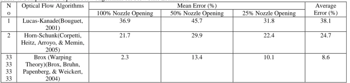
Table 4: Comparison of Optical Flow Algorithms for Flow Rate Estimation. N
o
Optical Flow Algorithms Mean Error (%) Average
Error (%) 100% Nozzle Opening 50% Nozzle Opening 25% Nozzle Opening
1 Lucas-Kanade(Bouguet, 2001)
36.9 45.7 31.8 38.1
2 Horn-Schunk(Corpetti, Heitz, Arroyo, & Memin,
2005)
21.7 29.9 22.4 24.7
33 33 33 33
Brox (Warping Theory)(Brox, Bruhn, Papenberg, & Weickert,
2004)
2.3 13.4 10.1 8.6
Brox, which is based on warping theory, is a variation al-based algorithm as it incorporates a gradient constancy assumption for the robustness of the algorithm. As shown in Table 4,it has the best accuracy of all three algorithms considered. However further study should be done to investigate the effect of smoothness constant in variation al-based algorithms.To measure the flow rate of hydrocarbon leakage, the actual deep water conditions e.g. high pressures and low temperatures, need to be replicated. In addition, video recordings will be susceptible to sway due to sea current; resulting in slight changes in the angle of view, which will affect the overall accuracy. Thus, the effect of sway should be considered for robustness. Additionally, the usage of high speed camera would be beneficial to the development of the system, as the flow rate could be in estimated more accurately, albeit at the expense of computation cost as there will be vast amount of information to be processed.
Conclusion:
A comparative analysis of three optical flow algorithms for optical plume velocimetrywas performed at three different flow rates to investigate the accuracy of each algorithm. The three optical flow algorithms investigated were Iterative Lucas-Kanade, Horn-Schunk, and Brox based on warping theory. Of the three algorithms considered, the Brox optical flow algorithm, based on theory of warping, was the most accurate, with an average error of 8.6%.
REFERENCES
Bouguet, J., 2000. Pyramidal implementation of the lucas kanade feature tracker. Intel Corporation, Microprocessor Research Labs.
Brox, T., A. Bruhn, N. Papenberg, J. Weickert, 2004. High accuracy optical flow estimation based on a theory for warping. In Computer Vision-ECCV 2004 (pp. 25-36). Springer Berlin Heidelberg.
Command, D.H., 2011. US scientific teams refine estimates of oil flow from BP’s well prior to capping. Gulf of Mexico Oil Spill Response 2010.
Corpetti, T., D. Heitz, G. Arroyo, E. Memin, A. Santa-Cruz, 2006. Fluid experimental flow estimation based on an optical-flow scheme. Experiments in fluids, 40(1): 80-97.
Crone, T.J., R.E. McDuff, W.S. Wilcock, 2008. Optical plume velocimetry: A new flow measurement technique for use in seafloor hydrothermal systems. Experiments in Fluids, 45(5): 899-915.