Short-term wind power prediction based on extreme learning machine with error correction

O R I G I N A L R E S E A R C H

Open Access

Short-term wind power prediction based

on extreme learning machine with error

correction

Zhi Li

, Lin Ye

, Yongning Zhao

, Xuri Song

, Jingzhu Teng

and Jingxin Jin

Abstract

Introduction:Large-scale integration of wind generation brings great challenges to the secure operation of the power systems due to the intermittence nature of wind. The fluctuation of the wind generation has a great impact on the unit commitment. Thus accurate wind power forecasting plays a key role in dealing with the challenges of power system operation under uncertainties in an economical and technical way.

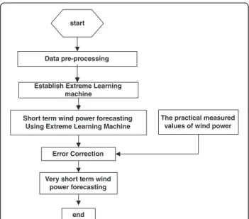
Methods:In this paper, a combined approach based on Extreme Learning Machine (ELM) and an error correction model is proposed to predict wind power in the short-term time scale. Firstly an ELM is utilized to forecast the short-term wind power. Then the ultra-short-term wind power forecasting is acquired based on processing the short-term forecasting error by persistence method.

Results:For short-term forecasting, the Extreme Learning Machine (ELM) doesn’t perform well. The overall NRMSE (Normalized Root Mean Square Error) of forecasting results for 66 days is 21.09 %. For the ultra-short term

forecasting after error correction, most of forecasting errors lie in the interval of [−10 MW, 10 MW]. The error distribution is concentrated and almost unbiased. The overall NRMSE is 5.76 %.

Conclusion:The ultra-short-term wind power forecasting accuracy is further improved by using error correction in terms of normalized root mean squared error (NRMSE).

Keywords:Ultra-short-term forecasting, Wind power forecasting, Extreme Learning Machine, Error correction

Introduction

Wind power has been undergoing a rapid development in recent years. The large-scale integration of wind power is challenging power grids operation and management [1]. Compared with conventional generation, one of the lar-gest problems of wind power is its dependence on the volatility of the wind [2]. Unexpected variations of wind generation may increase operating costs, increasing re-serves requirements, and posing potential risks to system reliability. In order to schedule the spinning reserve cap-acity and manage the grid operation, persistence approach was commonly used to predict changes of the wind power production in the ultra-short-term [3, 4].

Wind power is impacted by wind speed, temperature, hu-midity, latitude, terrain topography, air pressure, and other factors [5]. Modeling the behavior of wind is a challenge due to its stochastic nature. The existing forecasting methods can be mainly classified as physical approaches, statistical approaches, as well as a combination of both [6]. The physical models use physical considerations, such as meteorological (numerical weather predictions), and topo-logical (orography, roughness, obstacles) information and technical characteristics of the wind turbines (hub height, power curve, thrust coefficient) [7]. Statistical models find the relationships between a set of explanatory variables in-cluding NWP results and online measured generation data [7]. The basic statistical approach includes the time-series analysis and neural networks, such as Box-Jenkins ARMA (p,q) models, whereprepresents most recent wind speeds andqrepresents most recent forecasting errors [8]. Neural network (NN) models have been widely applied in a variety * Correspondence:[email protected]

1_{College of Information and Electrical Engineering, China Agricultural}

University, P. O. Box 210, Beijing 100083, Peoples Republic of China Full list of author information is available at the end of the article

of business fields including accounting, management infor-mation systems, marketing, and production management. Many researchers focus on the improvement of NN, in-cluding recurrent NN, deep NN and so on [9–14]. Extreme Learning Machine(ELM) is based on a single-hidden layer feed-forward neutral network and only needs to calculate random weight between inputting layer and hidden layer. The performance of ELM is better than traditional NN in terms of numerical experiments. Furthermore, the com-bined models have been widely used to improve wind power forecasting accuracy. Wind power forecasting method based on empirical mode decomposition (EMD) and support vector machine (SVM) was proposed to cope with the nonlinearity and non-stationarity of wind speed data. The combined approach can improve the forecasting accuracy by 5–10 % compared to single statistics [15].

Several wind power forecasting tools have been devel-oped across the world. A Wind Power Prediction Tool (WPPT) is developed to predict the wind power on various time scales, from half an hour to 36 h ahead. This tool is based on adaptive recursive least square estimation with ex-ponential forgetting factor [16]. The WPPT can forecast the wind power production in relatively large geographical re-gions. For each individual wind farm, it uses statistical models to describe the relationship between observed power production and the weather predictions. Another tool named as the Prediktor developed at Risø mainly uses physical relations to transform the predicted wind into pre-dicted power [17]. The Zephyr tool is the combination of the Wind Power Prediction Tool (WPPT) and Prediktor tool and its main goal is to merge Prediktor and WPPT to obtain synergy between the physical and the statistical ap-proach [17]. The Sipreolico tool, developed by the Univer-sity of Carlos III of Madrid, consists of nine adaptive nonparametric statistical models that are recursively esti-mated with either the recursive least squares algorithm or a Kalman filter. The tool is based on Spanish HIRLAM fore-casts, taking into account hourly SCADA data from 80 % of all Spanish wind turbines [18]. The EWIND model de-veloped by TrueWind, Inc. applies a once-and-for-all parameterization for the local effect by using the output of the ForeWind NWP model, and it uses either a multiple screening linear regression model or a Bayesian neural net-work to find out the systematic errors [19]. The Advanced Wind Power Prediction tool (AWPT) was developed by ISET (the institute of “Solare Energieversorgungstechnik”) and the tool uses weather forecasts coming from Lokalmo-dell (LM) of the Deutsche Wetterdienst (DWD) and pre-dicts the wind power with artificial neural networks [20]. Ecole de Mines de Paris (ARMINES) and Rutherford Ap-pleton Laboratory (RAL) have developed models for short-term prediction based on fuzzy-neural networks [20].

The individual forecasting method cannot achieve a high accuracy due to the intrinsic characteristics of wind

speed and wind power. In this paper, a combined statis-tical approach for wind power forecasting is presented by using Extreme learning method and error correction. The ultra-short-term power forecasting is acquired based on processing the forecasting error of short-term forecasting results based on the persistence method in terms of Normalized Root Mean Square Error (RMSE).

Methods

Extreme Learning Machine (ELM)

ELM theory was proposed to predict wind power, which tends to provide good generation and performance at ex-tremely fast learning speed in theory and practical applica-tions. ELM has the following several advantages:

1) The parameters of ELM can be set easily, and ELM originally can get a good performance only with fitful references in hidden layers.

2) The computation of ELM is efficient, which does not need as many iterations as Neural Network (NN) and as complexity as Support Vector Machine (SVM) in when solving quadratic optimization. 3) ELM has good generalization performance. And the

experimental results show that the ELM can achieve good generalization performance in most cases and can learn faster than feed-forward neural networks [21].

Now the EML has been widely used in several fields such as face recognition, image classification,wind pre-diction in short-term scale. Wind power forecasting can be regarded as an ELM problem, because some factors such as wind speed, air condition, temperature & hu-midity, wind turbine arrangement have influence on wind production. As for how they exactly affect wind production has not been clearly known [22]. ELM model can be established by using example data and predict the curve of power in short-term.

The ELM model is based on a single-hidden layer feed-forward neural network (SLFN). The advantage of the ELM algorithm is that it distributes the weights and thresholds between the inputting layer and the hidden layer in random and does not need to adjust these ran-dom parameters during the whole learning process so that it can complete the training process extremely fast. Based the above advantage, ELM is chosen as a predictor to predict day-ahead wind power in the short-term time scale. The structure of a standard ELM network is demonstrated in Fig. 1.

The main parameters of ELM are described as follow:

ω¼

ω11 ω12 ⋯ ω1n

ω21 ω22 ⋯ ω2n

⋮ ⋮ ⋮ ⋮

ωl1 ωl2 ⋯ ωln

2 6 6 4

3 7 7 5

ln

where ‘ω’is the network weight between the input layer and the hidden layer, and‘ωij’is the weight between theith

input node of the input layer and thejthhidden node of

the hidden layer.‘l’is the number of input nodes in input layer.‘n’is the number of hidden nodes in output layer.

β¼

β11 β12 ⋯ β1m β21 β22 ⋯ β2m

⋮ ⋮ ⋮ ⋮

βl1 βl2 ⋯ βlm 2 6 6 4 3 7 7 5

lm

ð2Þ

where the‘β’is the network weight between the hidden

layer and the output layer, and‘βij’is the weight between the ithhidden node of the hidden layer and the jth

hid-den node of the output layer. ‘m’is the number of

out-put nodes in outout-put layer.

b¼½b1 b2 ⋯ bl−l11 ð3Þ

where‘b’is the threshold of the hidden layer.

X is supposed to be the input matrix and the history dataXare used to train the ELM network.

X¼

x11 x12 ⋯ x1p

x21 x22 ⋯ x2p

⋮ ⋮ ⋮

xn1 xn2 ⋯ xnp

2 6 6 4 3 7 7 5

np

ð4Þ

The real outputting matrix of the ELM network can be defined as below:

T¼½t1 t2 ⋯ tp_mp ð5Þ

And based on the equations (1)–(4), the real output-ting matrix of the ELM can be defined as follow:

tj¼ t1j

t2j

⋮ tmj 2 6 6 4 3 7 7 5

m1

¼ Xl

i¼1

βi1g ωiXjþbi

Xl

i¼1

βi2g ωiXjþbi

⋮

Xl

i¼1

βimgωiXjþbi 2 6 6 6 6 6 6 6 6 6 6 4 3 7 7 7 7 7 7 7 7 7 7 5

m1

;ðj¼1;2;3; ::::::;pÞ

ð6Þ

where

ωi ¼½ωi1 ωi2 ⋯ ωin ð7Þ

Xj¼x1j x2j ⋯ xnjT ð8Þ g(x) is an activation function in the hidden layer of the ELM.

The following equations can be acquired by Eqs. (5)–(8):

^

β¼H−1_TT _ð9Þ

where

Hω1;ω2;⋯;ωl;b1;b2;⋯;bl;X1;X2;⋯Xp

¼

gðω1⋅X1þb1Þ gðω2⋅X1þb2Þ ⋯ gðωl⋅X1þblÞ gðω1⋅X2þb1Þ gðω2⋅X2þb2Þ ⋯ gðωl⋅X2þblÞ

⋮ ⋮ ⋮ ⋮

gω1⋅Xpþb1 g ω2⋅Xpþb2

⋯ gωl⋅Xpþbl

2 6 6 4 3 7 7 5

ð10Þ

AndH−1is pseudo-inverse matrix ofH. The ELM can be solved in the following algorithm:

Algorithm ELM: Given a training set {(X,T)|X∈Rn×p, T∈Rm×p_{}, activation functiong(x), testing setX^ and} hid-den node numberp.

Step one: Randomly assign input weightωand biasb. Step two: Calculate the hidden layer output matrixH. Step three: Calculate the output weight matrixβ. Step four: Input matrix X^ and get the output testing results by the transform (9).

Error correction

Based on the ELM forecasting results, an error cor-rection model is applied to obtain the ultra-short-term forecasting. The persistence method is used as a benchmark model to examine whether an advanced model can perform well. In this model the future

wind power will be the same as occurred in the present time step as given by

^

Ptþkjt¼Pt ð11Þ

where P^tþkjt is the forecast at time tfor the look-ahead timekandPtis the measurement at timet.

In comparison with wind power, the temporal char-acteristics of wind power forecasting errors are less mentioned in literatures. However, it is found that the forecasting error level at next time point tends to keep the same as present time point by analyzing the states transition probability among different error levels. Thus, the error for next time point can be written as

^etþ1jt ¼et ð12Þ

where et is the deviation between forecasted and

mea-sured wind power.

et¼pt−^ptjt−1 ð13Þ

The computed error is then added to the forecasted wind power for next time point to get the corrected forecasting.

~

p_tþ1jt¼^p_tþ1jtþ^etþ1jt¼^ptþ1jtþet ð14Þ

The flow chart of wind power forecasting procedure is shown in Fig. 2.

Data description and pre-processing

The proposed model is verified using the measured data in a wind farm located in the northern China for a period of about 15 months from 24 February 2014 to 31 May 2015. The 41072 non-consecutive data points before 02 March 2015 are used for train-ing the ELM models whereas the consecutive time series of 66 days from 02 March 2015 to 31 May 2015 is used to verify the models performances. The total installed capacity of the wind farm is 50 MW. The measured data are used for both training the ELM model and verifying the model. The time scale of collecting data is 15 min. The scatter of wind power versus wind speed of the wind farm is plotted in Fig. 3.

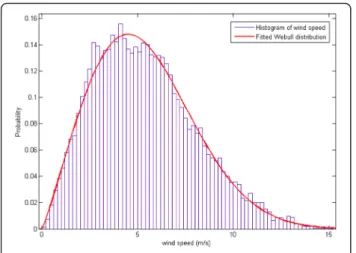
The characteristic of wind speed is shown as the fre-quency histogram in Fig. 4. It can be well fitted using a Webull distribution.

The mechanical power extracted from wind by a wind turbine is a function of the wind speed, blade pitch angle, and shaft speed. The algebraic equation shown below characterizes the power extracted [23].

Pm¼1 2ρv

3

wπr2Cpð Þλ ð15Þ

wherePmis the power extracted from the wind, in watts;

ρ the air density, in kg/m3; r the radius swept by the

rotor blades, in m; vw the wind speed, in m/s; Cp the

performance coefficient; λ the tip ratio, i.e., the ratio of turbine blade speed to that of the wind

λ¼ω_vtr

w ð16Þ

whereωis mechanical rotor speed in radians/s.

From Eq. (15) it is noted that the air density, the wind speed are not quantities that can be con-trolled. That means a wind turbine will yield

Fig. 3Scatter plot of wind power versus wind speed

different wind power output even at the same wind speed. A wind farm comprises tens or even hun-dreds of turbines, which making the relationship be-tween the farm output and speed much weaker than that of a wind turbine. Even so, the wind power output depends on wind speed obviously, as shown in Fig. 3. The object of modeling an ELM is to characterize such kind of implicit dependence. However some anomalous data exists in the original datasets, which will have negative influence on the wind power forecasting accuracy. Two kinds of anomalies are supposed to be eliminated before building an ELM model.

1) When the wind speed is very large (e.g. larger than 5 m/s) but the corresponding wind power is close to zero.

2) When the wind speed is close to zero but the wind farm output is very large (e.g. larger than half of the rated capacity of the wind farm).

Moreover, wind speed and power data are normalized by using the following formula

xnormal¼ x−maxð Þx

maxð Þx −minð Þx ð17Þ

where x is the original data, xnormal is the normalized

data, max(x) is the maximum of original datasets, and

min(x) is the minimum of original datasets.

Fig. 7Ultra-short-term forecasting results and their corresponding measurements after error correction

Fig. 6Short-term forecasting results of ELM and their corresponding measurements

Fig. 5NRMSE for day-ahead forecasting by ELM models with different hidden nodes number

Results and discussion Model parameterization

The input of the ELM model is wind speed and the out-put is wind power, hence the number of nodes for both of input layer and output layer is set as one. As for the hidden layer, different values of the hidden nodes num-ber are tested. The criterion for quantifying the perform-ance of wind power forecasting is normalized root mean squared error (NRMSE).

NRMSE¼

ffiffiffiffiffiffiffiffiffiffiffiffiffiffiffiffiffiffiffiffiffiffiffiffi Xn

i¼1

p_i−^p_i

ð Þ2

s

Cap⋅pffiffiffin ð18Þ

NRMSE for day-ahead (24 h-ahead) forecasting by ELM models with different hidden nodes number are shown in Fig. 5.

From Fig. 5 it can be seen that, the value of NRMSE decreases dramatically when the hidden nodes number ranges from 1 to 3. With 3 hidden nodes, the ELM has the best performance of 21.09 % in terms of NRMSE. Adding more nodes will not lead to better results. Thus, the nodes number is finally set to be 3.

Results and analysis

The day-ahead forecasting results in short-term scale be-fore error correction by using ELM and their corre-sponding measurements dated from 22 April 2015 to 23 April 2015 are shown in Fig. 6. The 15 min-ahead fore-casting results in ultra-short-term scale and their corre-sponding measurements after error correction are shown in Fig. 7.

In Fig. 6, the ELM doesn’t perform well due to the strong stochastic feature of wind and the weak relation-ship between wind farm output and wind speed. Particu-larly, the ramp events are not accurately forecasted. It can be seen that large errors occur around peak value of measurement curve, where wind power changes drastic-ally in a short time. The overall NRMSE of forecasting results for 66 days is 21.09 %.

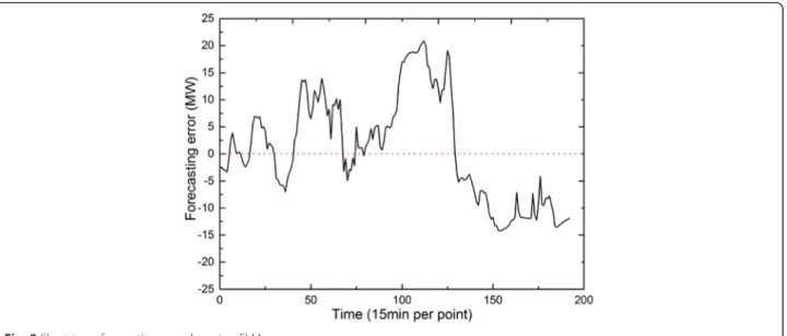
The short-term forecasting errors are shown in Fig. 8 and their distribution is shown in Fig. 9. Ultra-short-term forecasting error after error correction is depicted in Fig. 10. As can be seen from Fig. 10, the forecasting error fluctuates drastically with large amp-litude. The maximal error reaches up to 50 % of in-stalled capacity of the wind farm. It is noted that from Fig. 8, though most of the errors lie in the interval of [−20 MW, 20 MW], there is still a portion of large errors that cannot be neglected. It is indi-cated that the spread range of errors distribution is

Fig. 9Short-term forecasting error distribution by using ELM

large and positively biased, which reveals the poor forecasting performance.

While in Fig. 7 the ultra-short-term forecasting curve follows closely with the measurement curve. In addition, Figs. 10 and 11 show that most of fore-casting errors lie in the interval of [−10 MW, 10 MW]. The distribution is concentrated and almost unbiased. The overall NRMSE is 5.76 %, indicating a good result of the correction method for ultra-short-term forecasting.

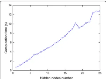
In terms of the computational efficiency, time con-sumed for training and testing ELM models with varying hidden nodes number is depicted in Fig. 12.

It is noted that the computation time is approxi-mately proportional to the hidden nodes number. When the hidden nodes number is 3, the computa-tion time is 1.5377 s, including the time for training model with 41072 data points and forecasting 6336 data points. That indicates a high computational

efficiency for wind power forecasting, which can sat-isfy the practical needs.

Conclusions

In this paper, an extreme learning machine model with error correction with higher efficiency is developed to predict power output of a wind farm in a term time scale. Case study shows that the ultra-short-term wind forecasting accuracy is further improved in terms of normalized root mean squared error (NRMSE).

About the Authors

Zhi Liwas born in Hubei, China, in 1994. She received her B.Sc. in applied mathematics from Department of Math, China Agricultural University in 2015. She is currently a PhD student of the Department of Electric Power Systems, China Agricultural University(CAU), Peoples Republic of China. Her research interests are wind power forecasting, model predictive control(MPC) in wind power operations.

Lin Ye(M_’98) received his B.Sc. from WuHan University of Hydraulic & Electric Engineering, Peoples Republic of China in 1992 and his Ph.D. degree in 2000 from the Institute of Electrical Engineering (IEE), Chinese Academy of Sciences (CAS), all in electrical engineering. He has been pursuing research at ForschungsZentrum Karlsruhe(FZK) (*now merged with University of Karlsruhe(TH) to form Karlsruhe Institute for Technology,KIT) as a research fellow of Alexander von Humboldt Stiftung/Foundation (AvH) of Germany from 2000 to 2002. In 2004, Dr. Lin Ye joined the Interdisciplinary Research Center (IRC) in Superconductivity, Department of Engineering/Cavendish Laboratory, The University of Cambridge, United Kingdom, as a research fellow. At Cambridge Laboratory, he had been involved in developing a novel resistive type of superconducting fault current limiter prototype for electrical marine propulsion which was funded by Rolls-Royce Plc and the Department of Trade & Industry (DTI) of the United Kingdom. He received the“Hua Wei”Award from Chinese Academy of Sciences in 1999, and Research Young Investigator Award from Fok Ying Tung Education Foundation, Ministry of Education, Peoples Republic of China in 2003. He was an awardee of the Program for New Century Excellent Talents in China Universities in 2008. He is currently a full professor in electrical power engineering at the Department of Electric Power Systems, China Agricultural University (CAU), Beijing, Peoples Republic of China, where he has headed the Power System Off-line/Real Time Simulations Laboratory. Dr. Lin Ye holds memberships in IEEE (USA), and European EMTP-ATP Users Group (EEUG) as well as senior member of Wolfson College at Cambridge University. He is also a member of the IEEE Task Force on Sustainable Energy Systems for Developing Communities. His research interests are in the areas of electrical power

Fig. 12Computation time for training and testing ELM models with varying hidden nodes number

Fig. 11Ultra-short-term forecasting error distribution after error correction

system analysis & control, Electromagnetic Transient Program (EMTP) modeling & simulation, power applications of superconductivity, Renewable Energy Generation & System Integration and Wind/Solar Power Forecasting.

Yongning Zhaowas born in Henan, China, in 1990. He received his B.Sc. in electrical engineering from China Agricultural University in 2012. He is currently a Ph.D. student of the Department of Electric Power Systems, China Agricultural University (CAU), Peoples Republic of China. His research interests are in the areas of power system operation and control, analysis of the temporal-spatial characteristics of wind power, wind power forecasting and integration.

Xuri Songwas born in Weihai city, Shangdong Province, China, in 1987. He received his B.Sc. and M.Sc. in electrical engineering from China Agricultural University in 2009 and 2011 respectively. He is now an engineer with the Department of Electrical Power Automation, China Electric Power Research Institute(CEPRI). His research interests are power grid operation & control, power grid state estimation with high penetration of

renewables.(email:[email protected]).

Jingzhu Tengwas born in Beijing, China, in 1991. She received her B.Sc. with Renewable Energy Generation from North China Electric Power University, Beijing, Peoples Republic of China in 2013. She has been working as an engineer in Beijing Energy Services Company of State Grid for two years. She is currently a M.Sc. student of the Department of Electric Power Systems, China Agricultural University (CAU), Peoples Republic of China. Her research interest is wind power forecasting.

Jingxin Jinwas born in Hohhot City, Inner Mongolia, China, in 1984. He received his Master of Engineering in electrical engineering from China Agricultural University in 2014. He is now an engineer and project manager with the Inner Mongolia Water Resources and Hydropower Survey and Design Institute, Hohhot, Inner Mongolia 010021, China His research interests are wind farm micrositing, wind power forecasting and wind resources assessment.(Email: [email protected]).

Acknowledgment

This work is supported by National Natural Science Foundation of China under grants 51477174 and 51077126, the Key Project of Chinese Ministry of Education under Grant 109017. The authors also acknowledge Specialized Research Fund for the Doctoral Program of Higher Education of China under contract 20110008110042 and the support from China Electric Power Research Institute under contract DZB51201503568.

Authors_’contributions

ZL carried out the short-term wind power forecasting and error correction and participated in the design of the study. LY conceived of the study and participated in its design and coordination. YZ participated in the design of the study, statistical analysis and drafting the manuscript. XS participated in the statistical analysis. JT participated in the statistical analysis. JJ participated in drafting the manuscript. All authors read and approved the final manuscript.

Competing interests

The authors declare that they have no competing interests.

Author details

1_{College of Information and Electrical Engineering, China Agricultural}

University, P. O. Box 210, Beijing 100083, Peoples Republic of China.

2_{Department of Electric Power Automation, China Electric Power Research}

Institute, Beijing 100192, China.3_{Inner Mongolia Water Resources and}

Hydropower Survey and Design Institute, Hohhot, Inner Mongolia 010021, China.

Received: 10 May 2016 Accepted: 10 May 2016

References

1. Juban, J, Sibert, N, Kariniotakis, GN (2007).Probabilistic short-term wind power

forecasting for the optimal management of wind generation(pp. 683–688).

Lausanne: IEEE Powertech.

2. Giebel, G, Brownsword, R, Kariniotakis, G, Denhard, M, Draxl, C. The state of the art in short-term prediction of wind power a literature overview. Deliverable Report of the Anemos Project, 2011; Available from: http://orbit.

dtu.dk/en/publications/the-stateoftheart-in-shortterm-prediction-of-wind-power(0d76e147-4bfc-444b-af00-13a0db8f132e).html. Accessed 19 May 2016. 3. Deob, MC, Ghosh, S, Kulkarnia, S. Effect of Climate Change on Wind Persistence

at Selected Indian Offshore Locations. 8th International Conference on Asian and Pacific Coasts (APAC 2015): Indian Institute of Technology Madras. Volume 116. pp. 615_–622. http://www.apac2015.com/

4. Agüera-Pérez, A, Palomares-Salas, JC, González de laRosa, JJ, Moreno-Muñoz, A. (2013). Spatial persistence in wind analysis.Journal of Wind Engineering and

Industrial Aerodynamics, 119, 48–52.

5. Sideratos, G, Hatziargyriou, ND. (2007). An advanced statistical method for wind power forecasting.IEEE Transactions on Power Systems, 22(1), 258–265. 6. Tascikaraoglu, A, Uzunoglu, M. (2014). A review of combined approaches for

prediction of short-term wind speed and power[J].Renewable and

Sustainable Energy Reviews, 34,243_–254.

7. Jung, J, Broadwater, RP. (2014). Current status and future advances for wind speed and power forecasting[J].Renewable and Sustainable Energy Reviews,

31,762–777.

8. Erdem, E, Shi, J. (2011). ARMA based approaches for forecasting the tuple of wind speed and direction[J].Applied Energy, 88(4), 1405–1414.

9. Cao, Q, Ewing, BT, Thompson, MA. (2012). Forecasting wind speed with recurrent neural networks[J].European Journal of Operational Research, 221(1), 148_–154.

10. Li, LI, Lin, YE. (2011). Identification of singular points in wind speed data.

Power Syst Prot Control, 39(22), 92–97 (in Chinese).

11. Barbounis, TG, Theocharis, JB, Alexiadis, MC, Dokopoulos, PS. (2006). Long-term wind speed and power forecasting using local recurrent neural network models.IEEE Transactions on Energy Conversion, 21(1), 273–284. 12. Catalao, JPS, Pousinho, HMI Mendes, VMF. (2009). An artificial neural network

approach for short-term wind power forecasting in Portugal. InIntelligent

System Applications to Power Systems (ISAP) International Conference(pp. 1_–5).

13. Hu, Q, Zhang, R, Zhou, Y. (2016). Transfer learning for short-term wind speed prediction with deep neural networks[J].Renewable Energy, 85, 83–95. 14. Dangar, PB, Kaware, SH, Katti, PK. (2010). Offshore wind speed forecasting by

SVM and power integration through HVDC light. InIPEC Conference

Proceedings(pp. 962–967).

15. Lin, YE, Peng, L. (2011). Combined model based on EMD-SVM for short-term wind power prediction.Proceedings of the Chinese Society for Electrical

Engineering (CSEE), 31(11), 102_–108 (in Chinese).

16. Madsen, H, Nielsen, HA, Nielsen, TS. (2005). A tool for predicting the wind power production of off-shore wind plants. InCopenhagen Offshore Wind

Conference & Exhibition. Copenhagen: Danish Wind Industry Association.

17. Nielsen, TS, Madsen, H, Nielsen, HA, Giebel, G, Landberg, L. (2001).Zephyr_–the

prediction models. Copenhagen: European Wind Energy Conference.

18. Rodríguez-García, JM, Domínguez, T, Alonso, JF, Imaz, L. (2007).Large

intergration of wind power: the Spanish experience. Tampa: PES General Meeting.

19. Zack, J, Bailey, B, Brower, M. Wind energy forecasting: the economic benefits of accuracy. In: Wind Power Asia 2006 July 2010; Available from: https:// www.researchgate.net/publication/228681909_Wind_Energy_Forecasting_ The_Economic_Benefits_of_Accuracy. Accessed 19 May 2016.

20. Monteiro, C, Bessa, R, Miranda, V, et al. Wind power forecasting: state-of-the-art 2009[R]. Argonne National Laboratory (ANL), 2009; Available from: http:// www.osti.gov/scitech/biblio/968212. Accessed 19 May 2016.

21. Huang, GB, Zhu, QY, Siew, CK. (2006). Extreme learning machine: theory and applications[J].Neurocomputing, 70(1), 489_–501.

22. Liu, H, Tian, H, Li, Y. (2015). Four wind speed multi-step forecasting models using extreme learning machines and signal decomposing algorithms[J].

Energy Conversion and Management, 100, 16–22.

23. Vittal, V, Ayyanar, R. (2013).Grid Integration and Dynamic Impact of Wind