M.A. C´ardenas-Viedma1§, F.M. Galindo-Navarro2 Department of Information and Communication Engineering
University of Murcia, Espinardo Campus Murcia, 30071, SPAIN
Abstract: In this paper we present PROLogic, a logic programming lan-guage based on a formal first-order fuzzy temporal logic: FTCLogic. FTCLogic
integrates the advantages of a formal system (a first-order logic based on Pos-sibilistic Logic) and an efficient mechanism with which to reason about time: theFuzzy Temporal Constraints Networks or FTCN.PROLogic, therefore, is a Fuzzy Temporal PROLOG, which is implemented in Haskell.
AMS Subject Classification: 03B44, 03B52, 03B70, 68N17, 97P40, 97R40, 68T15, 68T37, 68T35
Key Words: temporal logic; logic programming; constraint logic program-ming; PROLOG; fuzzy constraint satisfaction; temporal reasoning; approxi-mate reasoning; fuzzy inference systems; knowledge representation; fuzzy rela-tions; non-classical logics
1. Introduction
The need to reason about the time in which events occur is very frequent within the realm of expert systems and artificial intelligence and is done by following two general approaches: either algebraic models or logic-based models. The time is, on occasions, not precisely known and some of these proposals, there-fore, include the possibility of handling temporal uncertainty and imprecision.
Possibility Theory[8] can be used for this purpose.
order logic with the ability to manage fuzzy temporal constraints. This model combines the expressiveness of the logic models as regards representing the concepts of the domain with the efficiency of theFTCN (Fuzzy Temporal Con-straint Networks) algebraic model [2, 13] in order to represent time. In [5] the characteristics ofFTCLogicare compared with those of other temporal models, and its advantages are shown.
The logic models provide a framework for automatic reasoning with a guar-antee of consistency and completeness. This makes it possible to work on problem resolution with temporal elements such as medical diagnosis, atmo-spheric phenomena prediction, criminal investigation, etc. On the other hand, the FTCN (Fuzzy Temporal Constraint Network) model allows the represen-tation of temporal constraints through the use of the arcs between nodes, in which a node represents a fact.
FTCLogic integrates both formalisms into its syntax (first-order logic and FTCN), while its semantics is based on Possibilistic Logic [9]. It is, therefore, valid for any domain of application. FTCLogicadditionally provides an efficient PROLOG-like inference rule. All these features make it suitable for use as the basis of a programming language. Finally, the refutation by resolution in
FTCLogicis sound and complete, which makes the reasoner reliable.
InFTCLogicthe temporal relations are expressed directly with restrictions in a temporal network in which the nodes represent the temporal variables. This can be specified in a very simple syntax, and the FTCLogic clauses are, therefore, composed of two elements: a disjunction of literals (more specifically, a Horn clause), and a temporal network that is associated with it. This makes
FTCLogicefficient and simple. When it is necessary to solve a query, the SLD-resolution method is used, by combining the temporal networks of the selected clauses. If an inconsistent network is found, the resolution process must find another way to resolve that query.
SLD-resolution is complete for Horn clauses, which is why this kind of clauses is used inFTCLogic. Most PROLOG [3] implementations also use Horn clauses and SLD-resolution, signifying that the combination of bothFTCLogic
model and PROLOG makes sense.
model.
The syntax of the PROLogic programs is like that of PROLOG but with
FTCLogic clauses. This means that there are facts and rules with PROLOG syntax, which are linked with temporal networks. The syntax for temporal networks is original, representing all the restrictions between nodes. This tem-poral networks syntax allows us to represent an origin node: it can be assigned a date that automatically determines the dates of the other nodes. We can also define uncertainty temporal relations with a semi-natural language that allows the programmer to be ambiguous when the temporal restriction is not at all clear.
Furthermore, the PROLOG classic interpreter has been replaced with a more complex command interpreter, with a command that can be use to carry out classical queries (with temporal elements added) and others that allow us to extract more specific temporal information from the query results in order to study them in greater depth. This is because, with FTCLogic as base, the results are more complex than a PROLOG result. These results include a temporal network, for those cases in which users would like to make inquiries in order to extract temporal information regarding the problem on which they are working. There are, therefore, commands with which to extract constraints between a particular set of nodes, obtain the nodes before and after a given one, estimate the date and time of all nodes given the date and time of one of them, etc.
The fact that the tool is based on FTCLogic guarantees that none of the deductions made will be inconsistent, and that any result that can be obtained with a PROLOG implementation and that implies temporal relations that make the query true can also be obtained withPROLogic. This is becauseFTCLogic
is consistent and complete.
This paper has been organized as follows. In Sections 2 and 3, we explain the theoretical fundaments that allow the implementation ofPROLogicsystem: the
along with providing some examples.
Section 5 briefly describes the modular design ofPROLogic. These modules are written in Haskell, the implementation language. We have also used Alex
[15] and Happy [14, 16], which are a lexer generator and a scanner generator, respectively, to define the grammar of both the commands and the programs. Haskell is an interpreted language and can, therefore, be used on many plat-forms. Another reason for choosing it was the ease of a functional language when implementing the definition and manipulation of the network. The mod-ules are separated into two groups, one oriented toward the implementation of the interface and the other toward the implementation of the model. It can be viewed as a two-layer structure, in which the first group is the presentation layer, and the second is the domain layer. In addition, in Section 5.1 we indicate the order of complexity of the commands added to a classic PROLOG. This analysis has been carried out by taking into account all the functions that are used in the execution of each command.
In Section 6, we testPROLogic with a medic diagnosis problem concerning
aviar influenza. This example was obtained from [19]. In the last section (Section 7), we show the conclusions of the work and propose some ways in which PROLogiccan be improved in the future.
2. Fuzzy Temporal Constraint Networks (FTCN)
We will summarize a few basic concepts ofFuzzy Temporal Constraint Networks
(orFTCN) introduced in other previous works [2, 13].
Definition 1. Afuzzy temporal constraint network(FTCN)N =< X, L > is a pair made up of a finite set of n+ 1 temporal variablesX={X0, X1...Xn}
and a finite set of fuzzy temporal binary constraints among themL={Lij |i, j≤
n}
Each binary constraintLij is defined by means of a possibility distribution
πij over the set of the real numbersR, that describes the possible values of the
difference between variables Xj and Xi. We will always assume that πij is a
convex possibility distribution, that is
πij(λ·x+ (1−λ)·y)≥min{πij(x), πij(y)}, x, y∈ R, λ∈[0,1].
The values of the variables are established by means of assignmentsXi :=xi,
acting over one of the two variables.
If variable X0 represents a precise origin, each one of the constraints with respect to the origin, L0i, limits the domain of the possible values for variable
Xi. We will say that L0i defines the possible absolute values of Xi. On the
other hand, each one of the constraintsLij withi, j >0 jointly limit the values
that may be assigned to Xi and Xj, that is, define the possiblerelative values
of each variable with respect to the other. We will assume that constraintsLij
and Lji are defined in a symmetric manner: πij(x) = πji(−x), ∀ x ∈ R. In
addition, to omit a constraint between two variablesXi andXj corresponds to
introducing a universal constraint given by πU(x) = 1, ∀ x ∈ R. This means
that there is no knowledge about the temporal relation between them.
Definition 2. A Universal Network, denoted byρU, is anFTCN that has
only universal constraints.
An FTCNmay be represented by means of a directed graph in which each node is associated with a variable and each arc corresponds to the binary con-straint between the variables connected. As a convention, when drawing the graph, we omit universal constraints and only indicate one of the two symmetric constraints existing between each pair of variables.
Definition 3. A σ-possible solution of FTCN N is an n-tuple s = (x1, ...xn)∈Rn that verifiesπS(s) =σ, where πS is:
πS(s) = min
i,j≤nπij(xj−xi).
The possibility distributionπS defines the fuzzy setS of the possible
solu-tions of the network, which are those that satisfy all the constraints to some non null degree. S is a fuzzy n-ary relation that must be obtained from the fuzzy binary relations that are explicitly known, that is, from the constraints Lij.
sup
s∈Rn
πS(s) =α.
In particular, we will say that anFTCNN isconsistentif it is 1-consistent. We will say that N is inconsistent if there is no solution (α = 0). When an
FTCNis consistent, the possibility distribution πS is normalized, that is, there
is at least one absolutely possible solution, although there may also be solutions with intermediate possibility degrees.
Definition 5. Two FTCN H and N with the same number of variables are equivalent if and only if every σ-possible solution of one of them is also a σ-possible solution of the other, that is:
πHS(s) =πSN(s), s∈Rn,
being πHS and πSN the possibility distributions associated to the fuzzy sets of the possible solutions of theFTCN Hand N, respectively.
All the equivalent networks define the same n-ary fuzzy relation. Observe that there may exist networks that, corresponding to the same n-ary fuzzy relation, have different binary constraints. For instance, although an FTCN N contains a universal constraint Lij ≡ πU, there will be other constraints
acting over the variables Xi and Xj, that will limit their possible values. As
a consequence, there will be an implicit constraint over Xi and Xj, that has
been induced by the remaining constraints. We may construct a new network
H with the same constraints as N, except Lij, which we substitute by the
induced constraint. Both networks define exactly the same n-ary relation and are equivalent, even though they differ in binary constraint Lij.
As we have defined constraints as convex possibility distributions, we can manipulate them as fuzzy numbers. In particular, we may apply the basic operations of fuzzy arithmetic, the addition of fuzzy numbers A=B⊕C and the subtraction of fuzzy numbersA=B⊖C, defined as:
πA(x) = sup x=s∗t
min{πB(s), πC(t)},
where * represents the crisp operand + and −, respectively. Given any three variables Xi, Xk, Xj ∈ X, the addition of the fuzzy constraints Lik and Lkj
provides a new constraint between variablesXi andXj which we call constraint induced by constraintsLik and Lkj. We will represent it by L′ij and its
defini-tion is L′ij = Lik⊕Lkj. In the literature on constraint satisfaction problems
FTCN, although containing the same fuzzy set of solutions S, describes the differences between variables in a more precise manner.
The N equivalent network whose constraints are minimal with respect to inclusion is called minimal network M associated to N. The constraints Mij
of the minimal network are obtained by means of an exhaustive propagation of constraints. They may be calculated by means of expression:
Mij = n
T
k=1 Lkij,
where Lk
ij is the constraint induced by all the paths of length k that connect
variables Xi and Xj:
Lkij =\Cik0,i1,...,ik, i1...ik−1≤n, i0 =i, ik=j;
Cik0,i1,...,i
k =
k
P
p=1
Lip−1,ip.
In these expressions we apply the addition and intersection operations defined above.
It may be proven that network N is inconsistent if and only if a minimal constraint is the empty possibility distribution, πØ(x) = 0, ∀x ∈ R. On the other hand, network N is consistent, if and only if the constraints Mij thus
obtained are normalized. In any other case, network N has an intermediate consistency degree, 0 < α < 1. In general, the degree of consistency of the network is given by:
α= sup
s∈Rn
πS(s) = sup s∈Rn
min
i,j≤nπij(xj −xi),
where eachπij is the possibility distribution of the minimal constraint between
variables Xi and Xj.
It is easy to see, therefore, that a networkN is minimal if, and only if, it is
path-consistent, that is, for all k, and for all k-paths:
Lij ⊆Cik0,i1,...,ik, i0...ik−1 ≤n, i0 =i, ik=j.
On the other hand, a network ispath-consistent if, and only if, all paths of length 2 are consistent.
Mij ⊆Mik⊕Mkj, i, j, k≤n
is the minimal network associated to N. This means that a new constraint propagation process would not provide any additional information on Mij.
This above condition is equivalent to
Mij =Mij ∩(Mik⊕Mkj), i, j, k ≤n.
Therefore, the detection of inconsistencies and the production of a minimal network are computationally implemented by means of the following version of thepath-consistency algorithm, which is a fuzzy generalization of the algorithm proposed by Dechter et al. in [6]:
begin
fork:= 0to ndo for i:= 0to ndo
forj:= 0 ton do
Lij :=LijT(Lik⊕Lkj);
if Lij =πØ thenexit ”inconsistent”
end
A network M equivalent to N is obtained in each step of the outermost loop. Its constraints are given by
Mij =Lij
\
i1=0...k
Ci,i21,j\... \
i1=0...k;...;ik=0...k
Ci,ik+11,...,i
k,j
Thus, the network obtained at the end of the process verifies Mij =
n
\
k=1 Lkij,
that is, it is the minimal network associated with N.
3) (α1, β1, γ1, δ1)S(α2, β2, γ2, δ2) =
= (min{α1, α2},min{β1, β2},max{γ1, γ2},max{δ1, δ2}).
As the user may introduce constraints whose support is not bounded (such as “much later” or “more than approximately four hours later”), it is necessary to apply the rules of real interval arithmetic, extended with infinite values. The only non bounded intervals that are handled are of the form [α,∞), (−∞, α] and (−∞,∞), and therefore the previous operations never lead to indeterminations [12].
Using normalized trapezoidal distributions, it is evident that the minimiza-tion algorithm described before is executed in polynomial timeO(n3). Leaving aside computational advantages, the normalization hypothesis does not limit the usefulness of theFTCN as an imprecision model, although it does limit it as an uncertainty model. If all the possibility distributions are normalized, then there is no uncertainty in the occurrence of the events. On the other hand, a non normalized possibility distribution, for instance M0i, means that variable
Xi could fail to take a value. We may interpret this as a lack of confidence
in the occurrence of the event associated to variable Xi, [7]. In general, an
α-consistent network, with 0< α <1, corresponds to a situation in which the occurrence times of the events are imprecise, but in addition, the occurrence of the events is uncertain. The uncertainty in the occurrence of the set of events is given by the amount 1−α. In real temporal reasoning applications (medical diagnosis, for instance) these situations are, however, infrequent. A patient may present a symptom whose occurrence time is remembered in an imprecise manner, but he will rarely express uncertainty about the real occurrence of his symptom. In any case, both the normalization hypothesis, and the trapezoidal approximations only affect the practical implementation of the model, and less restrictive implementations of the model are always possible.
Finally, we give some definitions that will be useful in later sections.
Definition 6. Given twoFTCNnetworksρandρ′ defined on the same set of nodes, we useρ∩ρ′ to denote a new network obtained by making the fuzzy intersection between πij and πij′ for each pair of nodesni and nj belonging to
both networks, withπij being the possibility distribution between ni andnj in
Definition 7. Given several networks ρ1, ..., ρn, defined on the same set
of nodes, we give the name maximal network of them to a new network that obtains the πij possibility distributions associated with each pair of nodes ni
and nj as the fuzzy union ofπ1ij,π2ij, ... andπijn, whereπ1ij, π2ij, ... andπijn are
the possibility distributions between ni and nj in the ρ1, ... and ρn networks,
respectively.
3. FTCLogic: Fuzzy Temporal Constraint Logic
We will summarize a few basic issues of FTCLogic. These concepts are essential to understand PROLogic. The full definition of syntax, semantics and resolu-tion principle of FTCLogic can be found in [5]. A proof of its soundness and completeness can also be found there.
3.1. Syntax of FTCLogic
LetL a classic first-order language.
Definition 8. We define the setCofFTCClauses, as a set of tuples (ς, ρ), where ς is a Horn clause of L, in which k temporal variables appear, and ρ is theFTCN that relates them.
As we can see, each clause has an associated FTCN. This network can correspond to the second component of a clause with multiples literals, but it also allows for assertions about only temporal events. It is assumed that a special predicate exists, which we call T ime. That is, an FTCClause without non-temporal information will be written as (T ime, ρ). On the other hand, an
FTCClause without temporal information will be written as (ς, ρU), whereρU
corresponds to the Universal Network.
The following is a small example of the expressive capacity of FTCLogic.
Figure 1: ρ1.
physical examination), the physician, by means of a pulmonary auscultation, detects the presence of bilateral crepitants. Once the pulmonary auscultation finishes (approximately two minutes later), the physician proceeds with a heart auscultation which reveals aregular tachycardia.
All these manifestations would, according to the syntax ofFTCLogic, cor-respond to the following facts:
(pain(present,@pain), ρ1) (cyanosis(present,@cyan), ρU)
(crepitants(present,@crep), ρU)
(tachycardia(present,@tach), ρU)
whereρUcorresponds to the Universal Network andρ1to the network in Figure 1.
In FTCLogic, the temporal information associated with the statement of example, would correspond to a new clause:
(T ime, ρT1)
where ρT1 would, in this case, take the form of the network that appears in Figure 2 before minimization and in Figure 3 after minimization.
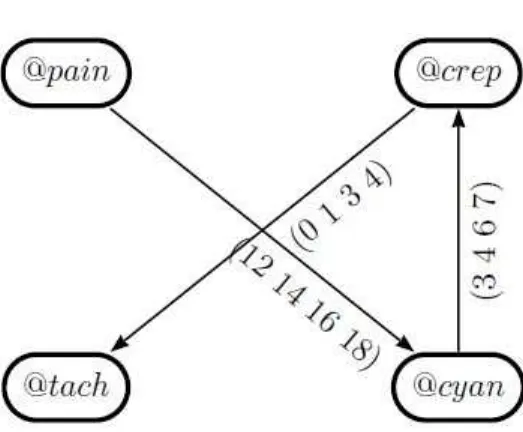
On the other hand, a possible pattern which confirms the Retrograde Car-diac Insufficiency (RCI) hypothesis might be expressed as arule clause:
(rci(present,@rci)∨ ¬pain(present,@pain)∨
¬tachycardia(present,@tach)∨ ¬crepitants(present,@crep)∨ ¬cyanosis(present,@cyan), ρ2)
Figure 2: ρT1 no minimized.
Figure 4: ρ2.
3.2. Resolution Principle in FTCLogic
For the resolution principle for FTCLogic we consider only FTCLogic clauses with the first component in the form of a Horn clause. In other words:
• Fact clauses: (p(...), ρi)
• Rules clauses: (p1(...)∨ ¬p2(...)∨...∨ ¬pn, ρi) • Goal clauses: (¬p1(...)∨ ¬p2(...)∨...∨ ¬pn, ρi)
whereρi is the FTCN associated to eachL-clause.
In the unification process, the formula below will be applied to calculate the resolvent:
((p1(...)∨ ¬p2(...)∨...∨ ¬pn(...)), ρi)
((¬p1(...)∨ ¬pn+1(...)∨...∨ ¬pm(...)),ρj)
whereσ is the MGU (Most General Unifier) andρij is theFTCNnetwork
asso-ciated with the resolvent clause. This network will be the result of minimizing ρi∩ρj.
The resolution process will consist of:
1. To the set of starting clauses C, add the clause that is to be tested, C= (ς, ρU) and call the resulting setC′.
2. Seek a deduction from (⊥, ρmax) by applying the resolution rule
reitera-tively to C′, such that ρ
max will be the maximal network obtained with
each of the ρi networks, such that the (⊥, ρi) has been deduced in the
resolution.
3. Finally, V al(ς,C) will beNN((⊥, ρmax)).
As stated earlier, whenever at least one fact clause is necessary to relate two variables temporally, this will be included as a temporal constraint within aρT network that will be associated with a special clause with a unique literal
calledT ime. In other words: (T ime, ρT)
consists of a positive predicate without arguments and one FTCN that will store true temporal relations.
For these relations to be taken into account in a resolution process, it will be necessary to include in the goal clause a literal of the type¬T ime. We will also see this in the examples below.
Example 10. Continuing with Example 9, we suppose that we need to know if the patient admitted to the ICCU suffered a retrograde cardiac in-sufficiency. The diagnosis system will use the pattern specified in the same example.
When applying the resolution principle the pattern will be considered as a rule and the predicate associated toretrograde cardiac insufficiency must be included as a negative clause, which will also contain the literal ¬T ime, as mentioned above, so that the (T ime, ρT) clause is necessarily unified in the
resolution and, thus, the constraints of the network are updated, i.e.: (¬rci(present,@rci)∨ ¬T ime, ρU)
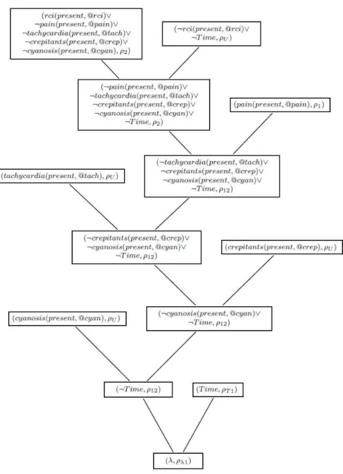
The resolution principle is used to check the consistency of the temporal pattern of Example 9 and the set of manifestations of the same example.
The process of refutation by resolution is summarized in Figure 5.
Figure 6: ρ12.
Figure 3. Elsewhere,ρ12corresponds to the FTCNrepresented in Figure 6 and ρλ1 to that in Figure 7. We avoid all the constraints between the node that signals the start time (0:0:0 hours) and the remaining nodes, since their values would obviously coincide with corresponding ones of @pain.
InFTCLogicthe constraint propagation process is exhaustive, because it is delegated to theFTCNand apath-consistency algorithmthat ensures a minimal network.
4. Description of PROLogic
Figure 7: ρλ1.
4.1. Programs
As inPROLOG, a program is a set of Horn clauses,rules andfacts:
consequent :- antecedent1, antecedent2, ... antecedentN. fact.
The syntax for PROLogic clauses, however, allows the programmer to as-sociate an FTCN with each clause, as in FTCLogic. For example:
consequent :- antecedent ; (n1,n2,(1,2,3,4) minutes), (n1,n3,(2,3,4,5) minutes), (n2,n3,(3,4,5,6) minutes). fact ; (n1,n2,(3,4,5,6) minutes).
The syntax is the following:
<cons> [:- <ant1>, <ant2>, <ant3>, ..., <antN>] [; [(<originNode>, <date>)],
constr1, ...
The second part of the clause, i.e., that which follows the symbol ’;’ specifies an FTCN. If no FTCN appears, the Universal Network will be associated with
PROLogic-clause. In another case, the FTCN will be specified through the
constrXconstraints. constrXcan be given as a fuzzy number or as arelation:
constrX =
(<nodeX1>,<nodeX2>,(<double>,<double>,<double>,<double>), <unit>)
| (<nodeX1>,<nodeX2>,relation)
<unit> can be one of the following words: ‘seconds ’,‘ minutes’, ‘days ’,‘ weeks’, ‘months ’, or ‘years’.
Arelationspecifies a constraint using pseudo-natural language. PROLogic
uses a parser to convert the relations into an equivalent fuzzy number.
PROLogicmakes it possible to instantiate a node of the FTCN, the<originNode>, with a time. To do so, it is necessary to specify it before the constraints. For example:
time ; (node1,(’2016-11-25T12:30:00’, ’2016-11-25T13:00:00’, ’2016-11-25T13:30:00’, ’2016-11-25T14:00:00’)), (node1,node2,(12,14,16,18) minutes).
<originNode>indicates the name of a node that is associated with<date>.
<date>can be a fuzzy date or an absolute date:
<date> = (<dateISO1>,<dateISO2>,<dateISO3>,<dateISO4>) | <dateISO>
<dateISO>indicates a date in ISO 8601 format, i.e., YYYY-MM-DDTHH:MM. An FTCN can have only one node of origin, since more than one assignment is not necessary to determine the rest of the values of the nodes in FTCN. However, it may be the case that during the merging of two networks, they have different, and perhaps incompatible, origin nodes. In this case,PROLogic
keeps the origin of one of the networks and discards the other. The programmer is, therefore, advised to attempt to avoid these cases as much as possible.
If no origin node is specified,PROLogicassigns an unnamed origin node by default, dated 0:00 on January 1 of year 1.
• Multi-line comments. Start with /* and end with */ .
/* Multi-line
comment. */
Example 11. The following PROLogic program encodes the RCI-rule and the facts that are specified in Example 9 as FTCLogic-clauses for a patient named Juan. Other facts are additionally specified for another patient named Manolo:
/* RCI pattern */
rci(present,rci,X) :- pain(present,pain,X), tachycardia(present,tach,X),
crepitants(present,crep,X),
cyanosis(present,cyan,X), time(X) ; (pain,cyan,(-5,-5,40,40) minutes), (pain,crep,(-10,-10,30,30) minutes), (pain,tach,(-15,-15,20,20) minutes), (crep,cyan,(-15,-15,30,30) minutes), (tach,cyan,(-5,-5,35,35) minutes), (tach,crep,(-10,-10,25,25) minutes), (rci,pain,(0,0,20,20) minutes), (rci,cyan,(15,15,40,40) minutes), (rci,crep,(10,10,30,30) minutes), (rci,tach,(5,5,20,20) minutes).
% Facts detected in patient Juan pain(present,pain,juan).
cyanosis(present,cyan,juan). crepitants(present,crep,juan). tachycardia(present,tach,juan).
% the earlier facts
time(juan) ; (pain,(’2016-11-25T12:30:00’, ’2016-11-25T13:00:00’, ’2016-11-25T13:30:00’, ’2016-11-25T14:00:00’)), (pain,cyan,(12,14,16,18) minutes),
(cyan,crep,(3,4,6,7) minutes), (crep,tach,(0,1,3,4) minutes).
% Facts detected in patient Manolo pain(present,pain,manolo).
cyanosis(present,cyan,manolo). crepitants(present,crep,manolo). tachycardia(present,tach,manolo).
% Temporal constraints detected between % the earlier facts
time(manolo) ; (pain,(’2016-11-25T14:30:00’, ’2016-11-25T15:00:00’, ’2016-11-25T15:30:00’, ’2016-11-25T16:00:00’)), (pain,cyan,(10,12,14,16) minutes),
(cyan,crep,(3,4,6,7) minutes), (crep,tach,(0,1,3,4) minutes).
We can see that the time origin0:0:0 of Example 1, has been replaced at the origin given by the fuzzy date(2016-11-25T12:30:00, 2016-11-25T13:00:00, 2016-11-25T13:30:00,
2016-11-25T14:00:00).
4.2. Queries
With the addition of FTCNs, queries become more complex than inPROLOG. That is why, in this case, the classic query interpreter becomes a somewhat more complicated command console, which provides the possibility of accessing many pieces of information related to the networks obtained as a result of a classic query. In this section, we detail the general syntax of a command in the interpreter, and then show, one by one, all the available commands.
more, every <argY>is an argument. At the syntax level, only the name of the command is necessary, but each command may have its own requirements.
The syntax of <goal>is:
<atom1>, <atom2>, ..., <atomN>
Each<FTCN> is described as specified in the previous section. 4.2.1. Load a program
Use:
load <program_file>.
Description:
Load a PROLogic program from a file.
Example 12. We charge the program from Example 11:
?-load ’programRCI.txt’
Program ’programRCI.txt’ correctly loaded.
If the syntax of the program is correct, it indicates that it loads correctly. If there were a lexical or syntactic error, the fault and the line and column in which it was made would be indicated.
4.2.2. Make a query Use:
c [-d|-h|-i] [node1 node2..nodeN] : <goal> [; <FTCN>].
Description:
If the goal FTCN is omitted, the universal network will be used by default. That is, an empty FTCN.
Options:
-d: Defuzzified constraints.
-h: Hide the FTCN in the answer.
-i: This shows the infinite constraints.
Note that in order to simulate a query fromPROLOGthe-h option would be necessary.
Example 13. If we are loading the program as in Example 12, then we can do the following:
?-c : rci(present,rci,x). X = Juan.
Temporal constraints:
(pain,pain,(-5mi,-1mi,1mi,5mi)) (pain,crep,(15mi,18mi,19mi,20mi)) (pain,tach,(15mi,19mi,20mi,20mi)) (pain,rci,(-5mi,-1mi,0sec,0sec)) (pain,cyan,(12mi,14mi,15mi,17mi)) (crep,crep,(-2mi,0sec,0sec,2mi)) (crep,tach,(0sec,1mi,1mi,2mi))
(crep,rci,(-20mi,-19mi,-19mi,-18mi)) (crep,cyan,(-5mi,-4mi,-4mi,-3mi)) (tach,tach,(-2mi,0sec,0sec,2mi)) (tach,rci,(-20mi,-20mi,-20mi,-18mi)) (tach,cyan,(-5mi,-5mi,-5mi,-3mi)) (rci,rci,(-2mi,0sec,0sec,2mi)) (rci,cyan,(15mi,15mi,15mi,17mi)) (cyan,cyan,(-2mi,0sec,0sec,2mi))
Note that the temporal constraints are the same as those of theρλ1 network in Example 10.
We can attain another answer, if any, with the ncommand. Use:
-i: This shows the infinite constraints.
Example 14. We shall use this with the defuzzied network.
?-n -d. X = manolo
Temporal constraints: (pain,pain,0sec) (pain,crep,17mi) (pain,tach,18mi) (pain,rci,-2mi) (pain,cyan,13mi) (crep,crep,0sec) (crep,tach,1mi) (crep,rci,-19mi) (crep,cyan,-4mi) (tach,tach,0sec) (tach,rci,-20mi) (tach,cyan,-5mi) (rci,rci,0sec) (rci,cyan,15mi) (cyan,cyan,0sec)
On the other hand, the commandlastallows us to obtain information about the last answer obtained.
Use:
last [-d|-h|-i] [node1 node2 .. nodeN].
Description:
Returns the current result. Options:
-h: Hide the FTCN in the answer.
-i: This shows the infinite constraints.
This command allows us to modify the options we have used.
Example 15. If we wish to know the fuzzy values of constraints, we can do the following:
?-last. X = manolo
Temporal constraints:
(pain,pain,(-6mi,-2mi,2mi,6mi)) (pain,crep,(13mi,16mi,18mi,20mi)) (pain,tach,(13mi,17mi,19mi,20mi)) (pain,rci,(-7mi,-3mi,-1mi,0sec)) (pain,cyan,(10mi,12mi,14mi,16mi)) (crep,crep,(-2mi,0sec,0sec,2mi)) (crep,tach,(0sec,1mi,1mi,2mi))
(crep,rci,(-20mi,-19mi,-19mi,-18mi)) (crep,cyan,(-5mi,-4mi,-4mi,-3mi)) (tach,tach,(-2mi,0sec,0sec,2mi)) (tach,rci,(-20mi,-20mi,-20mi,-18mi)) (tach,cyan,(-5mi,-5mi,-5mi,-3mi)) (rci,rci,(-2mi,0sec,0sec,2mi)) (rci,cyan,(15mi,15mi,15mi,17mi)) (cyan,cyan,(-2mi,0sec,0sec,2mi))
We could also omit the network:
?-last -h. X = manolo
or focus on the constraints of certain nodes:
?-last pain crep. X = manolo
Temporal constraints:
readable. However, we use the-i option if necessary.
When there are no more answers, the command n warns of this and keeps the last answer in context:
?-n.
There are no more answers. ?-last -h.
X = manolo
4.2.3. Basic information regarding networks
There is a set of commands that makes it possible to obtain additional infor-mation about the network associated with the last answer. These commands may be of interest if we wish to know which event occurred first or last, and which occurred after or before another event.
firsts tells us which nodes occurred before all the others. There may be several.
Use:
firsts.
Description:
Returns the nodes that represent the initial events of the result network. Re-turns more than one if they occurred at approximately the same time.
lasts returns the end nodes in the network. Use:
lasts.
Description:
Returns the nodes that represent the final events of the result network. Returns more than one if they occurred at approximately the same time.
The commandspredandsuccreturn all the nodes that precede and succeed the indicated node, respectively.
Use:
Description:
Returns the nodes that occurred approximately before <node> in the result network.
Use:
succ <node>.
Description:
Returns the nodes that occurred approximately after <node>in the result net-work.
Example 16.
?-n -d. X = manolo
Temporal constraints: (pain,pain,0sec) (pain,crep,17mi) (pain,tach,18mi) (pain,rci,-2mi) (pain,cyan,13mi) (crep,crep,0sec) (crep,tach,1mi) (crep,rci,-19mi) (crep,cyan,-4mi) (tach,tach,0sec) (tach,rci,-20mi) (tach,cyan,-5mi) (rci,rci,0sec) (rci,cyan,15mi) (cyan,cyan,0sec)
?-firsts. rci
?-lasts. tach
time [-d] [<node1>...<nodeN>].
Description:
It returns an absolute time for each node in the answer network, taking into account the origin node of the network, if it exists.
Options:
-d: Defuzzified constraints. Example 17.
?-n -h. X = manolo
?-time.
pain -> (2016-11-25 15:09:00 +0000, 2016-11-25 15:13:00 +0000, 2016-11-25 15:17:00 +0000, 2016-11-25 15:21:00 +0000) crep -> (2016-11-25 15:28:00 +0000, 2016-11-25 15:31:00 +0000, 2016-11-25 15:33:00 +0000, 2016-11-25 15:35:00 +0000) tach -> (2016-11-25 15:28:00 +0000, 2016-11-25 15:32:00 +0000, 2016-11-25 15:34:00 +0000, 2016-11-25 15:35:00 +0000) rci -> (2016-11-25 15:08:00 +0000,
2016-11-25 15:12:00 +0000, 2016-11-25 15:14:00 +0000, 2016-11-25 15:15:00 +0000) cyan -> (2016-11-25 15:25:00 +0000,
We can indicate any origin node with theresolv command. Use:
resolv [-d] <origin_node> <time> [<node1>...<nodeN>].
Description:
It returns an absolute time for each node in the answer network, taking into account the <origin node>argument.
Options:
-d: Defuzzified constraints. Arguments:
<origin node>: node from which the network is resolved.
<time>: time assigned to <origin node>, in ISO-8601 format: YYYY-MM-DDTHH:MM:SS.
Example 18.
?-n -h. X = manolo
?-resolv -d crep ’1999-07-03T16:45:18’. crep -> 1999-07-03 16:45:18 +0000
pain -> 1999-07-03 16:28:18 +0000 tach -> 1999-07-03 16:46:18 +0000 rci -> 1999-07-03 16:26:18 +0000 cyan -> 1999-07-03 16:41:18 +0000
4.2.5. Hypothetical queries
Previous queries allow the extraction of available information. PROLogicallows a second type of queries in order to discover the compatibility between a certain piece of information and the existing one. This can be done using the command
hypo. Use:
hypo <node1> <relation> <node2>.
Description:
<node2>: final node of the constraint.
The possibility degree is a measure between 0 and 1. A 0-value indicates that the relation of the query is impossible, while a 1-value indicates that the relation is totally possible. With respect to necessity degree, it measures the certainty of a relation, signifying that a value greater than 0 would imply a possibility of 1, while a possibility value of 0 would imply a necessity of 0. A necessity value of 0 and a possibility of 1 mean that the relation is completely possible but the certainty is unknown. This implies total ignorance.
Example 19. Let us check, for example, a relationship between thepain
and crepnodes shown in the previous examples.
?-last -d pain crep. X = manolo
Temporal constraints: (pain,pain,0sec) (pain,crep,17mi) (crep,crep,0sec)
?-hypo pain ’approximately 15 minutes before’ crep. Possibility degree: 1.0
Necessity degree: 0.0
The result indicates that the relationship is perfectly possible, although without certainty.
The following relation is, on the other hand, completely incompatible:
?-hypo pain ’approximately 40 minutes before’ crep. Possibility degree: 0.0
Necessity degree: 0.0
4.2.6. Help command
all the commands, with their description and the meaning of their options and arguments. It is the command help.
Use:
help <command1> [<command2>...<comamndN>].
Description:
Describe the use of the commands-arguments. 4.2.7. End session
In order to close the application from the terminal, it is simply necessary to use the command q.
Use:
q.
Description:
The running of the interpreter ends.
5. PROLogic Design
As mentioned previously, PROLogic has been implemented in Haskell. The Alex and Happy tools have also been used as scanner and lexer generators, respectively. They have been used for both the analysis of the programs and the commands interpreter.
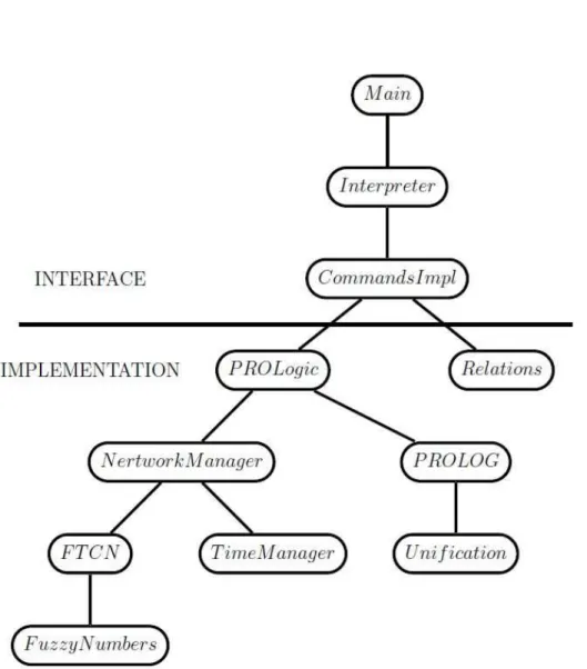
In this section we describe how the different modules interact. Relationships are represented in the hierarchical model that appears in Figure 8. Note that there are two main blocks: interface and implementation.
The interface block contains three main modules: Main, Interpreter and
CommandsImpl. The first is responsible for initializing some of the parameters in the environment and for initiating the commands interpreter. This inter-preter, in turn, executes an interactive and textual interface for the process-ing of different commands: principally loadprocess-ing programs and consultprocess-ing them. The interpreter is responsible only for analyzing the syntax of the commands, through a parser, whose execution passes to the module CommandsImpl. The interpreter and the commands are, therefore, independent.
appropriate functions of the implementation block and write the results. The block consequently also belongs to the interface.
In the implementation block, the main module is PROLogic. The module
Relationsappears at the same level, since both the commands and the programs can include textual temporal relations between two nodes rather than numerical restrictions. This module would be used to perform the translation (through a parser) of that text to numerical restrictions.
The PROLogic module is that which contains the implementation of the FTCLogic resolution process. This process produces a list of answers, consist-ing of a substitution and a network, rather than the list of substitutions that PROLOG would provide. The module also offers some functions with which to perform basic queries on the answers and to obtain additional information about networks or substitutions. This module uses two others: NetworkMan-agerand PROLOG. The first is responsible for managing everything related to networks, thus making the resolution engine and network implementations in-dependent. NetworkManagerensures that the networks included in each clause are always minimized and it is, therefore, always possible to know when we have an inconsistent network. The second contains a basic implementation of PROLOG [1]. In addition, PROLOG uses theUnification module, which con-tains the most basic definitions of logic and allows the calculation of unifiers (substitutions between variables).
The implementation of the main algorithms for network management, such as the minimization and mixing algorithms, is found in theFTCNmodule. The nodes are simple numerical values and the restrictions between them are defined by fuzzy numbers, whose definition and functions are in the FuzzyNumbers
module.
The NetworkManager module also uses the TimeManager module, which contains a series of definitions and functions that allow the use of temporal units in the network constraints. It also allows NetworkManager to assign absolute times to all nodes in the network, starting from the assignment for a particular node.
5.1. Complexity analysis
(access with O(log (n)) in order to reduce the impact of searches. 5.1.1. Query commands
We shall first study the complexity of the command c, after which we shall show those of n and oflast.
Letn be the number of rules in the program, m be the average number of nodes per clause,r be the number of facts in the program,sbe the number of atoms in the goal clause, tbe the number of nodes in the goal network, and k be the average number of atoms in the consequent of a program rule.
Commandc
SincePROLogic is implemented in Haskell, not all the possible answers are calculated, but only the first one, which is that required by the command. This is owing to the lazy evaluation. In the worst case, in order to obtain the answer it is necessary to go completely through the search tree created by PROLogic. The size of this tree is determined by the number of atoms in the goal (s), the number of clauses in the program (n+r) and the number of atoms that have the consequents of the rules (k).
Taking into account the number of times an intersection of two networks must be made, the complexity of this operation, and the minimization that must be carried out at the end, we have calculated an order of complexity of:
O(((n+r)skn +1
−1
k−1 −1)((n+r)m+t)5)
Commandn
The command n places us in a similar situation. The worst possible case is the scenario of having found a first solution in exactly ssteps, and that the next one is at the end of the search tree. This would give us a complexity of
O(((n+r)skn +1
−1
k−1 −1−s)((n+r)m+t)5) Commandlast
Thelastcommand is the simplest of all. It does not calculate any solution, but merely shows the last one obtained. Its complexity is
5.1.2. Basic information commands We assume that the size of the network, measured in nodes, isn.
The complexity of the commandspred and succ is the same, since their implementation varies only in the check that the nodes of the network are located before or after a given one. Both have O(n3).
Furthermore, the complexity of the firstsand lastscommands is O(n4). 5.1.3. Resolution network commands
The commands time and resolv are implemented in a similar way. As in the previous section, we assume that the size of the network isn.
If no specific nodes are requested in these commands, it is assumed that the solution for the entire network is required. The complexity of these commands isO(n3)
5.1.4. Hypothetical query command
Finally, we have analyzed the command hypo, which is quite simple: process the relation, attain the absolute constraint between the nodes and compare it with the relation.
A relation can be a disjunction of subrelations. If r is the number of such subrelations and s is the average number of words in each subrelation, the complexity of this command is
O(n2+rs).
6. Evaluation of PROLogic with an Example: Avian Influenza Probable person-to-person transmission of H5N1
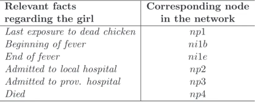
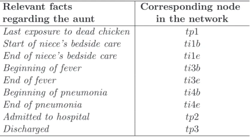
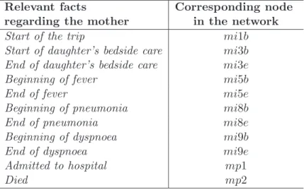
have created a table that will describe the main events related to the disease and its contagion. Each of the entries in the table corresponds to a PROLogic fact. One of the terms of this fact is a node in the FTCN. This network will temporarily relate some facts to others. Table 1 contains the most important events related to the girl while Table 2 shows those of the aunt and Table 3 shows those of the mother. Those events that occur in a time interval have been translated into two events corresponding to the beginning and the end of that interval. This is done in order to enable them to be handled with an FTCN.
Relevant facts Corresponding node
regarding the girl in the network
Last exposure to dead chicken np1
Beginning of fever ni1b
End of fever ni1e
Admitted to local hospital np2
Admitted to prov. hospital np3
Died np4
Table 1: Temporal events associated with the girl.
The objective is to determine whether there is an infection between humans. We achieve this goal by following three steps.
First, we consider the symptoms for each patient, and possible contacts with infected subjects. These are the facts of the program. These facts are related to each other through temporal constraints. Example 20 shows a fragment of a
PROLogic program that specifies the main facts corresponding to the girl, the aunt and the mother. We can also observe the temporal constraints between some of these events. All this is part of a complete PROLogicprogram.
By using the facts contained in the program, and choosing an appropriate time origin, we could, for example, by means of theresolvcommand, assign a date to each event of each patient. This corresponds to obtaining solutions for the network associated with each one of them. That is, by using the command
resolv -d ’origin’ ’2004-09-02T00:00:00’.
Relevant facts Corresponding node
regarding the aunt in the network
Last exposure to dead chicken tp1
Start of niece’s bedside care ti1b
End of niece’s bedside care ti1e
Beginning of fever ti3b
End of fever ti3e
Beginning of pneumonia ti4b
End of pneumonia ti4e
Admitted to hospital tp2
Discharged tp3
Table 2: Temporal events associated with the aunt.
to that specified in [19].
Example 20. Some facts regarding the patients that are part of the pro-gram employed to detect the person-to-person transmission of the H5N1 virus:
exposureChicken(yes,np1,girl). begFever(yes,ni1b,girl).
endFever(yes,ni1e,girl). admLocalHosp(yes,np2,girl). admHosp(yes,np3,girl). died(yes,np4,girl).
time(girl) ;
(origin,(’2004-09-02T00:00:00’,’2004-09-02T00:00:00’, ’2004-09-02T23:59:59’,’2004-09-02T23:59:59’)),
(CP=np1,CF=ni1b, (60,72,96,108) horas),
(CF=ni1b,origin,’approximately equal hours’), (CF=ni1b,FF=ni1e,’before’),
(origin,IHL=np2, ’approximately 5 days before’), (IHL=np2, CF=ni1b, ’after’),
(IHL=np2, FF=ni1e, ’before’),
(IHL=np2,IH=np3, ’approximately 1 day before’), (IH=np3,M=np4, (2,3,3,4) hours).
Beginning of fever mi5b
End of fever mi5e
Beginning of pneumonia mi8b
End of pneumonia mi8e
Beginning of dyspnoea mi9b
End of dyspnoea mi9e
Admitted to hospital mp1
Died mp2
Table 3: Temporal events associated with the mother.
startCare(yes,ti1b,aunt). endCare(yes,ti1e,aunt). begFever(yes,ti3b,aunt). endFever(yes,ti3e,aunt). begPneumonia(yes,ti4b,aunt). endPneumonia(yes,ti4e,aunt). admHosp(yes,tp2,aunt).
discharged(yes,tp3,aunt).
time(aunt) ;
(origin,(’2004-09-02T00:00:00’,’2004-09-02T00:00:00’, ’2004-09-02T23:59:59’,’2004-09-02T23:59:59’)),
(CP=tp1,origin,(3,3,3,3) days),
(CC=ti1b,FC=ti1e, (12,12,13,13) hours),
(origin,CC=ti1b, ’approximately 5 days before’), (origin,CF=ti3b,’approximately 14 days before’), (CF=ti3b,FF=ti3e,’before’),
(CF=ti3b, CN=ti4b,’approximately 7 days before’), (CN=ti4b,FN=ti4e,’before’),
(origin,IH=tp2,(21,21,21,21) days), (CF=ti3b,IH=tp2,’before’),
startTrip(yes,mi1b,mother). startCare(yes,mi3b,mother). endCare(yes,mi3e,mother). begFever(yes,mi5b,mother). endFever(yes,mi5e,mother). begPneumonia(yes,mi8b,mother). endPneumonia(yes,mi8e,mother). begDyspnoea(yes,mi9b,mother). endDyspnoea(yes,mi9e,mother). admHosp(yes,mp1,mother). died(yes,mp2,mother).
time(mother) ;
(origin,(’2004-09-02T00:00:00’,’2004-09-02T00:00:00’, ’2004-09-02T23:59:59’,’2004-09-02T23:59:59’)),
(origin,CVH=mi1b,’approximately 5 days before’), (CC=mi3b, FC=mi3e, (16,16,18,18) hours),
(origin,CF=mi5b, (7,8,9,10) days), (CF=mi5b,FF=mi5e, ’before’),
(origin, IH=mp1,’approximately 15 days before’), (CN=mi8b,IH=mp1,’before’),
(FN=mi8e,IH=mp1,’after’), (CN=mi8b,FN=mi8e,’before’), (CD=mi9b,IH=mp1,’before’), (FD=mi9e,IH=mp1,’after’), (CD=mi9b,FD=mi9e,’before’), (origin,M=mp2,’19 days before’).
time(aunt,mother);
(origin,(’2004-09-02T00:00:00’,’2004-09-02T00:00:00’, ’2004-09-02T23:59:59’,’2004-09-02T23:59:59’)),
(CC=ti1b, CC=mi3b,’before’), (CC=ti1b, FC=mi3e, ’before’), (FC=ti1e, CC=mi3b, ’after’), (FC=ti1e, FC=mi3e, ’before’),
pneumonia. Finally, death occurs between 6 and 30 days after the onset of the disease. This pattern can be represented with the PROLogicrule that appears in Example 21. This rule will be part of the program to which the clauses of Example 20 belong.
Example 21. PROLogic rule that represents the typical pattern of the evolution of a patient with H5N1 virus.
avianInfluenza(yes,GA,X)
:-begFever(yes,CF,X),endFever(yes,FF,X),
begDyspnoea(yes,CD,X),endDyspnoea(yes,FD,X), begPneumonia(yes,CN,X), endPneumonia(yes,FN,X), admHosp(yes,IH,X),died(yes,M,X),
time(X);
(CF,CD,(1,5,5,16) days), (CF,CN,(3,7,7,17) days), (CN,IH,’before’),
(FN,IH,’after’),
(CF,M,(6,6,30,30) days).
Thirdly and finally (Example 22), we could use the complete program to make interesting deductions that would allow us to conclude some aspects re-lated to contagion. In particular, it would be interesting to verify whether this contagion occurred person to person.
Example 22. We summarize the conclusions in the following queries:
• Could the aunt have been infected by the girl? To answer this, we com-pared the time from the end of the care until the beginning of the fever in the aunt, with the standard incubation period (approximately 2 to 10 days). We do this with the following query:
hypo ’FC=ti1e’ ’approximately (2,2,10,10) days before’ ’CF=ti3b’.
In fact, if we check the elapsed time using the command
c ’FC=ti1e’ ’CF=ti3b’: time(aunt).
the result is(5d 11h,1week 11h,1week 2d 12h,1week 4d 12h) (defuzzi-fied: 1week 1d 11h 30mi), that is, approximately 8 days.
• Could the aunt have been infected by the mother? This would be possible if the time of care of the aunt and the mother had overlapped. We consult this with the command:
c ’CC=mi3b’ ’FC=ti1e’: time(aunt,mother),time(aunt), time(mother).
and the result is true: (0sec,0.1sec,12h 59mi 59sec,13h).
• Could the aunt have been infected by the chickens? If the incubation period is considered to be 10 days maximum, the possibility degree is 0 (and necessity = 0):
hypo ’CP=tp1’ ’less than 10 days before’ ’CF=ti3b’.
We calculate the temporal distance with the command:
c ’CP=tp1’ ’CF=ti3b’: time(aunt).
and the result is(2week 3d,2week 3d,2week 3d,2week 3d)
• Finally, there is no contact between the mother and the chickens. Could the mother have been infected by the girl? We checked whether the incubation period (2-17 days) plus the evolution from symptoms to death (6 to 30 days) was compatible with the time that had elapsed since the mother began to care for the daughter until she died. The next query returned a degree of possibility of 1 and a degree of necessity close to 1:
hypo ’CC=mi3b’ ’(8, 11, 20, 47) days before’ ’M=mp2’.
If we consult the time in the network:
c ’CC=mi3b’ ’M=mp2’: time (mother).
the result is(1week 3d 16h, 1week 5d 19h, 2week 21h, 2week 3d).
7. Conclusions
the first answer compatible with the goal, or warns that the response does not exist. However, when following the model ofFTCLogic, all the clauses have an associated temporal network, signifying that the networks are merged during the resolution process through the intersection of those constraints that relate the same nodes. A final network will be part of the answer. In addition, a temporal network, or “goal network”, can be added to a goal clause. This network must be compatible with the answer network.
The interpreter also implements temporal commands and a help command. We have analyzed the computational complexity associated with temporal commands. This must be added to the complexity of the commands of any
PROLOGinterpreter.
We have validated PROLogic with an example of the probable person-to-person transmission of avian influenza [19] with very good results.
PROLogic is currently a proof of concept that should be improved and evaluated until the final application is obtained. In this final application we could consider including reasoning with time intervals by simply translating these intervals into point-to-point relationships to operate in anFTCNnetwork, as occurs in theFuzzyTIME temporal reasoner [4].
Acknowledgements
This work was partially funded by the Spanish Ministry of Science, Innovation and Universities under the SITSUS project (Ref: RTI2018-094832-B-I00), and by the European Fund for Regional Development (EFRD, FEDER).
References [1] J.A. Alonso Jim´enez, L´ogica en Haskell, In:
https://www.cs.us.es/˜jalonso/publicaciones/2007-Logica en Haskell.pdf (2007), 113-134.
[3] P. Blackburn, J. Bos and K. Striegnitz, Prolog Syntax, In: http://www.learnprolognow.org/lpnpage.php?pagetype=html
&pageid=lpn-htmlse2 (2012).
[4] M. Campos, J.M. Juarez, J. Palma, R. Marn, and F. Palacios, Avian Influenza: Temporal modeling of a human to human transmission case,
Expert Systems with Applications, 38(2011), 8865-8885.
[5] M.A. C´ardenas-Viedma and R. Mar´ın, FTCLogic: Fuzzy temporal constraint logic, Fuzzy Set and Systems, 363 (2019), 84-112; DOI: 10.1016/j.fss.2018.05.014.
[6] R. Dechter, I. Meiri and J. Pearl, Temporal constraint networks, Artificial Intelligence,49(1991), 61-65.
[7] D. Dubois and H. Prade, Processing fuzzy temporal knowledge, IEEE Trans. on Systems, Man and Cybernetics,19, No 4 (1989), 729-744. [8] D. Dubois and H. Prade, Possibility tTheory and its applications: Where
do we stand?, In: Springer Handbook Computational Intelligence, Eds. Janusz Kacprzuk and Witold Pedrycz (2015), 31-60, Springer Berlin Hei-delberg.
[9] D. Dubois and H. Prade, Possibilistic logic - An overview, In: Handbook of the History of Logic. Volume 9: Computational Logic. J. Siekmann, Vol. Eds.; D.M. Gabbay, J. Woods, Series Eds. (2015), 283-342.
[10] S. Dutta, A Temporal Logic for uncertain events and an outline of a pos-sible implementation in an extension of PROLOG, Proc.s of the Fourth Conf. on Uncertainty in Artificial Intelligence, UAI (1988).
[11] F.M. Galindo-Navarro and M.A. C´ardenas-Viedma,PROLogic, In: https://webs.um.es/mariancv/PROLogic/PROLogic.exe (2017).
[12] A. Kaufmann and M. Gupta, Introduction to Fuzzy Arithmetic, Van Nos-trand Reinhold, New York (1985).
[13] R. Marn, M.A. C´ardenas-Viedma, M. Balsa and J.L. S´anchez, Obtaining solutions in fuzzy constraint networks,Intern. J. of Approximate Reason-ing16, No 3-4 (1997), 261-288.
[14] S. Marlow,Happy User Guide. In:
[17] E. Lamma, M. Milano and P. Mello, Extending constraint logic program-ming for temporal reasoning, Annals of Math. and Artificial Intelligence, 22, No 1-2 (1998), 139-158.
[18] E. Schwalb and L. Vila, Logic programming with temporal constraints,
Proc. Third Intern. Workshop on Temporal Representation and Reasoning (TIME ’96), Key West, FL - USA (1996), 51-56.