Transmuted Weibull Distribution: A Generalization of theWeibull Probability Distribution

(1)

EUROPEAN JOURNAL OF PURE AND APPLIED MATHEMATICS Vol. 4, No. 2, 2011, 89-102

ISSN 1307-5543 – www.ejpam.com

Transmuted Weibull Distribution: A Generalization of the Weibull

Probability Distribution

Gokarna R. Aryal

1,∗

_{, Chris P. Tsokos}

2

1_{Department of Mathematics, Computer Science and Statistics,}

Purdue University Calumet, Hammond, IN 46323 USA

2_{Department of mathematics and Statistics,}

University of South Florida,Tampa, FL 33620 USA

Abstract. In this article, the two parameter Weibull probability distribution is embedded in a larger

family obtained by introducing an additional parameter. We generalize the two parameter Weibull distribution using the quadratic rank transmutation map studied by Shawet al.[9]to develop a trans-muted Weibull distribution. We provide a comprehensive description of the mathematical properties of the subject distribution along with its reliability behavior. The usefulness of the transmuted Weibull distribution for modeling reliability data is illustrated using real data.

2000 Mathematics Subject Classifications: 62N05; 90B25

Key Words and Phrases: Weibull distribution, hazard rate function, reliability function, parameter

estimation

1. Introduction

The quality of the procedures used in a statistical analysis depends heavily on the assumed probability model or distributions. Because of this, considerable effort has been expended in the development of large classes of standard probability distributions along with revelent sta-tistical methodologies. However, there still remain many important problems where the real data does not follow any of the classical or standard probability models.

The Weibull distribution is a very popular distribution named after Waladdi Weibull, a Swedish physicist. He applied this distribution in 1939 to analyze the breaking strength of materials. Since then, it has been widely used for analyzing lifetime data in reliability engineering. It is a versatile distribution that can take on the characteristics of other types of distributions, based on the value of the shape parameter. The Weibull distribution is a widely used sta-tistical model for studying fatigue and endurance life in engineering devices and materials.

∗_{Corresponding author.}

Email addresses:aryalgpurdueal.edu(G. Aryal),profptas.usf.edu(C. Tsokos)

(2)

G. Aryal, C. Tsokos Eur. J. Pure Appl. Math,4(2011), 89-102 90

Many examples can be found among the aerospace, electronics, materials, and automotive in-dustries. Recent advances in Weibull theory have also created numerous specialized Weibull applications. Modern computing technology has made many of these techniques accessible across the engineering spectrum. Despite its popularity, and wide applicability the traditional 2-parameter and 3-parameter Weibull distribution is unable to capture all the lifetime phe-nomenon for instance the data set which has a non-monotonic failure rate function. Recently several generalization of Weibull distribution has been studied. An approach to the construc-tion of flexible parametric models is to embed appropriate competing models into a larger model by adding shape parameter. Some recent generalizations of Weibull distribution includ-ing the exponentiated Weibull, extended Weibull, modified Weibull are discussed in Phamet al.[7]and references therein, along with their reliability functions. In this article we present a new generalization of Weibull distribution called the transmuted Weibull distribution. We will derive the subject distribution using the quadratic rank transmutation map studied by

Shawet al. [9].

A random variable X is said to have transmuted distribution if its cumulative distribution function(cdf) is given by

F(x) = (1+λ)G(x)−λG(x)2, |λ| ≤1 (1)

whereG(x)is the cdf of the base distribution. Observe that atλ=0 we have the distribution of the base random variable. Aryal et al. [1]studied the the transmuted Gumbel distribu-tion and it has been observed that transmuted Gumbel distribudistribu-tion can be used to model climate data. In the present study we will provide mathematical formulation of the trans-muted Weibull distribution and some of its properties. We will also provide possible area of applications.

2. Transmuted Weibull Distribution

A random variable X is said to have a Weibull distribution with parameters η > 0 and σ >0 if its probability density function (pdf) is given by

g(x) = η

σ x

σ η−1

exp

−x

σ η

x >0 (2)

The cdf ofX is given by

G(x) =1−exp

−x

σ η

. (3)

Now using (1) and (3) we have the cdf of a transmuted Weibull distribution

F(x) =

1−exp

−x

σ

η

1+λexp

−x

σ η

. (4)

Hence, the pdf of transmuted Weibull distribution with parametersη,σandλis

f(x) = η

σ x

σ η−1

exp

−x

σ η

1−λ+2λexp

−x

σ η

(3)

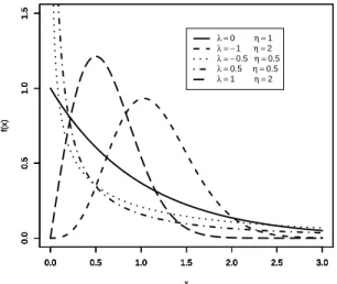
Note that the transmuted Weibull distribution is an extended model to analyze more complex data and it generalizes some of the widely used distributions. In particular for η = 1 we have the transmuted exponential distribution as discussed in Shaw et al.[9]. The Weibull distribution is clearly a special case forλ=0. Whenη=λ=1 then the resulting distribution is an exponential distribution with parameter σ₂. Figure 1 illustrates some of the possible shapes of the pdf of a transmuted Weibull distribution for selected values of the parametersλ andηand forσ=1.

0.0 0.5 1.0 1.5 2.0 2.5 3.0

0.0

0.5

1.0

1.5

x

f(x)

0.0 0.5 1.0 1.5 2.0 2.5 3.0

0.0

0.5

1.0

1.5

0.0 0.5 1.0 1.5 2.0 2.5 3.0

0.0

0.5

1.0

1.5

0.0 0.5 1.0 1.5 2.0 2.5 3.0

0.0

0.5

1.0

1.5

0.0 0.5 1.0 1.5 2.0 2.5 3.0

0.0

0.5

1.0

1.5

x

f(x)

λ =0 η =1

λ = −1 η =2

λ = −0.5 η =0.5

λ =0.5 η =0.5

λ =1 η =2

Figure1: pdfoftransmutedWeibulldistributionforσ=1anddierentvaluesofλ andη

3. Moments and Quantiles

In this section we shall present the moments and qunatiles for the transmuted Weibull distribution. Thekthorder moments of a transmuted Weibull random variableX, in terms of gamma functionΓ(.), is given by

E(Xk) =σkΓ

1+ k

η §

1−λ+λ2−

k

η

ª

(6)

Moreover, ifk/η=r is a positive integer, then

E(Xk) =σkr!1−λ+λ2−r

Therefore, the expected value E(X) and variance Var(X) of a transmuted Weibull random variable X are, respectively, given by

E(X) = σΓ

1+ 1

η

1−λ+λ2−1η

(4)

Var(X) = σ2

Γ

1+ 2

η

1−λ+λ2−

2 η

−Γ2

1+ 1

η

1−λ+λ2−

1 η

2 .

Note that whenη=k,

E(Xk) =σk

₂−_λ 2

.

Theqthquantile x_qof the transmuted Weibull distribution can be obtained from (4) as

xq=σ

     −ln    1−  

1+λ−p(1+λ)2₋_4λ_q

2λ           1/η (7)

In particular, the distribution median is

x_0.5=σ



 −ln



 

λ−1+p1+λ2

2λ       1/η .

3.1. Random Number Generation and Parameter Estimation

Using the method of inversion we can generate random numbers from the transmuted Weibull distribution as

1−exp

−x

σ η

(1−λ) +λexp

−x

σ η

=u

whereu∼U(0, 1). After simple calculation this yields

x=σ

     −ln    1−  

1+λ−p(1+λ)2₋_4λ_u

2λ           1/η . (8)

One can use equation (8) to generate random numbers when the parametersη,σandλ are known. The maximum likelihood estimates, MLEs, of the parameters that are inherent within the transmuted Weibull probability distribution function is given by the following:

Let X₁,X₂,· · ·,X_n be a sample of size nfrom a transmuted Weibull distribution. Then the

likelihood function is given by

L= η σ n exp  − n X

i=1

_x i σ η   n Y

i=1

_x

i

σ η−1

×1−λ+2λexp

−xi

σ η

.

Hence, the log-likelihood functionL =lnLbecomes

L = nlnη

σ−

n

X

i=1

_x i σ η + n X

i=1

ln _x

i

σ η−1

+

n

X

i=1

ln

1−λ+2λexp

−xi

(5)

= nlnη−nηlnσ+ (η−1)

n

X

i=1

ln(x_i)−

n

X

i=1

_x i σ η + n X

i=1

ln

1−λ+2λexp

−xi

σ η

. (9)

Therefore, the MLEs of η,σ and λ which maximize (9) must satisfy the following normal equations

∂L ∂ η =

n

η+

n

X

i=1

1−

x

i

σ η

ln x i σ −2λ n X

i=1

ln(x_i/σ)(x_i/σ)ηexp(−(x_i/σ)η)

1−λ+2λexp(−(xi/σ)η)

=0,

∂L

∂ σ = − η σ

n

X

i=1

1−xi

σ η

+2λη

σ

n

X

i=1

(x_i/σ)η_exp₍₋₍_x

i/σ)η)

1−λ+2λexp(−(x_i/σ)η₎ =0, ∂L

∂ λ =

n

X

i=1

2 exp(−(xi/σ)η)−1

1−λ+2λexp(−(x_i/σ)η) =0.

The maximum likelihood estimatorθˆ=η,ˆ σ,ˆ λˆ ′

ofθ = η,σ,λ′

is obtained by solving this nonlinear system of equations. It is usually more convenient to use nonlinear optimization algorithms such as quasi-Newton algorithm to numerically maximize the log-likelihood func-tion given in (9). In order to compute the standard error and asymptotic confidence interval we use the usual large sample approximation in which the maximum likelihood estimators of

θ _{can be treated as being approximately trivariate normal. Hence as}_n→ ∞_{, the asymptotic}

distribution of the MLEη,ˆ σ,ˆ λˆis given by, see Zaindinet al.[10],    ˆ η ˆ σ ˆ λ   ∼N

      η σ λ   ,    ˆ

V11 Vˆ12 Vˆ13

ˆ

V21 Vˆ22 Vˆ23

ˆ

V₃₁ Vˆ₃₂ Vˆ₃₃

      (10)

where,Vˆ_{i j}=V_{i j}|θ=ˆθ and



 

V11 V12 V13

V21 V22 V23

V₃₁ V₃₂ V₃₃

  =   

A11 A12 A13

A21 A22 A23

A₃₁ A₃₂ A₃₃



 

−1

is the approximate variance covariance matrix with its elements obtained from

A₁₁=−∂

2_L

∂ η2 , A12=−

∂2L

∂ η∂ σ,

A₂₂=−∂

2_L

∂ σ2, A23=−

∂2_L

∂ σ∂ λ,

A33=−

∂2L

∂ λ2 , A13=−

∂2L ∂ η∂ λ.

whereL is the log-likelihood function given in (9). An Approximate 100(1−α)% two sided confidence intervals forη,σandλare, respectively, given by

ˆ

η±zα/2

p

ˆ

V11, σˆ±zα/2

p

ˆ

V22andλˆ±zα/2

p

ˆ

(6)

wherezα is the upperα−thpercentiles of the standard normal distribution. For details see

[3, 10]etc.. Using R[2]we can easily compute the Hessian matrix and its inverse and hence the values of the standard error and asymptotic confidence intervals.

4. Reliability Analysis

The transmuted Weibull distribution can be a useful characterization of failure time of a given system because of the analytical structure. The reliability functionR(t), which is the probability of an item not failing prior to some time t, is defined by R(t) = 1−F(t). The reliability function of a transmuted Weibull distribution is given by

R(t) =exp

−t

σ η

1−λ+λexp

−t

σ η

. (11)

The other characteristic of interest of a random variable is the hazard rate function defined by

h(t) = f(t)

1−F(t)

which is an important quantity characterizing life phenomenon. It can be loosely interpreted as the conditional probability of failure, given it has survived to the time t. The hazard rate function for a transmuted Weibull random variable is given by

h(t) = η

σ _t

σ η−1







1−λ+2λexp−_t

σ

η

1−λ+λexp−_t

σ

η 





. (12)

Theorem 1. The hazard rate function of a transmuted Weibull distribution has the following properties:

(i) Ifη=λ=1, the failure rate is constant.

(ii) Ifλ=1, then the failure rate is increasing forη >1and decreasing forη <1

(iii) Ifη=1then the failure rate is increasing ifλ <0and is decreasing ifλ >0.

(iv) Ifλ=0andη=1the the failure rate is a constant.

Proof.

(i) Ifλ=η=1 then

h(t) = 2

(7)

(ii) Ifλ=1, then

h(t) = 2η

σ t

σ η−1

.

which is increasing forη >1 and is decreasing forη <1.

Note that forη=2 we have linear hazard function as in the case of Rayleigh distribu-tion.

(iii) Ifη=1 then we have

h(t) = 1

σ+ λ σ

exp(−t/σ)

[1−λ+λexp(−t/σ)].

It can be easily shown thath(t)is increasing forλ <0 and is decreasing forλ >0. Note that

h(0) = 1+λ

σ andh(∞) = 1 σ.

It is clear that that the hazard rate function increases from 0 to _σ1 for λ < 0 and it decreases from _σ2 to_σ1 forλ >0.

(iv) If λ = 0 and η = 1 the the failure rate is a constant as the resulting distribution is exponential distribution.

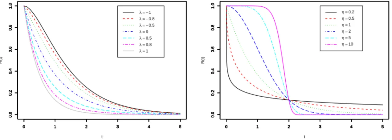
Figure 2 illustrates the reliability behavior of a transmuted Weibull distribution as the value of the parameter λ varies from −1 to 1. Note that the figure on the left shows how

0 1 2 3 4 5

0.0 0.2 0.4 0.6 0.8 1.0 t R(t)

0 1 2 3 4 5

0.0 0.2 0.4 0.6 0.8 1.0

0 1 2 3 4 5

0.0 0.2 0.4 0.6 0.8 1.0

0 1 2 3 4 5

0.0 0.2 0.4 0.6 0.8 1.0

0 1 2 3 4 5

0.0 0.2 0.4 0.6 0.8 1.0

0 1 2 3 4 5

0.0 0.2 0.4 0.6 0.8 1.0

0 1 2 3 4 5

0.0 0.2 0.4 0.6 0.8 1.0

λ = −1

λ = −0.8

λ = −0.5

λ =0

λ =0.5

λ =0.8

λ =1

0 1 2 3 4 5

0.0 0.2 0.4 0.6 0.8 1.0 t R(t)

0 1 2 3 4 5

0.0 0.2 0.4 0.6 0.8 1.0

0 1 2 3 4 5

0.0 0.2 0.4 0.6 0.8 1.0

0 1 2 3 4 5

0.0 0.2 0.4 0.6 0.8 1.0

0 1 2 3 4 5

0.0 0.2 0.4 0.6 0.8 1.0

0 1 2 3 4 5

0.0 0.2 0.4 0.6 0.8 1.0

η =0.2

η =0.5

η =1

η =2

η =5

η =10

Figure2: ReliabilityFuntionofTransmutedWeibullDistribution

(8)

exp(−2)which is independent ofη.

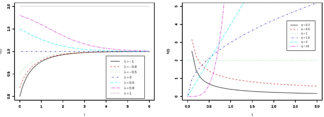
Figure 3 illustrates the behavior of the hazard rate function of a transmuted Weibull distri-bution. Note that the figure on the left shows how the hazard rate function changes its shape when we vary the parameter λ keepingη = 1 andσ = 1 whereas the figure on the right exhibits the behavior as the value ofηchanges keepingλ=1 andσ=1. Observing the

be-0 1 2 3 4 5 6

0.0 0.5 1.0 1.5 2.0 t h(t)

0 1 2 3 4 5 6

0.0

0.5

1.0

1.5

2.0

0 1 2 3 4 5 6

0.0

0.5

1.0

1.5

2.0

0 1 2 3 4 5 6

0.0

0.5

1.0

1.5

2.0

0 1 2 3 4 5 6

0.0

0.5

1.0

1.5

2.0

0 1 2 3 4 5 6

0.0

0.5

1.0

1.5

2.0

0 1 2 3 4 5 6

0.0

0.5

1.0

1.5

2.0

λ = −1

λ = −0.8

λ = −0.5

λ =0

λ =0.5

λ =0.8

λ =1

0.0 0.5 1.0 1.5 2.0 2.5 3.0

0 1 2 3 4 5 t h(t)

0.0 0.5 1.0 1.5 2.0 2.5 3.0

0 1 2 3 4 5 t h(t)

0.0 0.5 1.0 1.5 2.0 2.5 3.0

0 1 2 3 4 5

0.0 0.5 1.0 1.5 2.0 2.5 3.0

0 1 2 3 4 5

0.0 0.5 1.0 1.5 2.0 2.5 3.0

0 1 2 3 4 5

0.0 0.5 1.0 1.5 2.0 2.5 3.0

0 1 2 3 4 5

η =0.2

η =0.5

η =1

η =1.5

η =2

η =10

Figure3: ReliabilityFuntionofTransmutedWeibullDistribution

havior of the hazard rate function it is worth noting that the transmuted Weibull distribution probably will have more applicability than other generalization of the Weibull distribution.

Many generalized Weibull models have been proposed in reliability literature through the fundamental relationship between the reliability functionR(t)and its cumulative hazard rate functionH(t)given byH(t) =−lnR(t). The cumulative hazard rate function of a transmuted Weibull random variable is given by

H(t) =

Z t

0

h(x)d x=

t

σ η

−ln

1−λ+λexp

−t

σ η

.

Observe that:

(i) H(t)is nondecreasing for allt≥0, (ii) H(0) =0,

(iii) lim_t_→∞H(t) =∞.

Given that a unit is of aget, the remaining time after timet is random. The expected value of this random residual life is called the mean residual life(MRL) at time t. The mean residual life (MRL) at a given timetmeasures the expected remaining life time of an individual of age

t. It is given by

(9)

= 1

R(t)

Z ∞

t

R(u)du

Note thatm(0)is the mean time to failure. The MRL can be expressed in terms of the cumu-lative hazard rate function as

m(t) =

Z ∞

0

exp[H(t)−H(t+x)]d x.

The mean residual life can also be related to the failure rate h(t) of the random variable throughm′(t) =m(t)h(t)−1.

The MRL function as well as the hazard rate or failure rate(FR) function is very important as each of them can be used to characterize a unique corresponding life time distribution. Life times can exhibit IMRL (increasing MRL) or DMRL (decreasing MRL). MRL functions that first decreases (increases) and then increases (decreases) are usually called bathtub (upside-down bathtub) shaped, BMRL (UMRL). The relationship between the behaviors of the two functions of a distribution was studied by many authors. The following theorem in[4]summarizes the results of the studies.

For a nonnegative random variable T with pdf f(t), finite meanµ, and differentiable FR functionh(t), the MRL function is

(i) Constant=µif T has an exponential distribution. (ii) DMRL (IMRL) ifh(t)) is IFR (DFR).

(iii) UMRL (BMRL) with a unique change pointt_mifh(t)is BFR (UFR) with a unique change pointt_r, 0<t_m<t_r<∞and f(0)µ >1(<1).

In industrial reliability studies of repair, replacement and other maintenance strategies, the mean residual life function may be proven to be more relevant than the failure rate function. If the goal is to improve the average system lifetime then the mean residual life is the relevant measure. Note that the failure rate function relates only to the risk of immediate failure where as the mean residual life summaries the entire residual life distribution.

The MRL functionm(t)for a transmuted Weibull random variable can be expressed in terms of incomplete Gamma function as given below:

m(t) =σ

η

exp(_σt)η

[1−λ+λexp−(_σt)η

]

(1−λ)Γ

₁ η,

_t

σ η

+λ2−

1 η_Γ

₁ η, 2

_t

σ η

,

whereΓ(a,x) =R∞

x e

(10)

5. Order Statistics

We know that ifX₍₁₎,X₍₂₎,· · ·,X₍_n₎denotes the order statistics of a random sample

X₁,X₂,· · ·,X_nfrom a continuous population with cdfF_X(x)and pdf f_X(x)then the pdf ofX₍_j₎

is given by

f_X(j)(x) = n!

(j−1)!(n−j)!fX(x)[FX(x)]

j−1_[₁₋_F

X(x)]n−j

for j=1, 2,· · ·,n.

We have from (2) and (3) the pdf of the jthorder Weibull random variableX(j)given by

g_X(_j)(x) = n!

(j−1)!(n−j)!

η σ

x

σ η−1

exp

−(n+1− j)

x

σ η

1−exp

−x

σ

ηj−1

Therefore, the pdf of thenthorder Weibull statisticX₍_n₎is given by

g_X(n)(x) = nη

σ _x

σ η−1

exp

−x

σ η

1−exp

−x

σ

ηn−1

(13)

and the pdf of the 1s t order Weibull statisticX(1)is given by

gX(1)(x) =

nη

σ x

σ η−1

exp

−nx

σ η

(14)

Note that in a particular case ofn=2, (13) yields

g_X(₂₎(x) = 2η

σ _x

σ η−1

exp

−x

σ η

1−exp

−x

σ η

(15)

and (14) yields

gX(1)(x) =

2η σ

x

σ η−1

exp

−2

x

σ η

(16)

Observe that (15) and (16) are special cases of (5) forλ=−1 andλ=1 respectively. Theo-rem below summarizes this relationship.

Theorem 2. Suppose we have a system containing two components with each of them having independent and identical Weibull distribution. If the components are connected in series then the

overall system will have transmuted Weibull distribution withλ=1whereas if the components

are parallel then the overall system will have transmuted Weibull distribution withλ=−1.

(11)

Examples of systems with components in parallel include automobile headlights, RAID com-puter disk array system, stairwells with emergency lightings, overhead projectors with backup bulbs etc.

It has been observed that a transmuted Weibull distribution with λ = 1 is the distribution of min(X₁,X₂) and a transmuted Weibull distribution with λ = −1 is the distribution of the ma x(X₁,X₂) where X₁ and X₂ are independent and identically distributed 2-parameter Weibull random variables.

Now we provide the distribution of the order statistics for transmuted Weibull random vari-able. The pdf of the jthorder statistic for transmuted Weibull distribution is given by

f_X(_j)(x) = n!

(j−1)!(n− j)!

η σy

η−1

η _exp₍−_y₎₁−_λ₊_2λ_exp −_y ₁₊_λ_exp −_yj−1

×

1−exp −yj−1exp

−(n−j)y 1−λ+λexp −yn−j,

where,

y =

_x

σ η

Therefore, the pdf of the largest order statisticX(n)is given by

f_X(n)(x) = nη

σ _x

σ η−1

exp

−x

σ η

1−λ+2λexp

−x

σ η

×1+λexp

−x

σ

ηn−1 1−exp

−x

σ

ηn−1

and the pdf of the smallest order statisticX(1)is given by

fX(1)(x) =

nη

σ x

σ η−1

exp

−x

σ η

1−λ+2λexp

−x

σ η

×exp

−x

σ η §

1−λ+λexp

−x

σ

ªn−1 .

Note thatλ=0 yields the order statistics of the two parameter Weibull distribution.

6. Applications of Transmuted Weibull Distribution

In this section we will study two real data sets to illustrate the usefulness of the transmuted Weibull distribution for modeling reliability data. We will make comparison of the results with the exponentiated Weibull distribution whose cdf is given by

F(x) =

1−exp

−x

σ γα

, x >0,α,σ,γ >0 (17)

(12)

consists of 100 centimeter yarn sample at 2.3 percent strain level. This data was studied by Quesenberryet al. [8]. The Weibull distribution (2) is fitted to the subject data and the pa-rameter estimates computed are given in the table below. We fitted both the exponentiated Weibull and transmuted Weibull distribution to the subject data. The MLEs and the values of maximized log-likelihoods for Weibull, exponentiated Weibull and transmuted Weibull distri-bution are given in the table below. One can use the likelihood ratio test to show that the

Table1: EstimatedParametersofWeibull,ExponentiatedWeibullandTransmutedWeibullDistributions

Distribution Parameter Estimates Log-likelihood

Weibull ηˆ=1.60,σˆ=247.9 -627.0500

Exp.Weibull αˆ=1.000001588,σˆ=243.541641,γˆ=1.500001745 -625.5765 Tran. Weibull ηˆ=1.7187616,σˆ =330.2877498,ˆλ=0.7502233 -624.5224

transmuted Weibull distribution fits the subject data better than the 2-parameter Weibull and exponentiated Weibull distribution. Furthermore, the graphical comparison corresponding to these fits to conform our claim is illustrated in figure 4. The second data set is the breaking

0 200 400 600 800

0.0

0.2

0.4

0.6

0.8

1.0

x

F(x)

0 200 400 600 800

0.0

0.2

0.4

0.6

0.8

1.0

x

F(x)

0 200 400 600 800

0.0

0.2

0.4

0.6

0.8

1.0

x

F(x)

0 200 400 600 800

0.0

0.2

0.4

0.6

0.8

1.0

x

F(x)

Empirical Transmuted_Weibull Weibull Exponentiated_Weibull

Figure4: Empirial,FittedWeibull,ExponentiatedWeibullandTransmutedWeibullCDFofWarpBreakage Data

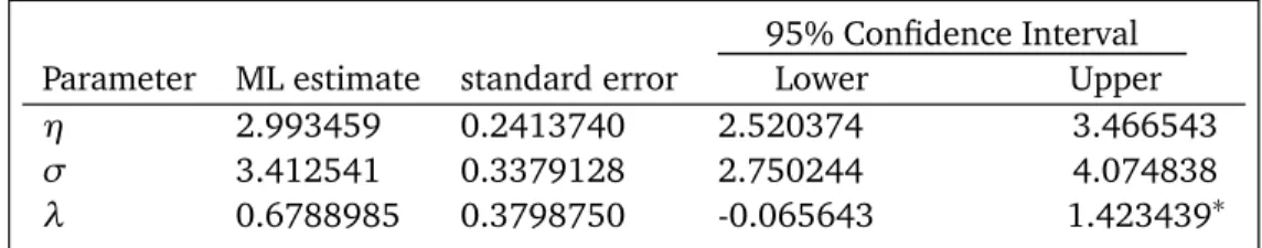
stress of carbon fibers. The data set contains 100 observations on breaking stress of carbon fibers (in Gba) studied by Nichols and Padgett[5]and discussed in[6]to show the usefulness of exponentiated Weibull distribution (17). It is shown (in[6]) that the subject data fits well the exponentiated Weibull distribution with its MLEs and the maximized log-likelihood given by

ˆ

α=1.17262,σˆ=2.79673,γˆ=2.57902 and − L =141.369

(13)

Table2: EstimatedParametersoftheTransmutedWeibullDistributionforBreakingStressData

95% Confidence Interval Parameter ML estimate standard error Lower Upper

η 2.993459 0.2413740 2.520374 3.466543

σ 3.412541 0.3379128 2.750244 4.074838

λ 0.6788985 0.3798750 -0.065643 1.423439∗

the transmuted Weibull distribution−L =141.1349.

This shows that the transmuted Weibull distribution fits equally well the subject data. More-over, we can perform the graphical comparison such as probability plots (not shown here) corresponding to these fits to conform our claim. From these examples it can be observed that transmuted Weibull distribution can be a good competitor of other generalized Weibull distributions to model the reliability data.

7. Concluding Remarks

In the present study, we have introduced a new generalization of the Weibull distribution called the transmuted Weibull distribution. The subject distribution is generated by using the quadratic rank transmutation map and taking the 2-parameter Weibull distribution as the base distribution. Some mathematical properties along with estimation issues are addressed. The hazard rate function and reliability behavior of the transmuted Weibull distribution shows that the subject distribution can be used to model reliability data. We have studied two data sets published in the literature to show the usefulness of the transmuted Weibull distribution and to make comparison with exponentiated Weibull distribution. We expect that this study will serve as a reference and help to advance future research in this area.

References

[1] Gokarna R. Aryal and Chris P. Tsokos. On the transmuted extreme value distribution with application. Nonlinear Analysis: Theory, Methods and Applications, 71:1401–1407, 2009.

[2] R. Ihaka and R. Gentleman. R: A language for data analysis and graphics. Journal of

Computational and Graphical Statistics, 5:299–314, 1996.

[3] Govinda Mudholkar, Deo Srivastava, and George Kollia. A generalization of the weibull distribution with application to the analysis of survival data. Journal of the American

Statistical Association, 91(436):1575–1583, 1996.

[4] Manal M. Nassar and Fathy H. Eissa. On the Exponentiated Weibull Distribution.

Com-munications in Statistics - Theory and Methods, 32(7):1317–1336, 2003.

(14)

[5] M. D. Nichols and W.J. Padgett. A bootstrap control chart for Weibull percentiles.Quality

and Reliability Engineering International, 22:141–151, 2006.

[6] M. Pal, M. M. Ali, and J. Woo. On the exponentiated weibull distribution. Statistica., (2):139–147, 2006.

[7] Hoang Pham and Chin-Diew Lai. On Recent Generalizations of the Weibull Distribution.

IEEE Transactions on RELIABILITY, 56(3):454–458, 2007.

[8] C. P. Quesenberry and Jacqueline Kent. Selecting Among Probability Distributions Used in Reliability. Technometrics, 24(1):59–65, 1982.

[9] W. Shaw and I. Buckley. The alchemy of probability distributions: beyond Gram-Charlier expansions, and a skew-kurtotic-normal distribution from a rank transmutation map.. Research report, 2007.