Stabilization of Nonholonomic Robot
Formations: A First-state Contractive
Model Predictive Control Approach
Feng Xie
1and Rafael Fierro
21School of Electrical and Computer Engineering, Oklahoma State University, Stillwater, USA
2MARHES Lab, Department of Electrical and Computer Engineering, University of New Mexico, Albuquerque, USA
A model predictive control algorithm is developed for stabilizing a team of nonholonomic mobile robots navigating in formation within an obstacle-populated environment. In this scenario, the leader robot may need to execute abrupt maneuvers (i.e., sudden stops and backward motions) in order to avoid collisions and accomplish mission objectives. Moreover,follower robots should be capable of tracking their leaders and maintaining desired relative distance and orientation. To this end, nonholonomic trajectory tracking and point stabilization should be combined in a suitable way. Most proposed control algorithms for nonholonomic robots do not have simultaneous tracking and point stabilization capability; therefore, they may perform poorly when the leader robot executes aggressive maneuvers. In this paper, we address this problem by applying model predictive control(MPC). Motivated by thecontractive MPC scheme developed in[14], the proposed algorithm guarantees its stability by adding a contractive constraint on the first state at the beginning of the prediction hori-zon. The resulting MPC scheme is denoted asfirst-state contractive MPC (FSC-MPC). Simulation results are provided to verify the effectiveness of the method.
Keywords: nonholonomic mobile robots, model predic-tive control, formation control, trajectory tracking, point stabilization
1. Introduction
Cooperative decision and control of mobile robot teams have been of great interest in civilian and military applications, as these teams are ex-pected to be capable of performing many key roles in future civilian or battlefield missions. A lot of effort has been put into this area and the use of mobile robots is likely to increase rapidly in the near future. Applications for co-operative control of multi-robot systems include
[31, 12]: Formation control, cooperative clas-sification and surveillance, cooperative attack and rendezvous, environmental sampling, intel-ligent highways, and air traffic control.
Formation control was inspired by the emer-gent self-organization observed in nature, like flocking birds and schooling fish. Each animal in a herd benefits by maximizing the chance of finding food and minimizing its encounters with predators. Teams of UAVs moving in forma-tions with precisely defined geometries lead to many advantages, such as energy saving when the vortex forces are taken into account. Sev-eral experimental studies have verified the en-ergy saved when flying in close formations[37]. In addition, formation control allows for intelli-gentleadersand single agent planning while
fol-lowerscan focus on other tasks. The challenge
here lies in designing a formation controller that is computationally simple, yet robust.
Leader-following is a common approach to build formations of multivehicle systems [13] and a nonholonomic model(e.g., unicycle)is wildly adopted to describe vehicle’s kinematics in this approach. However, how to stabilize the fol-lowers when the formation leader i)stops or ii)
During the past decades, trajectory tracking and point stabilization have received a lot of atten-tion and numerous control algorithms can be found in the existing literature. For interested readers, reference[32] is a good starting point for understanding nonholonomic systems. The trajectory tracking problem focuses on sta-bilizing robots to a time-varying trajectory. Non-linear feedback controllers are mostly found in the literature. Early results on local controllers can be found in[22, 15]using Lyapunov direct method. The problem is globally solved in[36] by nonlinear feedback. Dynamic feedback lin-earization is applied in[33]. Other techniques include approximate linearization[38], sliding mode control[10]and backstepping[17]. How-ever, a major restriction is that the tracked linear velocity and angular velocity must not converge to zero, which means the tracked trajectory must be continuously excited. This restriction makes it difficult for a single controller to handle the tracking problem and point stabilization prob-lem simultaneously. Consequently, the range of applications of the above mentioned controllers is limited. In addition, the internal dynamics of the closed-loop system under output feed-back linearization controllers exhibit unstable properties when robots track a trajectory mov-ing backward. To overcome this issue, full-state tracking techniques are explored in[40]. Model predictive controllers are reported in[19]for tra-jectory tracking. The MPC approach is based on the quasi-infinite algorithm proposed by au-thors in[9].
The point stabilization problem, which consid-ers stabilizing robots to a final goal posture, is more challenging. A smooth time-invariant feedback control law does not exist accord-ing to Brockett’s theorem [7]. Most of the control algorithms for point stabilization can be classified into three categories: (i) Smooth time-varying algorithms, (ii) discontinuous or piecewise feedback laws, and(iii)hybrid strate-gies(discontinuous and time-varying). Smooth time-varying stabilization is pioneered by Sam-son [35]and explored by other authors in [34, 32]. For discontinuous feedback controllers, see[24, 2]. Hybrid strategies include[28]. In general, time-varying control laws are complex and only for a special class of nonholonomic systems a general design methodology is avail-able. Moreover, time-varying control laws pro-duce very slow convergence and are intrinsically
oscillating. A comparative experimental study of time-varying and discontinuous controllers for nonholonomic mobile robots is reported in
[25]. Other techniques, such as dynamic feed-back linearization [33], predictive motion con-trol[39], model predictive control[20], adaptive
[11], neural networks [18], and backstepping
[17]are also found in the literature. Interesting results are given in[1]and[21]. With a special choice of the system state variables in Polar-like coordinates, smooth feedback control laws can be globally stable. Furthermore, the problem of designing controllers with simultaneous track-ing and stabilization capabilities can be found in[16, 30, 33, 19].
In this paper, we address the problem of sta-bilizing a team of robots in leader-following formation when the leader exhibits aggressive maneuvers such as abrupt stops and backward motions. These maneuvers may be required to avoid collisions when the team is navigating within a cluttered environment. We propose an MPC algorithm that guarantees its stability by adding acontractiveconstraint on thefirst state at the beginning of the prediction horizon. The key idea is to take advantage of the simultane-ous tracking and stabilization capability of the proposed FSC-MPC.
The rest of the paper is organized as follows. Section 2 introduces the robot kinematic model and trajectory tracking and point stabilization problems of a nonholonomic mobile robot. A
first-state contractive MPC algorithm is
posed in Section 3. Stability results of the pro-posed algorithm are found in Section 4. In Sec-tion 5, simulaSec-tion results are provided to show the effectiveness of the method. An extension to multi-robot formations is described in Sec-tion 6. Finally, concluding remarks and future work are given in Section 7.
2. Preliminaries
2.1. Kinematic Model
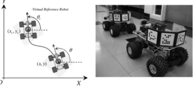
Consider the planar motion of mobile robots un-der the nonholonomic constraint of pure rolling and non-slipping, the kinematic model is given as follows(see Figure 1)
˙x ˙ y ˙ θ =
cosθ 0
sinθ 0
0 1
v
ω
, (1)
where (x,y) ∈ R2 denotes the position of the robot in a Cartesian coordinate frame, θ ∈
(−π,π]represents the orientation of the robot with respect to the positive X axis, and v ∈ V ⊆ R and ω ∈ W ⊆ R are the control in-puts representing linear and angular velocities, respectively.
Figure 1. Nonholonomic mobile robots.
Although there is no consideration of motor dy-namics and other mechanical effects, this sim-plified model is sufficient to describe the non-holonomic mobile robots’ motion.
Since system (1) falls in the form of driftless systems ˙x ˙ y ˙ θ = cosθ sinθ 0 v+ 0 0 1
ω, (2)
and the accessibility rank condition is globally satisfied[5]
rank{g1,g2,[g1,g2]}=rank
cosθ0 sinθ
sinθ 0−cosθ
0 1 0
=3, (3)
whereg1 = [cosθ sinθ 0]T, g2 = [0 0 1]T and[g1,g2]is the Lie bracket ofg1andg2, sys-tem (1)is controllable. Note that, for nonlin-ear systems, the existence of continuous time-invariant state feedback control laws cannot be implied by controllability.
2.2. Trajectory Tracking
Let a triplet zc = [x y θ]T describe the
po-sition and the orientation of a mobile robot. The reference trajectory can be described by a virtual reference robot with a state vector
zr = [xr yr θr]T, an input vectorur = [vr ωr]T
and the kinematic model(see Figure 1)
˙
zr =
˙x r ˙ yr ˙ θr = cosθ r 0
sinθr 0
0 1
ur. (4)
Then the trajectory tracking problem can be stated[15].
Problem 1. The trajectory tracking problem,
under the assumption that the virtual reference robot is not at rest (vr =ωr =0) when t → ∞,
is to find a feedback control law u = [v ω]T, such that
lim
t→∞(zr−zc) =0,
with any initial robot posturezc(0).
By transforming the reference statezr in a
lo-cal coordinate system attached to the tracking robot, an error statezecan be defined as follows
[22]
ze :=
x e ye θe =
cosθ sinθ 0
−sinθ cosθ 0
0 0 1
(zr−zc).
(5)
Taking the derivative of (5) and rearranging with(1),(4), the error model becomes
˙
xe = ωye−v+vrcosθe,
˙
ye = −ωxe+vrsinθe,
˙
θe = ωr−ω. (6)
Let us defineue,
ue:=
u1 u2 =
−v+vrcosθe
ωr−ω
, (7)
then the error model(6)becomes
˙
ze =
0 ω 0
−ω 0 0 0 0 0
ze+
0
vrsinθe
0 + 1 0 0 0 0 1
ue.
By linearizing system(8)about the the equilib-rium point(ze =0,ue=0), we obtain
˙
ze =
0 ω
r 0
−ωr 0 vr
0 0 0
ze+
1 0
0 0 0 1
ue. (9)
The controllability of system(9)can be easily checked. However, when the virtual reference robot stops (vr = ωr = 0), the controllable
property is lost.
2.3. Point Stabilization
For the point stabilization problem, one can use the following definition.
Problem 2. Given an arbitrary constant
refer-ence position and orientationzd= [xd yd θd]T,
the point stabilization problem is tofind a feed-back control lawu= [v ω]T, such that
lim
t→∞(zd−zc) =0,
with any initial robot posturezc(0).
Without loss of generality, we usezd = [0 0 0]T.
Then the problem becomes finding a feedback control law which drives system (1) back to the origin. It is a well-known fact that a smooth time-invariant feedback control law does not ex-ist for the point stabilization problem[7]. How-ever, with the analysis in Section 2.1, the system
(1)is still controllable.
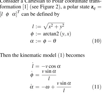
Figure 2.Coordinate transformation.
Consider a Cartesian to Polar coordinate trans-formation[1] (see Figure 2), a polar statezq =
[l φ α]T can be defined by
l := x2+y2
φ := arctan2(y,x)
α := φ −θ (10)
Then the kinematic model(1)becomes ˙
l = −vcosα ˙
φ = vsinl α
˙
α = −ω + vsinl α (11)
Note, whenl = 0, which means that the robot reaches the origin, the new kinematic model is not defined.
3. First-state Contractive MPC
Without considering disturbances and model uncertainties, systems like(6)and(11)can be generally expressed by the following nonlinear set of differential equations
˙z(t) =h(z(t),u(t)), z(0) =z0, (12)
with a state vectorz(t)∈Rmand an input vector
u(t)∈Rn,m,n∈N. Functionh:Rm×Rn→
Rmis assumed to be continuous.
Since the control system is usually implemented on a computer in discrete time,(12)can be con-verted into
z(k+1) =f(z(k),u(k)), z(0) =z0, (13)
with a state vector z(k) ∈ Z and an input vector u(k) ∈ U, k ∈ Z∗. Z ⊂ Rm is the state constraint which contains the origin in its interior. U ⊂ Rn is the input constraint
which is a compact subset of Rn containing the origin in its interior. Usually, we have U = {u ∈ Rn : u
min ≤ u ≤ umax}. umin andumax are known constants inRn. Function
f:Rm×Rn→Rmis assumed to be continuous. The control goal is to find a control sequence
equilibrium(z(k) = 0 and u(k) = 0). To ob-tain the current control u(k) at time tk, where
k is a non-negative integer (k ∈ Z∗), a finite-horizon optimal control problem
min
u JH(z,k,u),
subject to: z(k+1) =f(z(k),u(k)), z(k)∈ Z,
u(k)∈ U, (14)
must be solved online for an MPC algorithm. The performance indexJH(z,k,u)is defined as
JH(z,k,u):= H
i=1
L(z(k+i;k),u(k+i−1;k)),
(15)
whereH ∈Nis the horizon length(for simplic-ity, in this paper the prediction horizon equals the control horizon). The incremental cost is defined by
L(z,u):=z2
Q+u2R, (16)
where zQ and uR denote the weighted
2-norm, which are defined asz2
Q :=zTQzand
u2
R := uTRu. Q and R are positive definite
symmetric matrices of appropriate dimensions. Since a finite horizon is used, the controller found in (14) is not guaranteed to be stable. Many researchers have contributed to the sta-bility of nonlinear MPC with some important methods. In [26], authors propose that by adding aterminal state equality constraintz(k+ H) =0 to the optimal control problem, the sta-bility can be guaranteed. However, strong as-sumptions on the optimal control problem are required and the computational load is huge in a nonlinear case. In order to overcome those dif-ficulties, aterminal state inequality constraint
z(k+H) ∈ Ω can take the place of terminal state equality constraint[29]. Ω, a subset ofRm
containing the origin in its interior is called ter-minal region. Aterminal controlleris switched in if the state vector is inside theterminal region. This method is denoted asdual-modeMPC. A similar approach, quasi-infinite MPC, is pro-posed in[9]. In addition to theterminal inequal-ity constraint, a terminal penaltyg(z(k+H))is added to the performance index to assure stabil-ity of the system. Aterminal controller is still required, but it is never applied to the system
in the quasi-infinite MPC scheme. Although the computational load can be reduced, the dif-ficulty of dual-mode MPC and quasi-infinite MPC algorithms lies in calculating the termi-nal region (upper bounded by theregion of
at-traction of the terminal controller). An MPC
scheme withoutterminal regionrequirements is proposed by authors in [14]. A terminal con-tractive constraint g(z(k + H)) ≤ ρg(z(k)), where ρ ∈ (0, 1) is called contractive
pa-rameter, takes the place of terminal
inequal-ity constraint. Global exponential stabilinequal-ity of the closed-loop system can be guaranteed. The reader is referred to[4] for a formal definition and further details of contractive and invariant sets. Most recently a robust model predictive control algorithm blended with a reactive safety mode has been introduced in [8] for uncertain nonlinear systems. See[27]for a more detailed discussion on stability of MPC.
To achieve stability, the core idea behind the methods mentioned above is to add terminal state penalties in the performance index and impose constraints on the terminal state at the end of the prediction horizon. Therefore, those methods can be denoted as terminal-state
con-strained MPC (TSC-MPC). However, in the
implementation of most MPC schemes, only the first control of the control sequence yield by optimization is applied to the plant at each sampling instant. All the other controls are dis-carded. Only the first state at the beginning of the prediction horizon is directly affected by this implementation.
Motivated by this observation and the contrac-tiveMPC scheme developed in[14], in this pa-per we obtain the current controlu(k)at timetk
by solving the following finite-horizon optimal control problem online
min
u JH(z,k,u),
subject to: z(k+1) =f(z(k),u(k)), z(k)∈ Z,
u(k)∈ U,
z(k+1)Pˆ ≤ρz(k)Pˆ, (17) where JH(z,k,u) is defined in (15) and (16).
ˆ
P is a positive definite symmetric matrix and
ρ∈(0, 1).
This means that the first state at the begin-ning of the prediction horizon,z(k+1)is con-tracted in norm with respect to the current state,
z(k). Therefore, the proposed MPC algorithm can be denoted as first-state contractive MPC
(FSC-MPC). The user adjustable parameterρis calledcontractive parameter, which addresses the contraction rate.
The FSC-MPC controller can be implemented as follows.
FSC-MPC Algorithm
Data: prediction horizon H ∈ N; sampling time δT ∈ R+; weights Q, R, ˆP > 0;
con-straintsumin,umax ∈Rm; contractive parameter
ρ∈(0, 1);k∈Z∗.
Step 0: setk = 0; set initial control prediction ˆ
u(i;k) =0,i∈[1, . . . ,H−1].
Step 1: measure the statesz(k)at timetk; with
control prediction ˆu(i;k), solve the optimal con-trol problem(17)and obtain a control sequence
u∗(i;k).
Step 2: apply the first control u∗(1;k) in the control sequenceu∗(i;k)to system(13)for the time interval[tk, tk+1], wheretk+1=tk+δT.
Step 3: update the control prediction as follows
ˆ
u(i;k) =
u∗(i+1;k) i∈[1, . . . ,H−2]
u∗(i;k) i=H−1 ;
setk=k+1; go back toStep 1.
Note, in Step 1, an assumption is that for all k ∈ Z∗, a feasible solution of the optimal con-trol problem(17), satisfying all the constraints, always exists. However, globally optimal solu-tion is not strictly required here. Locally op-timal or less opop-timal solutions are acceptable. This approach might compromise the perfor-mance, but the stability property of the algo-rithm will not be affected.
4. Stability Results
In this section, the stability of the FSC-MPC algorithm will be proven. Before we give the main result, let’s make the following assump-tions[14].
Assumption 3. There exists a constant β ∈
(0, ∞) such that for all z(k) ∈ Bβ := {z ∈
Z|zPˆ ≤ β}, a contractive parameter ρ ∈
(0, 1) can be found so that at time tk, a
feasi-ble solution of the optimal control profeasi-blem (17), satisfying all the constraints, always exists for all k ∈Z∗.
Note that Assumption 3 means that there is a nonempty convex and compact set of initial conditions such that the optimal control prob-lem is feasible. It is restrictive but still ac-ceptable. As pointed out by authors in [6], if
[(∂h/∂z)(∂h/∂u)] ∈ Ω¯, ∀z, u, where ¯Ω ⊆
Rm×(m+n), the nonlinear system can be replaced by a time-varying linear system in linear
dif-ferential inclusions form by using global
lin-earization techniques. Then sufficient
condi-tions for Assumption 3 can be found by using a single quadratic Lyapunov function(details can be found in[3], where sufficient conditions for exponential stability and an inducedL2−norm performance objective are given).
Assumption 4. For all t ∈[tk, tk+1], k∈ Z∗, there exists a constant κ ∈ (0, ∞), such that the transient state, z(t), satisfies z(t)Pˆ ≤
κz(k)Pˆ.
Note that Assumption 4 means that systems with finite escape time are not under consideration.
Theorem 5. Suppose that the optimal control
problem is feasible at time t0and Assumptions
3 and 4 are satisfied. The FSC-MPC algorithm
described in Section 3 for system (12), (13) is exponentially stable in the sense that the state trajectory of the closed-loop system satisfies the following inequality
z(t)Pˆ ≤κz(0)Pˆe−
(1−ρ)
δT (t−t0), (18)
whereδT is the sampling time.
Proof: Since the optimal control problem is fea-sible at timet0, from Assumption 3, the optimal control problem is feasible at time tk, k ∈ Z∗.
Therefore, we have
z(k)Pˆ≤ρz(k−1)Pˆ≤ · · · ≤ρkz(0)Pˆ.
Now with Assumption 4 and(19),z(t)satisfies the following inequality
z(t)Pˆ ≤κρkz(0)Pˆ, (20) wheret∈[tk, tk+1], for allk∈Z∗.
Since ρ ∈ (0, 1), we have e(ρ−1) −ρ ≥ 0, which meanse(ρ−1)k ≥ρk ≥ 0, for allk∈Z∗.
Inequality(20)can be rewritten as follows
z(t)Pˆ ≤κz(0)Pˆe−(1−ρ)k. (21)
Since k = (tk − t0)/δT and (t − t0)/δT ≤
(tk−t0)/δT =k, for allt∈[t0, tk], we have
e−(1−ρ)k ≤e−(1δ−Tρ)(t−t0) (22)
Therefore, from inequalities(21)and(22), we conclude
z(t)Pˆ ≤κz(0)Pˆe−
(1−ρ)
δT (t−t0).
According to [23], the closed-loop system is exponentially stable, so is the FSC-MPC algo-rithm.
5. Simulation Results
The effectiveness of the FSC-MPC algorithm presented in Section 3 is investigated by numer-ical simulations. In the figures, each robot is depicted by an arrow within a circle(dotted cir-cle for virtual reference robots). The orientation of the robot is shown by the orientation of the arrow.
The units used in the simulations are: for po-sition, meter(m), for orientation, radian(rad), for linear velocity, meter/second(m/s), and for angular velocity, radian/second(rad/s).
5.1. Trajectory Tracking
In this section, the simulation results of our FSC-MPC controller, Kanayama’s controller pro-posed in[22]and Samson’s controller proposed in [15] are compared. Specifically, the con-trollers proposed in[22]and[15]are
v
ω
=
vrcosθe+Kxxe
ωr+vr(Kyye+Kθsinθe)
, (23)
and
v
ω
=
v
rcosθe+K1xe
ωr +K2vrsinθeθe +K3θe
, (24)
respectively.
The reference trajectory starts from posture
zr(0) = [0 0 0]T with constant control inputs
[vr ωr]T = [1 0]T. In addition, we assume
that two perturbations occur at times 10 s and 20 s which changes the orientation of the vir-tual reference robot from 0 rad toπ/2 rad and fromπ/2 rad back to 0 rad, respectively. Total simulation time is 30 s.
The initial condition of tracking robot iszc(0) =
[0 3 0]T. Controller parameters are selected as follows. For Kanayama’s controller, Kx = 1,
Ky = 4 and Kθ = 4. For Samson’s controller,
K1 = 1, K2 = 4 and K3 = 4. Sampling time for these two controllers is δT = 0.1 s. For
FSC-MPC controller,H =6,ρ=0.95,
Q=
5 0 0
0 5 0 0 0 1
, R=I2×2, Pˆ =I3×3, (25)
where Ir×r denotes the r ×r identity matrix.
Sampling time is δT = 0.5 s. Control input
constraints are
−4(m/s)≤v≤4(m/s), −0.8(rad/s)≤ω ≤0.8(rad/s).
The system responses of the three controllers are shown in Figure 3. The FSC-MPC con-troller successfully stabilizes the tracking robot to the reference trajectory.
Figure 3.Tracking trajectories of three controllers. Dashed: Reference. Solid: FSC-MPC. Dotted: Samson.
Initial Posture Aicardi’s Controller FSC-MPC Controller
[1 0 π/2]T 1772.7122 10.4999
[−0.5 0.867 π/2]T 586.2641 6.1507
[−0.5 −0.867 π/2]T 69.7075 3.7015
Table 1.The integral of norm squared actual control inputs for stabilization.
5.2. Point Stabilization
In this section, the simulation results of our FSC-MPC controller and Aicardi’s controller proposed in[1]are compared. Specifically, the controller proposed in[1]is
v
ω
=
K1ecosα
k2α +K1cosααsinα(α +K3φ)
. (26)
Three initial robot postures are used in the sim-ulation. They are
zc(0) =
1 0
π/2
,
−0.5
0.867
π/2
,
−0.5 −0.867
π/2
.
The final posture is zd = [0 0 0]T.
Con-troller parameters are selected as follows. For Aicardi’s controller, K1=3, K2=6 and K3=1. For FSC-MPC controller, controller parameters, sampling time and control input constraints are the same as those in Subsection 5.1.
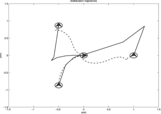
The trajectories generated by Aicardi’s con-troller and our FSC-MPC concon-troller from differ-ent initial postures are shown in Figure 4. The
Figure 4.Stabilizing trajectories of two controllers. Solid: FSC-MPC. Dashed: Aicardi.
FSC-MPC controller successfully stabilizes the robot at the desired final posture.
Specifically, we use the integral of norm squared actual control inputs (k1u2δ
T) as a metric
to evaluate the control energy. The control en-ergy expended by each controller from differ-ent initial postures are shown in Table 1. The FSC-MPC requires much less control energy in comparison with the Aicardi’s controller.
5.3. Simultaneous Tracking and Stabilization
In this section, numerical simulations illustrate that our FSC-MPC controller has the ability of simultaneous tracking and stabilization. Usu-ally, simultaneous tracking and stabilization is not considered under a single controller ap-proach. Most of the existing controllers for tra-jectory tracking of nonholonomic mobile robots will fail when the virtual reference robot stops or moves backward. However, in realistic sce-narios, we do need to handle those situations. In simulation, the virtual reference robot starts moving backward from posture zr(0)=[0 0
π/2]T with constant control inputs[v
r ωr]T =
[−1 0.1]T. Then, it stops at time t = 5 s. The initial condition of the tracking robot is
zc(0) = [10 10π/2]T. We compare our
FSC-MPC controller with Samson’s controller(24). Controller parameters, sampling time, simula-tion time and control input constraints are the same as those in Subsection 5.1.
Figure 5.Trajectories of simultaneous tracking and stabilization. Dashed: Reference. Solid: FSC-MPC.
Dash-Dot: Samson.
6. FSC-MPC Formation Control
In this section, we consider using the FSC-MPC algorithm proposed in Section 3 to solve the problem of controlling a team of mobile robots with nonholonomic constraints to leader-following formations. Since the FSC-MPC al-gorithm has simultaneous tracking and point stabilization capability, we expect that it can keep the formation in real-world scenarios. The effectiveness of the method is investigated by numerical simulations.
6.1. Formation Error
Let a tripletpi = [xi yi θi]T describe the
posi-tion and the orientaposi-tion of theith mobile robot. A leader-following formation configurationFijd between robotiandjcan be defined by the de-sired relative distancesΔxdij and Δydij in a local coordinate frame attached to the leader roboti, whereFdij=Δxdij ΔydijT.
However, to directly use the results in Section 3, we need to convert the formation control prob-lem to a trajectory tracking probprob-lem. Let us define a reference robot, whose position and orientation are as follows
xr := xi+lcos(η),
yr := yi+lsin(η), (27)
θr := θi,
where
l = Δxd ij
2
+Δyd ij
2
,
η = arctan2(Δydij,Δxdij) +θi. (28)
Now we can define the formation error for the jthrobot, which is a tracking error defined by
xej :=
x
r−xj
yr−yj
θr−θj
. (29)
Figure 6 shows this conversion.
Figure 6.Convert formation control to trajectory tracking.
Let us define the optimal control problem for robotj, we have
min
u J
H
j (xej,k,uj),
subject to: xej(k+1) =f(xej(k),uj(k)),
xej(k)∈ X,
uj(k)∈ U,
xej(k+1)Pˆ ≤ρxej(k)Pˆ, (30)
whereJjH(xej,k,uj)is defined as
JjH(xej,k,uj):= H
i=1
L(xej(k+i;k),uj(k+i−1;k)),
(31)
where
The FSC-MPC formation controller can be im-plemented as follows.
Data: prediction horizon H ∈ N; sampling time δT ∈ R+; weights Q, R, ˆP > 0;
con-straintsumin,umax ∈Rm; contractive parameter
ρ∈(0, 1);k∈Z∗; desired formationFd ij.
Step 0: setk = 0; set initial control prediction ˆ
ui(s;k) =uˆj(s;k) =0,s∈[1, . . . ,H−1].
Step 1: receive leader statespi(k), control
pre-diction ˆui(s;k) and measure the states pj(k)
at time tk; with control prediction ˆui(s;k) and
ˆ
uj(s;k), desired formationFdijand relations(27),
(28)and (29), solve the optimal control prob-lem(30)and obtain a control sequenceu∗j(s;k).
Step 2: apply the first control u∗j(1;k) in the control sequenceu∗
j(s;k)to robotjfor the time
interval[tk, tk+1], wheretk+1 =tk+δT.
Step 3: update the control prediction as follows
ˆ
uj(s;k) =
u∗j(s+1;k) s∈[1, . . . ,H−2]
u∗j(s;k) s=H−1 ;
setk=k+1; go back toStep 1.
6.2. Simulation Results
The effectiveness of the FSC-MPC formation control algorithm is investigated by numerical simulations.
6.2.1. Reconfiguration
In this simulation, we consider a formation re-configuration scenario. We assume that the leader robot has the ability to sense the environ-ment and communicate with each robot in the team. During the navigation, the leader detects a wall and sends commands to follower robots to change the formation to a line such that they can pass a small gate. After all the robots pass the gate, the leader sends commands to resume the previous formation.
The leader robot starts moving from posture
p1(0) = [0 0 0]T with constant control in-puts [v1 ω1]T = [1 0]T. Robot 2 and 3 start from p2(0) = [−8 −1 π/4]T and p3(0) =
[−15 −3 −π/4]T. The desired formation is F12d = [−5 2]TandFd23 = [−5 −4]T. At time t = 15 s, the leader detects the wall and sends commands to team robots to change to a new formationFd12 = [−5 0]T andF23d = [−5 0]T, which is a line formations. At timet = 30 s, as all the robots have passed the gate, the leader sends commands again and changes the forma-tion back to the original one F12d = [−5 2]T
andF23d = [−5 −4]T.
The control parameters for the FSC-MPC for-mation controller are H = 3, ρ = 0.999. Q, Rand ˆPare the same as in(25). Control input constraints are
−4(m/s)≤v≤4(m/s),
−0.5(rad/s)≤ω ≤0.5(rad/s).
Sampling time isδT =0.5 s and the total
sim-ulation time is 50 s.
Figure 7 depicts the trajectories of the robot team. We can see that the triangle formation is kept before and after the change to a line for-mation and the line forfor-mation is achieved when the team passes the gate.
Figures 8 and 9 show the control inputs and the relative position of Robot 2. In Figure 9, we can see that the actual relative position of Robot 2 converges to the desired formation Fd
12 = [−5 2]T beforet =15 s and aftert=30 s and the desired formationFd
12 = [−5 0]T dur-ing time[15 30]. In Figure 8 we can see that, when the formation is achieved, the control in-puts converge to[1 0]T, which are the velocities
of the leader robot.
Figures 10 and 11 show the control inputs and the relative position of Robot 3. In Figure 11, we can see that the actual relative posi-tion of Robot 3 converges to the desired for-mation F23d = [−5 −4]T before t = 15 s and after t = 30 s and the desired formation F23d = [−5 0]T during time[15 30]. Figure 10 shows that, when the formation is achieved, the control inputs converge to[1 0]T, which are the
Figure 7.Reconfiguration during navigation.
Figure 8.Control inputs of Robot 2.
Figure 9.Relative position of Robot 2.
6.2.2. Obstacle Avoidance
In this simulation, we consider an obstacle avoid-ance scenario. We assume that the leader robot has the ability to sense the environment. During navigation, the leader robot detects an obstacle. It stops and then moves backward, stops and
Figure 10.Control inputs of Robot 3.
Figure 11.Relative position of Robot 3.
moves forward for several times to make sure the whole team will not collide with the obsta-cle. Finally, the team moves forward again in formation.
The leader robot starts moving from posture
p1(0) = [0 0 0]T. The leader robot’s veloc-ity inputs are
v1
ω1
=
⎧ ⎪ ⎪ ⎪ ⎪ ⎪ ⎪ ⎪ ⎪ ⎪ ⎪ ⎪ ⎪ ⎪ ⎪ ⎪ ⎨ ⎪ ⎪ ⎪ ⎪ ⎪ ⎪ ⎪ ⎪ ⎪ ⎪ ⎪ ⎪ ⎪ ⎪ ⎪ ⎩
[1 0]T t= [0 15], [0 0]T t= [15.5 20], [−1 −0.15]T t= [20.5 25], [0 0]T t= [25.5 30], [1 0.15]T t= [30.5 35], [0 0]T t= [35.5 39.5], [1 0]T t=40,
[−1 −0.15]T t= [40.5 45], [0 0]T t= [45.5 50], [1 0]T t= [50 60],
de-sired formation is Fd
12 = [−5 2]T and Fd23 =
[−5 −4]T.
Control parameters for the FSC-MPC formation controller are,H = 4,ρ = 0.999. MatricesQ, R, ˆP are chosen as (25). Control input con-straints are
−4(m/s)≤v≤4(m/s),
−0.5(rad/s)≤ω ≤0.5(rad/s).
Sampling time isδT = 0.5 s and the total
sim-ulation time is 60 s.
Figure 12 shows the trajectories of the robot team. We can see that the triangle formation is kept. Figure 13 depicts the control inputs of Robot 2. In addition, Figures 14 and 15 present the control inputs and the relative position of Robot 3. In Figure 15, we can see that the actual relative position of Robot 3 converges to
Figure 12.Obstacle avoidance during navigation - three robots.
Figure 13. Control inputs of Robot 2.
Figure 14.Control inputs of Robot 3.
Figure 15.Relative position of Robot 3.
the desired formationFd
23 = [−5 −4]T. How-ever, by comparing Figures 13 and 14, we can see that Robot 3 requires more control authority than Robot 2.
7. Conclusions
For all simulations, an initial feasible solution is required for the proposed FSC-MPC controller. Like most of the MPC schemes, a trial-and-error approach is used. The choice of the contractive parameter is critical for the initial feasible so-lution. A value close to 1 is preferred. How-ever, a small value will give faster convergence rate when the system approaches the equilib-rium point. As part of our future work, we are investigating adaptive or time-varying schemes of the contractive parameter, and experimental verifications of the FSC-MPC on our experi-mental testbed[12].
Acknowledgment
This work is supported in part by NSF grants CAREER #0811347 and CNS #0709329, and the U.S. Army Research Office grant DAAD19-03-1-0142 (through the University of Okla-homa). We would like to thank the anony-mous reviewers for their insightful comments and suggestions.
References
[1] M. AICARDI, G. CASALINO, A. BICCHI, AND A. BALESTRINO, Closed loop steering of unicycle-like vehicles via Lyapunov techniques.IEEE Robot. Automat. Mag., pages 27–35, March 1995.
[2] A. ASTOLFI. Exponential stabilization of a wheeeled mobile robot via discontinuous control. J. Dynam. Syst. Meas., 121:121–126, 1999.
[3] G. BECKER, A. PACKARD, D. PHILBRICK, AND G. BALAS. Control of parametrically-dependent linear systems: A single quadratic lyapunov ap-proach. In Proceedings of the American Control Conference, volume 3, pages 2795–2799, San Fran-cisco, CA, June 1993.
[4] F. BLANCHINI. Set invariance in control. Automat-ica, 35:1747–1767, 1999. Survey paper.
[5] A. M. BLOCH.Nonholonomic Mechanics and Con-trol. Springer, New York, NY, 2003.
[6] S. BOYD, L. E. GHAOUI, E. FERON,ANDV. BALAKR-ISHNAN. Linear Matrix Inequalities in System and Control Theory, volume 15 of Studies in Applied Mathematics. SIAM, Philadelphia, 1994.
[7] R. W. BROCKETT. Asymptotic stability and feed-back stabilization. In R. W. Brockett, R. S. Millman, and H. J. Sussmann, editors, Diferential Geomet-ric Control Theory, pages 181–191, Birkh¨auser, Boston, MA, 1983.
[8] J. CARSON, B. ACIKMESE, R. MURRAY, AND D. MACMYNOWSKI. A robust model predictive control algorithm with a reactive safety mode. In International Federation of Automatic Control (IFAC) World Congress, Seoul, Korea, July 6-11 2008. To appear.
[9] H. CHEN ANDF. ALLGOWER. A quasi-infinite hori-zon nonlinear model predictive scheme with guar-anteed stability. Automatica, 14(10):1205–1217, 1998.
[10] D. CHWA. Sliding-mode tracking control of non-holonomic wheeled mobile robots in polar co-ordinates. IEEE Trans. Contr. Syst. Technol., 12(4):637–644, 2004.
[11] R. COLBAUGH, E. BARANY,ANDK. GLASS. Adap-tive control of nonholonomic robotic systems. J. Robotic Systems, 15(7):365–393, 1998.
[12] D. CRUZ, J. MCCLINTOCK, B. PERTEET, O. ORQUEDA, Y. CAO,ANDR. FIERRO. Decentralized cooperative control: A multivehicle platform for research in networked embedded systems. IEEE Control Syst. Mag., 27(3):58–78, June 2007.
[13] A. K. DAS, R. FIERRO, V. KUMAR, J. P. OSTROWSKI, J. SPLETZER,ANDC. J. TAYLOR. A vision-based for-mation control framework. IEEE Transactions on Robotics and Automation, 18(5):813–825, October 2002.
[14] S. L.DEOLIVEIRAKOTHARE ANDM. MORARI. Con-tractive model predictive control for constrained nonlinear systems. IEEE Trans. Automat. Contr., 45(6):1053–1071, 2000.
[15] C. CANUDAS DE WIT, H. KHENNOUF, C. SAMSON, ANDO. J. SORDALEN. Nonlinear control design for mobile robots. In Y. F. Zheng, editor,Recent Trends in Mobile Robot, chapter 5, pages 121–156. World Scientific, 1993.
[16] W. E. DIXON, D. M. DAWSON, E. ZERGEROGLU,AND A. BEHAL. Nonlinear control of wheeled mobile robots. Springer, London, UK, 2001.
[17] R. FIERRO ANDF. L. LEWIS. Control of a nonholo-nomic mobile robot: Backstepping kinematics into dynamics. InProceedings of the IEEE Conference on Decision and Control, pages 3805–3810, New Orleans, LA, December 1995.
[18] R. FIERRO ANDF. L. LEWIS. Robust practical point stabilization of a nonholonomic mobile robot using neural networks.Journal of Intelligent and Robotic Systems,(20):295–317, 1997.
[19] D. GU ANDH. HU. A stabilizing receding horizon regulator for nonholonomic mobile robots. IEEE Trans. Robot. Automat., 21(5):1022–1028, October 2005.
[21] G. INDIVERI. Kinematic time-invariant control of a 2D nonholonomic vehicle. In Proceedings of the IEEE Conference on Decision and Control, pages 2112–2117, Phoenix, AZ, December 1999.
[22] Y. KANAYAMA, Y. KIMURA, F. MIYAZAKI, AND T. NOGUCHI. A stable tracking control method for an autonomous mobile robot. InIEEE Int. Conf. on Robotics and Automation, pages 384–389, 1990.
[23] H. K. KHALIL. Nonlinear Systems. Prentice Hall, third edition, 2002.
[24] H. KHENNOUF AND C. C. DE WIT. On the con-struction of stabilizing discontinuous controllers for nonholonomic systems. InIFAC Nonlinear Control Syst. Design Symp., pages 747–752, Tahoe City, CA, 1995.
[25] B. KIM ANDP. TSIOTRAS. Controllers for unicycle-type wheeled robots: Theoretical results and exper-imental validation. IEEE Trans. Robot. Automat., 18(3):294–307, 2002.
[26] D. Q. MAYNE ANDH. MICHALSKA. Receding hori-zon control of nonlinear systems. IEEE Trans. Automat. Contr., 35(7):814–824, 1990.
[27] D. Q. MAYNE, J. B. RAWINGS, C. V. RAO, AND P. O. M. SCOKAERT. Constrained model predic-tive control: Stability and optimality. Automatica, 36(6):789–814, June 2000.
[28] R. T. M’CLOSKEY ANDR. M. MURRAY. Exponential stabilization of driftless nonlinear control systems using homogeneous feedback. IEEE Trans. Au-tomat. Contr., 42(5):614–628, May 1997.
[29] H. MICHALSKA ANDD. Q. MAYNE. Robust receding horizon control of constrained nonlinear systems. IEEE Trans. Automat. Contr., 38(11):1623–1633, November 1993.
[30] P. MORIN ANDC. SAMSON. Practical stabilization of a class of nonlinear rsystems: Application to chain systems and mobile robots. In Proceedings of the IEEE Conference on Decision and Control, pages 2144–2150, Sydney, Australia, 2000.
[31] R. M. MURRAY. Recent research in cooperative control of multivehicle systems. ASME Journal of Dynamic Systems, Measurement, and Control, 129(5):571–583, September 2007.
[32] R. M. MURRAY, Z. LI,ANDS. S. SASTRY.A Mathe-matical Introduction to Robotic Manipulation. CRC Press, 1993.
[33] G. ORIOLO, A. DE LUCA, AND M. VENDITTELLI. WMR control via dynamic feedback linearization: Design, implementaion, and experimental valida-tion. IEEE Trans. Contr. Syst. Technol., 10(6):835– 852, 2002.
[34] J. B. POMET. Explicit design of time-varying sta-bilizing control laws for a class of controllable systems without drift. Systems and Control Letters, 18:147–158, 1992.
[35] C. SAMSON. Control of chained systems. Appli-cation to path following and time-varying point-stabilizaiton of mobile robots. IEEE Trans. Au-tomat. Contr., 40:64–77, Jan. 1995.
[36] C. SAMSON AND K. AIT-ABDERRAHIM. Feedback control of a nonholonomic wheeled cart in Carte-sian space. In IEEE Int. Conf. on Robotics and Automation, pages 1136–1141, Sacramento, CA, 1991.
[37] M. J. VACHON, R. J. RAY, K. R. WALSH,ANDK. EN-NIX. F/a-18 performance benefits measured during the autonomous formation flight project. Technical Report NASA/TM-2003-210734, NASA Dryden Flight Research Center, Edwards, California., 2003. [38] G. C. WALSH, D. TILBURY, S. SASTRY, R. MURRAY, AND J. P. LAUMOND. Stabilization of trajectory for systems with nonholonomic constraints. IEEE Trans. Automat. Contr., 39:216–222, Jan. 1994. [39] J. WAN, C. G. QUINTERO, N. LUO,ANDJ. VEHI.
Pre-dictive motion control of a MiRoSoT mobile robot. InProceedings of World Automation Congress, vol-ume 15, pages 325–330, 2004.
[40] D. WANG ANDG. XU. Full-state tracking and in-ternal dynamics of nonholonomic wheeled mo-bile robots. IEEE/ASME Trans. Mechatronics, 8(2):203–214, 2003.
Received:December, 2007 Revised:May, 2008 Accepted:June, 2008
Contact addresses: Feng Xie School of Electrical and Computer Engineering Oklahoma State University Stillwater, USA e-mail:[email protected]
Rafael Fierro The MARHES Lab, Department of Electrical & Computer Engineering MSC01 1100 1 University of New Mexico Albuquerque, NM 87131-0001, USA e-mail:[email protected]
FENGXIEreceived a B.Sc. degree in testing technology and instru-mentation and a M.Sc. degree in control science and engineering from Zhejiang University, China in 1997 and 2000, respectively. He received a second M.S. degree in chemical engineering and a Ph.D. degree in electrical engineering from Oklahoma State University in 2004 and 2007, respectively. His research interests include cooperative control of mobile robots, model predictive control and nonlinear control theory.