Grinias_unc_0153D_14877.pdf

(1)

CHARACTERIZATION AND CONTROL OF BAND BROADENING IN ULTRA-HIGH PRESSURE LIQUID CHROMATOGRAPHY COLUMNS

James P. Grinias

A dissertation submitted to the faculty of the University of North Carolina at Chapel Hill in partial fulfillment of the requirements for the degree of Doctor of Philosophy in the

Department of Chemistry.

Chapel Hill 2014

(2)

(3)

ABSTRACT

James P. Grinias: Characterization and Control of Band Broadening in Ultra-High Pressure Liquid Chromatography Columns

(Under the direction of James W. Jorgenson)

Improving column performance remains paramount to advancing liquid chromatography (LC) technology. To that end, a series of experiments was designed to both measure and reduce band broadening in LC columns. The main broadening mechanisms (multiple flow path

dispersion, longitudinal molecular diffusion, and resistance to mass transfer) were investigated. Dispersion due to multiple flow paths within a packed bed were studied with a series of columns prepared using different packing conditions. Packed column microstructure was analyzed by confocal laser scanning microscopy (CLSM) to determine bed morphology. Column efficiency was correlated to the bed morphology and the radial particle size distribution. Research on longitudinal molecular diffusion focused on the validity of different stationary phase diffusion models. Evidence was found supporting the recently proposed surface-restricted model of surface diffusion. This result has implications affecting both gradient separations and the

(4)

(5)

ACKNOWLEDGEMENTS

First, I must thank my research advisor Professor Jim Jorgenson for his guidance and advice over the past five years. His enthusiasm for chromatography was contagious and helped motivate me to grow as a scholar and a scientist. Many of my colleagues from the Jorgenson lab also deserve my deepest gratitude. Ed Franklin and Laura Blue took me under their wing when I first started and have been great mentors ever since; the capillary columns presented in Chapter 2 were a combined, group effort. Justin Godinho has been a dependable co-worker and friend throughout my final two years of graduate school; his contributions to column preparation in Chapter 4 were vital. Other colleagues who have helped me are James Treadway, Dan Lunn, Stephanie Moore, Jordan Stobaugh, and Brian Matthew by providing advice, assistance, know-how, and camaraderie over the past few years. My two undergraduate mentees (Dayley Wilson and Alison Ivey) were very helpful in the data collection for Chapter 5. Finally, I cannot begin to express how important Kaitlin Fague was to my time at Carolina both personally and

professionally. Thank you Kaitie for all you have done… our journey is just beginning!

(6)

grateful for the particles, data, and know-how that they have provided over the past year. We would have never been able to connect with the Skrabalak lab if not for Professor Milos Novotny (and his former student Dr. Benjamin Mann); his vast knowledge of chromatography and upbeat attitude have made this a rather enjoyable collaboration. The importance of Waters Corporation to the completion of this dissertation (especially Chapters 3, 5, and 6) cannot be overstated. Dr. Geoff Gerhardt, Dr. Kevin Wyndham, Dr. Keith Fadgen, Bob Collamati, Dr. Greg Roman, and many others have all provided expertise, columns, equipment, and materials whenever needed and I have enjoyed getting to know all of them over the past five years. Special thanks must go to Waters scientists Dr. Martin Gilar and Dr. Bernard Bunner for their hard work and dedication while collaborating on Chapter 3 as well as providing me with a unique perspective on

chromatography from the industry point-of-view.

I would be remiss to not mention the many people who have helped me get to this point. Countless friends and family members must be thanked, especially my parents and sister whose unwavering support has allowed me to reach this point. My “adopted” family of St. Barbara’s Greek Orthodox Church helped me feel at home at North Carolina; they have ensured that I don’t

(7)

TABLE OF CONTENTS

LIST OF TABLES ... xii

LIST OF FIGURES ... xiii

LIST OF ABBREVIATIONS ... xxiv

LIST OF SYMBOLS ... xxvii

CHAPTER 1. Introduction to Band Broadening Theory ... 1

1.1 Overview ... 1

1.2 Band Broadening Theory ... 1

1.2.1 The Basics of Separations and Separation Terminology ... 1

1.2.2 van Deemter Theory ... 3

1.2.3 Coefficient Estimates, Reduced Parameters and Alternate Equations ... 7

1.3 Ultra-High Pressure Liquid Chromatography (UHPLC) ... 11

1.3.1 Comparison of HPLC and UHPLC... 11

1.3.2 Pressure, Flow, and Frictional Heating ... 12

1.3.3 Extra-Column Band Broadening... 14

1.4 Dissertation Scope ... 14

1.5 FIGURES ... 16

1.6 REFERENCES ... 19

CHAPTER 2. Correlation of Separation Efficiency and Bed Morphology in Packed Capillary UHPLC Columns... 21

(8)

2.1.2 Column Imaging and Reconstruction by Confocal Laser Scanning

Microscopy ... 24

2.2 Materials and Methods ... 26

2.2.1 Chemicals and Materials ... 26

2.2.2 Preparation and Analysis of 10-75 μm i.d. Capillary UHPLC Columns ... 27

2.2.3 Microscopic Imaging and Bed Reconstruction of Capillary UHPLC Columns ... 29

2.3 Results and Discussion ... 30

2.3.1 Efficiency of Capillary UHPLC Columns with Varying Aspect Ratio ... 30

2.3.2 Morphology of Capillary UHPLC Columns with Varying Aspect Ratio ... 31

2.3.3 Particle Size Segregation in Capillary UHPLC Columns ... 34

2.3.4 Slurry Concentration Effects on Efficiency and Particle Size Segregation ... 35

2.4 Conclusions ... 37

2.5 TABLES ... 40

2.6 FIGURES ... 43

CHAPTER 3. Investigation of Surface Diffusion Models and Implications for Chromatographic Band Broadening ... 68

3.1 Introduction ... 68

3.1.1 Surface Diffusion Effects in Gradient LC ... 68

3.1.2 Longitudinal Molecular Diffusion ... 69

3.1.3 Surface-Restricted Molecular Diffusion Model ... 71

3.1.4 Particle-Restricted Molecular Diffusion Model ... 74

(9)

3.2.1 Chemicals ... 75

3.2.2 Chromatographic Columns and Instrumentation ... 76

3.2.3 Variance Measurements Using Stop-Flow Techniques ... 76

3.3.1 Comparison of Surface Diffusion Models ... 78

3.3.2 Investigation of the Surface-Restricted Molecular Diffusion Model ... 79

3.3.3 Correlation Between Longitudinal Molecular Diffusion and Retention ... 80

3.5 FIGURES ... 83

CHAPTER 4. Sub-2 μm Perfusion Chromatography Particle Performance and Size Refinement by Hydrodynamic Chromatography ... 94

4.1.1 Perfusion Chromatography ... 94

4.1.2 Macroporous Silica Particle Synthesis by Ultrasonic Spray Pyrolysis ... 97

4.1.3 Sub-2 μm Macroporous Particles for Capillary UHPLC ... 98

4.2 Theory of Hydrodynamic Chromatography ... 101

4.3.1 HDC Column Preparation and Use ... 103

4.3.2 HDC Analysis and Refinement of Silica Particles ... 104

4.4.1 Separation of Nonporous Silica Size Standards by HDC ... 105

(10)

4.6 FIGURES ... 113

CHAPTER 5. Thermal Broadening Effects in Sub-2 μm Fully Porous and Superficially Porous Particle UHPLC Columns ... 135

5.1.1 Viscous Heating in UHPLC ... 135

5.1.2 Superficially Porous Particles as a Solution to Viscous Heating ... 137

5.2.1 Chemicals ... 138

5.2.2 Chromatographic Columns and Instrumentation ... 139

5.2.3 Temperature Measurement and Control Methods ... 140

5.2.4 Chromatographic Efficiency Experiments ... 141

5.3.1 Column Temperature Measurements ... 142

5.3.2 Effect of Particle Structure on Performance and Temperature ... 143

5.3.3 Effect of Column Dimensions on Performance and Temperature ... 145

5.3.4 Effect of Temperature Environment on Performance and Temperature ... 148

5.3.5 Thermal Effects on Peak Capacity of Peptides in Gradient LC ... 152

5.5 TABLES ... 157

5.6 FIGURES ... 159

(11)

6.2 Theory of Extra-Column Band Broadening ... 190

6.2.1 System Contributions to Band Broadening... 190

6.2.2 Injector Contributions ... 191

6.2.3 Exponential Decay Flow Paths ... 191

6.2.4 Connecting Tubing... 192

6.2.5 Detector Contributions ... 193

6.2.6 Calculating Peak Variance ... 194

6.3.1 Reagents and Materials ... 195

6.3.2 Subtraction Method Instrumentation and Techniques ... 195

6.3.3 Direct Measurement Instrumentation and Techniques ... 196

6.3.4 Flow Modeling Simulations ... 198

6.3.5 Extra-Column Broadening Effects on Microfluidic LC Performance ... 198

6.4.1 Broadening in Small Inner Diameter Connecting Capillaries ... 199

6.4.2 Simulations of Broadening in Injectors and Connecting Tubing... 204

6.4.3 Peak Injection Profiles ... 206

6.4.4 Efficiency Loss from ECBB in Microfluidic LC ... 207

6.6 FIGURES ... 210

(12)

LIST OF TABLES

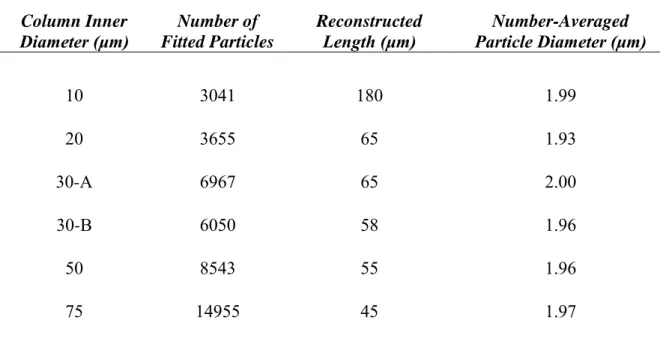
Table 2-1. Bed reconstruction parameters for six capillary LC columns packed

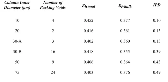
with 1.9 μm BEH particles. ... 40 Table 2-2. Morphological data for six capillary LC columns packed with 1.9 μm

BEH particles. Packing voids describe open spaces in the packed bed that

are larger than the first quartile of the overall particle size distribution. ... 41 Table 2-3. Morphological data for four capillary LC columns packed with 1.7 μm

(13)

LIST OF FIGURES

Figure 1-1. Multiple flow path broadening terms present in packed

chromatographic beds (according to the Giddings model4): transchannel (1), short-range interchannel (2), transcolumn (3), long-range interchannel

(4), transparticle (5). ... 16 Figure 1-2. Theoretical h-v plot based on Equation 1-21 with individual

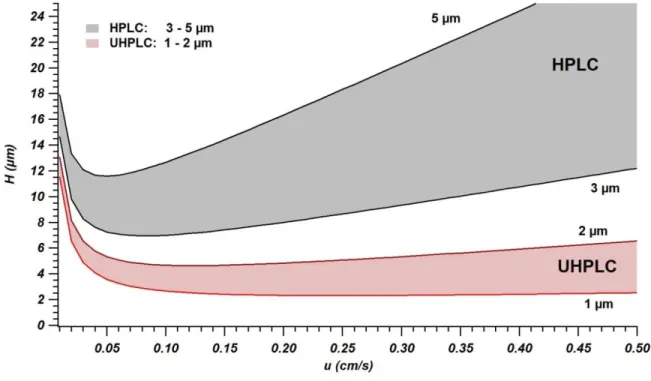
contributions from ha, hb, and hc also shown. ... 17 Figure 1-3. Comparison of relative H values for particle sizes typical of HPLC

(3-5 μm) and UHPLC (1-2 μm) based on Equation 1-17 (with Dm = 1 x 10-6

cm2/s). ... 18 Figure 2-1. Multiple flow path broadening terms present in packed

chromatographic beds (according to the Giddings model2): transchannel (1), short-range interchannel (2), transcolumn (3), long-range interchannel

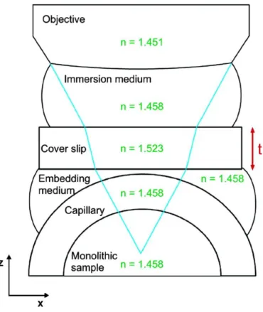
(4), transparticle (5). ... 43 Figure 2-2. Microscope scheme used to image monolithic chromatographic bed

inside a polyimide-coated fused silica capillary. A glycerol/water mixture is used as both the immersion and embedding medium, with a

DMSO/water mixture flowed through the column for refractive index matching purposes. Used with permission from Bruns, S., Müllner, T., Kollmann, M., Schachtner, J., Höltzel, A., Tallarek, U. Analytical Chemistry,2010, 82, 6569-6575. Copyright 2010 American Chemical

Society... 44 Figure 2-3. The first demonstration of a reconstructed packed particle bed imaged

by CLSM (using 2.6 μm Kinetex superficially porous particles) is shown in (A). Morphological analysis of packed bed void spaces (small in green, medium in yellow, and large in red) is shown in (B). Adapted with

permission from Bruns, S., Tallarek, U. Journal of Chromatography A,

μm superficially porous particles) using a Bodipy 493/503 fluorescence

dye (molecular structure shown on the right). ... 46 Figure 2-5. Restored CLSM images of a capillary bed packed with 1.9 μm BEH

fully porous particles in a 30 μm i.d. capillary along the capillary (xy) axis

and optical (xz) axis. ... 47 Figure 2-6. Calculated particle centers (in red) determined for a 10 μm i.d. column

(14)

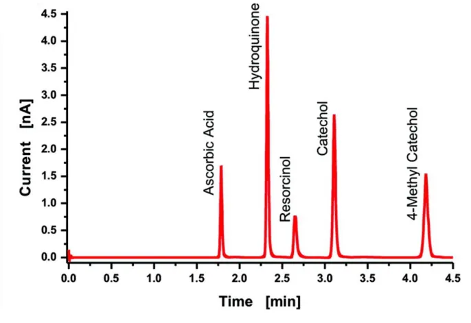
electrochemical test mixture on the capillary LC evaluation system with carbon microfiber electrochemical detection. This run was conducted at 460 bar (1.9 mm/s, v = 4) with a mobile phase of 50:50 (v/v)

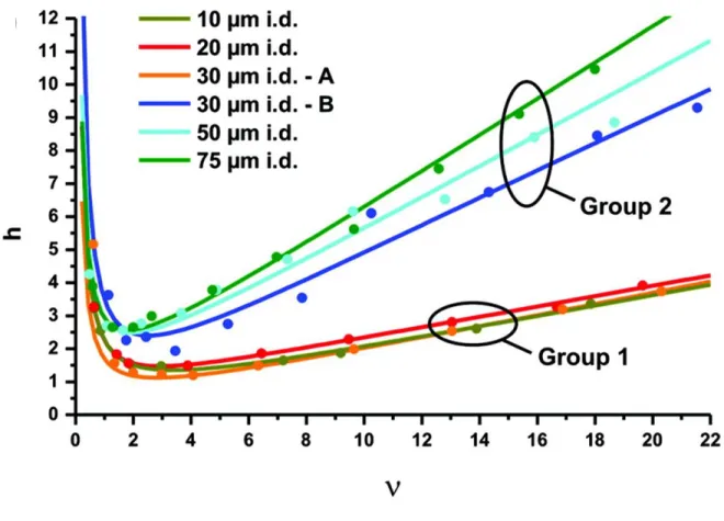
water:acetonitrile with 0.1% TFA. ... 49 Figure 2-8. Set of h-v curves for six capillary LC columns (~20 cm, of inner

diameters shown) packed with 1.9 μm BEH particles. Solid lines of the same color indicate a best fit to Equation 2-8 for each column. Group 1 indicates columns of good (expected) performance while Group 2

indicates columns of poorer performance. ... 50 Figure 2-9. Full reconstruction model of a 30 μm i.d. capillary column packed

with 1.9 μm BEH particles. The reconstruction is made up of 6,967 fitted

particles over a length of 65 μm... 51 Figure 2-10. Color-coded 2-D porosity (interparticle void volume fraction) profile

of a 30 μm i.d. column packed with 1.9 μm BEH particles. Warmer colors

indicate higher porosity and cooler colors indicate lower porosity. ... 52 Figure 2-11. Radial porosity (interparticle void volume fraction) profiles for six

capillary LC columns (of inner diameters shown) packed with 1.9 μm BEH particles. Group 1 indicates columns of good (expected)

performance while Group 2 indicates columns of poorer performance. ... 53 Figure 2-12. Porosity deviation plot used to calculate the IPD value for a 20 μm

i.d. column packed with 1.9 μm BEH particles, representative of the

Group 1 (good performing) columns. ... 54 Figure 2-13. Porosity deviation plot used to calculate the IPD value for a 75 μm

i.d. column packed with 1.9 μm BEH particles, representative of the

Group 2 (poorer performing) columns. ... 55 Figure 2-14. Measure of the mean particle size plotted as a function of the

distance from the capillary wall for six capillary LC columns (of inner

diameters shown) packed with 1.9 μm BEH particles. ... 56

Figure 2-15. Visual depiction of particle size positions in a 30 μm i.d. column packed with 1.9 μm BEH particles. Particles in the lowest 25% of of the PSD of the 3-D reconstruction are highlighted in yellow. Particles in the

highest 25% of the PSD of the 3-D reconstruction are highlighted in blue. ... 57 Figure 2-16. Visual depiction of particle size positions in a 75 μm i.d. column

packed with 1.9 μm BEH particles. Particles in the lowest 25% of the PSD of the 3D reconstruction are highlighted in yellow. Particles in the

highest 25% of the PSD of the 3-D reconstruction are highlighted in blue. ... 58 Figure 2-17. Comparison of local particle size distribution and global particle

(15)

wall and 13 particle diameters from the column wall) for a 75 μm i.d.

column packed with 1.9 μm BEH particles. ... 59 Figure 2-18. h-v curves of hydroquinone for 75 μm i.d. columns (~20 cm) packed

with 1.9 μm BEH particles at slurry concentrations of 3 mg/mL and 100

mg/mL. Mobile phase was 50:50 (v/v) water:acetonitrile with 0.1% TFA. ... 60 Figure 2-19. h-v curves of hydroquinone for 50 μm i.d. columns (~20 cm) packed

with 1.7 μm BEH particles at slurry concentrations of 3 mg/mL and 30

mg/mL. Mobile phase was 50:50 (v/v) water:acetonitrile with 0.1% TFA. ... 61 Figure 2-20. Restored CLSM images of 1.9 μm BEH particles packed into a 75

μm i.d. column (100 mg/mL slurry concentration) and 1.7 μm BEH particles packed into a 50 μm i.d. column (30 mg/mL slurry

concentration). ... 62 Figure 2-21. Radial porosity (interparticle void volume fraction) profiles for 75

μm i.d. columns packed with 1.9 μm BEH particles at 3 and 100 mg/mL slurry concentrations and 50 μm i.d. columns packed with 1.7 μm BEH

particles at 3 and 30 mg/mL slurry concentrations. ... 63 Figure 2-22. Measure of the mean particle size plotted as a function of the

distance from the capillary wall for six capillary LC columns (of inner

diameters shown) packed with 1.9 μm BEH particles. ... 64 Figure 3-1. Representation of the surface-restricted molecular diffusion model,

where Qstis the isosteric heat of adsorption and Es is the activation energy of surface diffusion. Adapted with permission from Miyabe, K. Journal of

model for particle-packed beds (A) and monolithic columns (B). ... 84 Figure 3-3. Variance vs. stop time plots for 2.1 x 50 mm BEH and Chromolith

columns run in gradient mode. Peak variance is measured for the renin substrate (DRVYIHPFHLLVYS) peak detected (at 214 nm) from the Waters MassPREP Peptide Mixture. For the BEH column, the sample was loaded at 1%B, run from 1-5%B over one minute and held for a selected stop time (0 min, 2 min, 2 hr, 8 hr, and ~30 hr), then run from 5-50%B over 9 minutes. For the Chromolith column, the sample was loaded at 5%B, run for 1 minute and held for a selected stop time (0 min, 10 min, and 24 hr), then run from 5-50%B over 10 minutes. (100 μL/min for all separations, A: optima-grade water with 0.1% trifluoroacetic acid, B: optima-grade acetonitrile with 0.1% trifluroacetic acid). Dotted lines to

(16)

valerophenone. For the BEH column the mobile phase was 78/22 (v/v) water/acetonitrile (k’ ≈ 98) and for the Chromolith column the mobile

phase was 82/18 (v/v) water/acetonitrile (k’ ≈ 93). ... 86

Figure 3-5.Mobile phase and stationary phase diffusion coefficients calculated for valerophenone on a 2.1 x 50 mm BEH column tested at a series of

retention factors for a four-hour stop time. Mobile phase diffusion coefficients were calculated by the Wilke-Change Equation (Equation 3-24e) and Ds was calculated with Equation 3-24f. Increased k’ values were obtained by decreasing the acetonitrile fraction in the water/acetonitrile

mobile phase (50%, 35%, 27%, and 22%, respectively). ... 87 Figure 3-6. Ds/Dm vs. retention factor plot for valerophenone on a 2.1 x 50 mm

BEH column tested at a series of retention factors for a four-hour stop

time based on values from Figure 3-5... 88 Figure 3-7. Diffusion coefficient ratio vs. retention factor plot tested at a series of

retention factors. UNC data is adapted from Figure 3-6 while monolith and 5 μm C18 particle data is adapted with permission from Miyabe, K.

Oxford University Press. ... 89 Figure 3-8. Plot of the logarithm of Ds/Dm vs. the logarithm of the inverse of the

retention factor for valerophenone on a 2.1 x 50 mm BEH column tested at a series of retention factors for a four-hour stop time based on values from

Figure 3-5. ... 90 Figure 3-9. Reduced b-term vs. k’ on a 18.9 cm x 30 μm i.d. column packed with

0.9 μm BEH particles. k' was reported for four compounds

(hydroquinone, resorcinol, catechol, and 4-methyl catechol) at five

different mobile phase compositions (20, 30, 50, 70, and 80%B). The red dashed line displays Equation 3-25f when χ ≈ 2. Adapted with permission from Lieberman, R. A. UNC Doctoral Dissertation, 2009. Copyright 2009

Rachel A. Lieberman. ... 91 Figure 4-1. Representation of a perfusion chromatography particle. Adapted with

permission from Afeyan, N. B., Gordon, N. F., Mazsaroff, I., Varady, L., Fulton, S. P., Yang, Y. B., Regnier, F. E. Journal of Chromatography,

morphologies: macroporous (green), hybrid (or Janus, yellow), and

mesoporous (red). ... 115 Figure 4-4. Chromatogram of a mixture of four electrochemically active analytes

(17)

catechol (4MC)) run on a 19 cm x 75 μm i.d. capillary column packed with 1.2 μm (nominally) USP particles bonded with C18. The mobile phase was 80/20 (v/v) water/acetonitrile with 0.1% trifluoroacetic acid and the inlet pressure was 22 kpsi. Measured plate counts (N) are shown for

each peak. ... 116 Figure 4-5. H-u curve of hydroquinone measured on a 19 cm x 75 μm i.d.

capillary column packed with 1.2 μm (nominally) USP particles bonded with C18. The mobile phase was 80/20 (v/v) water/acetonitrile with 0.1%

trifluoroacetic acid. Inlet pressures ranged from 7.9 to 38 kpsi... 117 Figure 4-6. Flow resistance comparison of a 19 cm x 75 μm i.d. capillary column

packed with 1.2 μm (nominally) USP particles bonded with C18 to theoretical curves for columns of the same dimensions packed with 0.5, 1.0, and 1.5 μm porous (assumed εi = 0.4 and εt = 0.7) particles calculated

by the Kozeny-Carman equation (Equation 1-32). ... 118 Figure 4-7. Depiction of hydrodynamic chromatography of two particles in a

capillary tube where rc represents the capillary radius and rp represents the particle radius (rp,1 > rp,2). Adapted with permission from Striegel, A. M., Brewer, A. K., Annual Review of Analytical Chemistry, 2012, 5, 15-34.

standards (urea dead time marker in each run) with 0.2, 1.2, and 5.0 mg/mL sample concentrations, respectively. The glass HDC column was 86 cm x 10 mm diameter packed with 34 μm glass beads, run at 4 mL/min

in 1 mM ammonium hydroxide mobile phase. ... 120 Figure 4-9. SEM images of the HDC polyethylene frit (A), a zoomed-in image of

the polyethylene frit showing trapped silica particles (B), and the

replacement stainless steel mesh frit (C). ... 121 Figure 4-10. Separation of 0.5 and 1.5 μm NPS spheres (with urea dead time

marker) on two 10 mm diameter HDC columns of different lengths packed with 34 μm glass beads. The red trace is for a 47 cm long column and the blue trace is for a 86 cm (39 cm packed on top of the 47 cm column) long column. Both runs were conducted at 4 μL/min (1 mM ammonium hydroxide mobile phase), so the 47 cm column data has been scaled

(based on the ratio of column dead times). ... 122 Figure 4-11. HDC chromatogram for the separation of 0.5 and 1.5 μm silica size

standards (with an added urea dead time marker). The glass HDC column was 86 cm x 10 mm diameter packed with 34 μm glass beads, run at 4

(18)

column was 86 cm x 10 mm diameter packed with 34 μm glass beads, run

at 4 mL/min in 1 mM ammonium hydroxide mobile phase. ... 124 Figure 4-13. HDC chromatogram for the refinement of 1.0 μm BEH particles. 1

mg was injected (100 μL of a 10 mg/mL slurry) and four fractions (12 s each) were collected across the peak. The glass HDC column was 86 cm x 10 mm diameter packed with 34 μm glass beads, run at 4 mL/min in 1

mM ammonium hydroxide mobile phase. ... 125 Figure 4-14. A series of ten consecutive injections (at each dotted line, 4 minutes

apart) of the separation shown in Figure 4-13. ... 126 Figure 4-15. Histograms representing ~100 particles sized by SEM for each HDC

fraction collected in Figure 4-13. Average size values (reported with one standard deviation) are: 1.0 μm BEH starting material (A): 1.02 ± 0.24 μm; Fraction 1 (B): 1.24 ± 0.18 μm; Fraction 2 (C): 1.13 ± 0.18 μm;

Fraction 3 (D): 0.98 ± 0.16 μm; and Fraction 4 (E): 0.88 ± 0.15 μm. ... 127

Figure 4-16. HDC chromatogram for the refinement of 1.2 μm USP particles. 1 mg was injected (100 μL of a 10 mg/mL slurry) and two fractions (30 s each) were collected across the peak. The glass HDC column was 86 cm x 10 mm diameter packed with 34 μm glass beads, run at 4 mL/min in 1

mM ammonium hydroxide mobile phase. ... 128 Figure 4-17. Comparison of the particle size distributions of Fractions 1 and 2

collected in Figure 4-16 to the raw (pre-refined) 1.2 μm USP material. The percentage of macroporous, hybrid, and mesoporous particles are shown for each fraction and the average size (± 1 standard deviation) for each particle type. The average particle sizes (for the total fraction) are: 1.23 ± 0.23 μm (Fraction 1), 1.25 ± 0.37 μm (Raw), and 0.97 ± 0.21 μm

(Fraction 2)... 129 Figure 4-18. Comparison of the particle size distributions of the raw 1.2 μm USP

material to material collected following two separate steps of HDC refinement. The percentage of macroporous, hybrid, and mesoporous particles are shown for each fraction and the average size (± 1 standard deviation) for each particle type. The average particle sizes (for the total fraction) are: 1.25 ± 0.37 μm (30% RSD, Raw), 1.23 ± 0.23 μm (19%

RSD, Refinement 1), and 1.25 ± 0.17 μm (14% RSD, Refinement 2). ... 130 Figure 4-19. SEM images of the unrefined, raw 1.2 μm USP particles and the

same particles following two refinement steps by HDC. ... 131 Figure 5-1. Electron micrographs of 1.8 μm HSS particles (A) and 1.5 μm SPP

particles (B). ... 159 Figure 5-2. Mini hypodermic thermocouple probe HYP-0 (A) attached to an

(19)

(C). Diagram of the thermocouple probe inserted into PEEK tubing at the

outlet of a standard-bore LC column is shown in (D). ... 160 Figure 5-3. Diagram of a standard-bore LC column held within an external sleeve

designed to contain particulate insulation (aerogel). ... 161 Figure 5-4. Diagram of a standard-bore LC column held within a water

flow-through cell. ... 161 Figure 5-5. Temperature change values measured using a hypodermic

thermocouple probe at the outlet of 2.1 x 50 mm BEH and SPP columns in acetonitrile at 10, 250, 500, 750, 1,000, 1,250, and 1,500 μL/min for 20

minutes each (with a final 20 minute period back at 10 μL/min). ... 162

Figure 5-6. Comparison of measured and extra-column band broadening corrected efficiency values of hexadecanophenone on a 2.1 x 50 mm SPP column

(acetonitrile mobile phase). ... 163 Figure 5-7. h-v curves for hexadecanophenone in acetonitrile mobile phase on 2.1

x 50 mm HSS and SPP columns (corrected for extra-column band

broadening). ... 164 Figure 5-8. Temperature change values (measured using a hypodermic

thermocouple probe at the column outlet) compared to generated power

for 2.1 x 50 mm diameter HSS and SPP columns. ... 165 Figure 5-9. k’ measured for hexadecanophenone in acetonitrile on 2.1 x 50 mm

BEH, HSS, and SPP columns at flow rates ranging from 25 μL/min to

1,600 μL/min (maximum flow rate based on pressure limitations). ... 166 Figure 5-10. Comparison of measured and extra-column band broadening

corrected efficiency values of hexadecanophenone on a 2.1 x 150 mm

HSS column (acetonitrile mobile phase). ... 167 Figure 5-11. h-v curves for hexadecanophenone in acetonitrile mobile phase on

2.1 mm diameter HSS columns of 5 and 15 cm length (corrected for

extra-column band broadening). ... 168 Figure 5-12. Temperature change values (measured using a hypodermic

for 2.1 x 50 mm diameter HSS columns of 5 and 15 cm length. ... 169 Figure 5-13. k’ measured for hexadecanophenone in acetonitrile on on 2.1 mm

(20)

Figure 5-14. Comparison of measured and extra-column band broadening corrected efficiency values of hexadecanophenone on a 1.0 x 150 mm

HSS column (acetonitrile mobile phase). ... 171 Figure 5-15. h-v curves for hexadecanophenone in acetonitrile mobile phase on 15

cm HSS columns of 1.0 and 2.1 mm diameter (corrected for extra-column

band broadening). ... 172 Figure 5-16. Temperature change values (measured using a hypodermic

for 15 cm HSS columns of 1.0 and 2.1 mm diameter. ... 173 Figure 5-17. k’ measured for hexadecanophenone in acetonitrile on 15 cm HSS

columns of 1.0 and 2.1 mm diameter at flow rates ranging from 25 μL/min

to 900 μL/min (maximum flow rate based on pressure limitations). ... 174 Figure 5-18. h-v curves for hexadecanophenone in acetonitrile mobile phase on

2.1 x 150 mm HSS columns in the standard Acquity instrument column oven, inside an insulation jacket filled with aerogel (adiabatic), and inside a jacket that allows for heat transfer by water flow (corrected for

extra-column band broadening). ... 175 Figure 5-19. Temperature change values (measured using a hypodermic

thermocouple probe at the column outlet) compared to generated power for 2.1 x 150 mm HSS columns in still air (representative of the Acquity instrument column oven), inside an insulation jacket filled with aerogel,

and inside a jacket that allows for heat transfer by water flow. ... 176 Figure 5-20. k’ measured for hexadecanophenone in acetonitrile on 2.1 x 150 mm

HSS columns in the standard Acquity instrument column oven, inside an insulation jacket filled with aerogel, and inside a jacket that allows for heat transfer by water flow length at flow rates ranging from 50 μL/min to

900 μL/min. ... 177

Figure 5-21. h-v curves for hexadecanophenone in acetonitrile mobile phase on 2.1 x 150 mm HSS and SPP columns in the standard Acquity instrument column oven and inside a jacket that allows for heat transfer by water flow

(corrected for extra-column band broadening). ... 178 Figure 5-22. Temperature change values (measured using a hypodermic

thermocouple probe at the column outlet) compared to generated power for 2.1 x 150 mm HSS and SPP columns in still air (representative of the Acquity instrument column oven) and inside a jacket that allows for heat

transfer by water flow. ... 179 Figure 5-23. k’ measured for hexadecanophenone in acetonitrile on 2.1 x 150 mm

(21)

and inside a jacket that allows for heat transfer by water flow at flow rates

ranging from 50 μL/min to 900 μL/min. ... 180 Figure 5-24. Gradient separation of the Waters MassPREP Peptide Mixture (6 μL

injected) on a 2.1 x 150 mm HSS column. The black trace is the raw, measured data, the dotted green trace indicates the UV signal acquired when the gradient is run with no sample injection, and the red trace is the baseline corrected chromatogram. Gradient conditions were 1-50%B (A: optima-grade water with 0.1% trifluoroacetic acid, B: optima-grade

acetonitrile with 0.1% trifluoroacetic acid) over 30 minutes (100 μL /min). ... 181 Figure 5-25. Range for peak capacity measurements where the gradient time is

calculated from Peak 1 to Peak 6 and the peak widths are averaged from

all 6 peaks. Peak identifications can be found in Table 5-2... 182 Figure 5-26. Gradient separation (1-50%B, A: optima-grade water with 0.1%

trifluoroacetic acid, B: optima-grade acetonitrile with 0.1% trifluoroacetic acid) of the Waters MassPREP Peptide Mixture (6 μL injected) on a 2.1 x 150 mm HSS column at three different flow rates: 100 μL/min (30

minutes, red trace), 200 μL/min (15 minutes, black trace), and 300 μL/min

(10 minutes, blue trace)... 183 Figure 5-27. Peak capacities (calculated by Equation 5-5) for 2.1 mm diameter

HSS and SPP columns of 5 and 15 cm length. ... 184 Figure 5-28. Temperature change values (measured using a hypodermic

for 2.1 mm diameter HSS and SPP columns of 5 and 15 cm length. ... 185 Figure 6-1. Graphical plot of Equation 6-11 with a sigma value of 0.2 s, Apeak set

to 1, tr equal to 10 s, and tau values of 0.1, 0.3, 0.5, and 1.0 s. ... 210 Figure 6-2. Diagram (not-to-scale) of instrument set-up used to test open-tube

broadening using the subtraction method (including inset showing internal

capillary butt connection inside the zero-dead volume union). ... 211 Figure 6-3. Valve diagram for the four-port internal sample loop Valco injector.

Red sections indicate fluid that contains analyte while blue indicates

mobile phase. ... 212 Figure 6-4. Diagram (not-to-scale) of instrument set-up used to test open-tube

broadening using the direct measurement method. ... 213 Figure 6-5. 3-D axisymmetric model of the injector (rotor and stator) connected to

(22)

Figure 6-6. Photographs of a prototype titanium substrate LC tiles manufactured by Waters Corporation and prototype tile-to-capillary fittings used with the tile. A tile with three straight channels is shown in A (channel position overlaid in blue). Different fittings used for making capillary connections

to and from the tile are shown separately in B and installed in C. ... 215 Figure 6-7. Diagram (not-to-scale) of instrument set-up used to test packed LC

tile column performance with UV detection. ... 216 Figure 6-8. Variance values measured using the subtraction method for nominally

25, 30, 40, and 50 μm i.d. capillaries (1 m long) at flow rates ranging from

0.5 – 14 μL/min. ... 217 Figure 6-9. Measurement of 4-methyl catechol through a 6 cm, 13 μm i.d.

capillary using a carbon fiber electrode detector with a full loop injection. Data acquisition rate was set at 80 Hz and preamplifier filter rates were set

to 3, 10, and 30 Hz. ... 218 Figure 6-10. Variance values measured using the direct measurement method with

a full loop injection for 21, 29, 42, and 51 μm i.d. capillaries (1 m long) at

flow rates ranging from 0.5 – 15 μL/min. ... 219 Figure 6-11. Representation of fluid containing analyte (red) moving from the

internal loop into the connecting capillary when switched into inject mode (mobile phase in blue). The dotted line separates the part of the sample that does not enter the capillary during a timed pinch injection. Adapted with permission from Foster, M. D., Arnold, M. A., Nichols, J. A., Bakalyar, S. R. Journal of Chromatography A, 2000, 869, 231-241.

a timed pinch injection for 21, 29, 42, and 51 μm i.d. capillaries (1 m long)

at flow rates ranging from 0.5 – 15 μL/min. ... 221 Figure 6-13. Variance values calculated using an EMG peak fit and an ISM

algorithm (interval of -3σ, +5σ) for a 1 m, 20 μm i.d. capillary with a

timed pinch injection... 222 Figure 6-14. Sigma-squared values measured using the direct measurement

method with both full loop and timed pinch injections for 21, 29, 42, and 51 μm i.d. capillaries (1 m long) at flow rates ranging from 0.5 – 15 μL/min. Straight lines indicate values calculated using Taylor-Aris theory

(Equation 6-6). ... 223 Figure 6-15. Tau-squared values measured using the direct measurement method

with a full loop injection for 21, 29, 42, and 51 μm i.d. capillaries (1 m

(23)

Figure 6-16. Tau-squared values measured using the direct measurement method with a timed pinch injection for 21, 29, 42, and 51 μm i.d. capillaries (1 m

long) at flow rates ranging from 0.5 – 15 μL/min. ... 225 Figure 6-17. COMSOL modeling of analyte moving from a 20 nL internal loop

through the instrument stator (100 μm i.d.) and into 2.5 mm of a 29 μm i.d. capillary. Red regions represent the initial analyte concentration (conc. = 1) and blue regions represent the mobile phase (conc. = 0) with a colored gradient in between. Flow rate is 15 μL/min and time points are 0,

0.025, 0.05, 0.075, and 0.1 s. ... 226 Figure 6-18. Comparison of τ2 values (29 μm i.d.) from the 3-D axisymmetric

COMSOL model (Model 1, just the injector), combined 2-D and 3-D axisymmetric COMSOL model (Model 2, injector and tube), and

experimental data from Figure 6-15 (injector and tube). ... 227 Figure 6-19. Peak injection profiles of a full loop injection measured out of the

injector through a small (6 cm, 13 µm inner diameter) connecting capillary

for eight flow rates between 0.5 and 15 μL/min. ... 228 Figure 6-20. Peak injection profiles of a timed pinch injection measured out of the

injector through a small (6 cm, 13 µm inner diameter) connecting capillary

for eight flow rates between 0.5 and 15 μL/min. ... 229 Figure 6-21. Expanded peak injection profiles of a timed pinch injection measured

out of the injector through a small (6 cm, 13 µm inner diameter)

connecting capillary for six flow rates between 4 and 15 μL/min. ... 230 Figure 6-22. Comparison of full loop and timed pinch peak injection profiles

measured out of the injector through a small (6 cm, 13 µm inner diameter)

connecting capillary at 10 μL/min. ... 231 Figure 6-23. Standard chromatogram from a 300 μm i.d. titanium tile packed with

1.8 μm HSS particles using a 5-compound test mixture (uracil,

acetophenone, propiophenone, butyrophenone, and valerophenone) with UV detection. Mobile phase was 50:50 (v/v) water:acetonitrile with 0.1%

TFA. ... 232 Figure 6-24. van Deemter curves measured for acetophenone (red, k’ = 1.4) and

butyrophenone (blue, k’ = 4.3) on a 10 cm, 300 μm i.d. titanium tile column packed with 1.8 μm HSS particles. Raw data is shown is shown with the filled circles (fit to Equation 1-20 with solid lines) and ECBB corrected values are shown with the open circles (fit to Equation 1-20 with

(24)

LIST OF ABBREVIATIONS

2-D Two-dimensional

3-D Three-dimensional

4MC 4-methyl catechol

AA Ascorbic acid

BEH Bridged-ethyl hybrid BJH Barrett-Joyner-Halenda

C18 n-Octadecyl

CAT Catechol

CFD Computational fluid dynamics CLSM Confocal laser scanning microscopy DMSO Dimethyl sulfoxide

ECBB Extra-column band broadening EMG Exponentially-modified Gaussian EMT Effective medium theory

FPP Fully porous particle

HDC Hydrodynamic chromatography HETP Height equivalent to a theoretical plate HPLC High pressure liquid chromatography HSS High strength silica

HQ Hydroquinone

IPD Integral porosity deviation

(25)

i.d. Inner diameter

LC Liquid chromatography

LC-MS Liquid chromatography-Mass spectrometry

MeCN Acetonitrile

MoM Method of (statistical) moments

NPS Nonporous silica

o.d. Outer diameter

PE Polyethylene

PEEK Polyether ether ketone PSD Particle size distribution PS-DVB Poly(styrene-divinyl benzene) PTFE Polytetrafluoroethylene

RES Resorcinol

RSD Relative standard deviation SEM Scanning electron microscopy SPP Superficially porous particle

SS Stainless steel

TEM Transmission electron microscopy TFA Trifluoroacetic acid

TTL Through-the-Lens

(26)

UV Ultraviolet

(27)

LIST OF SYMBOLS

A Multiple flow path van Deemter coefficient

Apeak Peak amplitude

a Reduced multiple flow path van Deemter coefficient

aKnox Reduced multiple flow path van Deemter coefficient in the Knox model

B Longitudinal diffusion van Deemter coefficient

Bm Longitudinal diffusion in the mobile phase van Deemter coefficient

Bs Longitudinal diffusion in the stationary phase van Deemter coefficient %B Percentage of organic modifier in the mobile phase (for either isocratic or

gradient separations)

b Reduced longitudinal diffusion van Deemter coefficient

bKnox Reduced longitudinal diffusion van Deemter coefficient in the Knox model

C Reduced resistance to mass transfer van Deemter coefficient

CHDC Hydrodynamic chromatography quadratic correction term

Cm Resistance to mass transfer in the mobile phase van Deemter coefficient

Cs Resistance to mass transfer in the mobile phase van Deemter coefficient

Csm Resistance to mass transfer in the stagnant mobile phase van Deemter coefficient

c Resistance to mass transfer van Deemter coefficient

cKnox Reduced resistance to mass transfer van Deemter coefficient in the Knox model

cs Particle slurry concentration

(28)

Deff,s Effective diffusion coefficient in the stationary phase

Dm Diffusion coefficient in the mobile phase

Dm,0 Frequency factor of molecular diffusion in the mobile phase

Dmz Diffusion coefficient in the mobile zone

Dpore Diffusion coefficient in the particle pores

Ds Diffusion coefficient in the stationary phase

Ds,0 Frequency factor of molecular diffusion in the stationary phase

Dsz Diffusion coefficient in the stationary zone

dm Theoretical microparticle diameter

dp Particle diameter

dp,HDC Hydrodynamic chromatography packing material particle diameter

dp,n Number-averaged particle diameter

dp,vol Volume-averaged particle diameter

dpore Pore diameter

ds Stationary phase film thickness

Em Activation energy of molecular diffusion in the mobile phase

Es Activation energy of molecular diffusion in the stationary phase

Evap Energy of evaporation

F Flow rate

ffilt Detector filter cutoff frequency

f(t) Measured peak signal in the time domain

G Gradient compression factor

(29)

H Height equivalent to a theoretical plate

HA Height equivalent to a theoretical plate due to multiple flow path broadening

HA,Giddings Height equivalent to a theoretical plate due to multiple flow path

broadening in the Giddings model

HB Height equivalent to a theoretical plate due to longitudinal diffusion

HB,m Height equivalent to a theoretical plate due to longitudinal diffusion in the mobile phase

HB,s Height equivalent to a theoretical plate due to longitudinal diffusion in the stationary phase

HC Height equivalent to a theoretical plate due to resistance to mass transfer

HC,m Height equivalent to a theoretical plate due to resistance to mass transfer in the mobile phase

HC,s Height equivalent to a theoretical plate due to resistance to mass transfer in the stationary phase

HC,sm Height equivalent to a theoretical plate due to resistance to mass transfer in the stagnant mobile phase

Hmin Minimum height equivalent to a theoretical plate

h Reduced height equivalent to a theoretical plate

ha Reduced height equivalent to a theoretical plate due to multiple flow path broadening

ha,Giddings,i Reduced height equivalent to a theoretical plate due a multiple flow path

broadening mechanism i in the Giddings model

hads Reduced height equivalent to a theoretical plate due to slow adsorption-desorption kinetics in the Gritti-Guiochon model

hb Reduced height equivalent to a theoretical plate due to longitudinal diffusion

(30)

hGiddings Reduced height equivalent to a theoretical plate in the Giddings model

hKnox Reduced height equivalent to a theoretical plate in the Knox model

hlong Reduced height equivalent to a theoretical plate due to longitudinal diffusion in the Gritti-Guiochon model

hmin Minimum reduced height equivalent to a theoretical plate

hmt,m Reduced height equivalent to a theoretical plate due to resistance to mass transfer in the mobile phase in the Gritti-Guiochon model

hmt,s Reduced height equivalent to a theoretical plate due to resistance to mass transfer in the stationary phase in the Gritti-Guiochon model

htc Transcolumn reduced height equivalent to a theoretical plate in the Gritti-Guiochon model

htotal Total reduced height equivalent to a theoretical plate in the

Gritti-Guiochon model

Ka Adsorption equilibrium constant

Ka,0 Frequency factor of adsorption equilibrium

Kbed Specific permeability constant of a packed bed

Kpart Specific permeability constant of a particle

kads Adsorption rate constant

kB Boltzmann constant

k' Retention factor

k’0 Retention factor at initial gradient condition

k’g Gradient retention factor

k’part Particle retention factor

L Column length

MA Solute molecular weight

(31)

N Number of theoretical plates

nc Peak capacity

ΔP Pressure drop across the column

Qst Isosteric heat of adsorption

R Universal gas constant

Rs Resolution

rc Column (or capillary) radius

rc,HDC Interstitial capillary radius in a particle-packed hydrodynamic

chromatography column

rp Particle radius

rsolid-core Solid-core radius (in a superficially porous particle)

S Retention and organic solvent concentration relationship constant

T Temperature

ΔTL Axial temperature change ΔTR Radial temperature change

t Time

t0 Column void (dead) time

tfilt Detector filter time constant

tG Gradient time length

tin Time into the stationary phase

tm Time analyte spends in mobile phase

tmix Mean time an analyte spends in a mixing chamber

(32)

tr Analyte retention time

ts Time analyte spends in stationary phase

tsamp Detector sampling time (inverse data acquisition rate)

u Mobile phase velocity

ui Interstitial mobile phase velocity

up Particle velocity in hydrodynamic chromatography

ur Local velocity at radial position r

us Sedimentation velocity

umeas Measured mobile phase velocity

upore Mobile phase velocity through particle pores

VA Solute molar volume

Vdet Detector volume

Vf Solvent free volume

Vinj Injection volume

Vsp Specific pore volume

w Peak basewidth

wavg Mean peak basewidth

α Relative retention

αT Thermal expansion coefficient of the solvent

β Surface diffusion fractional isosteric heat of adsorption

βlong Effective medium theory diffusion coefficient ratio term

γ Tortuosity (obstruction) factor

(33)

γs Tortuosity (obstruction) factor in the stationary phase

γsm Tortuosity (obstruction) factor in the stagnant mobile phase

δi Thermal conductivity of component i

δMeCN Thermal conductivity of acetonitrile

δm Thermal conductivity of a medium

δp Thermal conductivity of the packed bed (including solvent)

δwater Thermal conductivity of water

ε(r) Local interstitial porosity at radial position r from the column center

εbulk Interstitial porosity in the bulk packing region

εi Interstitial porosity

εpp Intraparticle porosity

εsk Particle skeleton fraction

εt Total column porosity

ζ Cm-term packed bed structure coefficient

η Mobile phase viscosity

κ Ratio of pore velocity to total mobile phase velocity

λA A-term packed bed structure coefficient

λdiff Distance between two neighboring equilibrium positions in diffusion

λHDC Ratio of particle radius to capillary radius in hydrodynamic chromatography

λi Advection structural parameter in the Giddings model

(34)

λtch Transchannel advection structural parameter in the Giddings model

v Reduced mobile phase velocity

v1/2,i Reduced transition velocity of a given broadening contribution i in the

Giddings model

v1/2,sr Reduced transition velocity of the short-range interchannel contribution in

the Giddings model

v1/2,tc Reduced transition velocity of the transcolumn contribution in the

Giddings model

v1/2,tch Reduced transition velocity of the transchannel contribution in the

Giddings model

vopt Optimum reduced mobile phase velocity

ξlong Torquato model parameter

ρ Ratio of solid core radius to total particle radius in a superficially porous particle

ρliq Solvent density

ρsk Particle skeletal density

σfit Sigma parameter from the Exponentially-modified Gaussian peak fit

σ2

det Sigma-type variance contribution from the detector

σ2

diff Variance due to longitudinal molecular diffusion

σ2

diff,l Spatial variance due to longitudinal molecular diffusion

σ2

diff,time Temporal variance due to longitudinal molecular diffusion

σ2

inj Sigma-type variance contribution from the injector

σ2

l Spatial variance

σ2

time Temporal variance

σ2

tot,sys Total system (extra-column) variance

σ2

(35)

σ2

var,EMG Peak variance calculated using the Exponentially-modified Gaussian

peak-fitting technique

σ2

var,MOM Peak variance calculated using the statistical moments method

σ2

vol Volumetric variance

σ2

vol,det Sigma-type volumetric variance contribution from the detector

σ2

vol,inj Sigma-type volumetric variance contribution from the injector

σ2

vol,tube Sigma-type volumetric variance contribution from connecting tubing

τdiff Diffusion rate constant

τfit Tau parameter from the Exponentially-modified Gaussian peak fit

τHDC Hydrodynamic chromatography particle elution factor

τ2

data Tau-type variance contribution from the data acquisition rate

τ2

filt Tau-type variance contribution from the detector filter rate

τ2

flow Tau-type variance contribution from mixing volumes

τ2

time,chmbr Tau-type temporal variance contribution from a diffusion chamber

τ2

time,data Tau-type temporal variance contribution from the data acquisition rate

τ2

time,filt Tau-type temporal variance contribution from the detector filter rate

τ2

time,mix Tau-type temporal variance contribution from a mixing chamber

Δϕ Change in fraction of organic modifier in the mobile phase

ϕm,i Volume fraction of component i in a medium

φ Stagnant mobile phase fraction

χ Surface-restricted molecular diffusion model constant

ΨB Solvent association factor

(36)

ωsr Short-range interchannel diffusion structural parameter in the Giddings model

ωtc Transcolumn diffusion structural parameter in the Giddings model

ωtch Transchannel diffusion structural parameter in the Giddings model

ωα,i Distance an analyte molecule must travel by advection to encounter all possible velocity paths for a given broadening contribution i in the Giddings model

ωα,tc Distance an analyte molecule must travel by advection to encounter all possible velocity paths for the transcolumn contribution in the Giddings model

ωβ,i Ratio of the velocity extremes across the range of a given broadening contribution i to the mean velocity across this range in the Giddings model

ωβ,tc Ratio of the velocity extremes across the range of the transcolumn broadening contribution to the mean velocity across this range in the Giddings model

(37)

CHAPTER 1. Introduction to Band Broadening Theory

1.1 Overview

High pressure liquid chromatography (HPLC) is one of the most ubiquitous and important analytical techniques in use today.1,2 According to a recent strategic business report on HPLC systems and accessories prepared by Global Industry Analysts, Inc., the global liquid chromatography (LC) market will expand to nearly $5 billion by the year 2020.3 As the field continues to grow and the worldwide user base expands, improving the performance and speed of this technique is paramount for continued growth. The most vital factor in a separation by LC (and the focus of this thesis) is the column1,2, where further development is one of the keys to achieving these improvements. In this introduction, the general theory of band broadening in LC columns will be described in order to present readers with the necessary background to

understand the research presented here. More recent developments in the field focused on ultra-high pressure liquid chromatography (UHPLC) that have impacted LC column (and instrument) research will also be detailed. The specific sections relevant to each chapter in the thesis will be detailed throughout the rest of this introduction.

1.2 Band Broadening Theory

1.2.1 The Basics of Separations and Separation Terminology

(38)

terminology relates this spatial variance to a factor referred to as the height equivalent to a theoretical plate (HETP, or H) through the column length (L)4:

L

H l

2 

 (1-1)

The number of theoretical plates in a column (N) is a measure of separation efficiency and is a ratio of the total column length to one HETP1:

2 2 l L H L N  

 (1-2)

In nearly all cases, chromatograms are measured in the time domain, so N can also be described in terms of temporal variance (σtime2)1:

2 2 time r t N   (1-3)

where tr is the analyte retention time, or the amount of time spent on the column. The retention time is the sum of time an analyte spends in the stationary (ts) and mobile (tm) phases:

m s r t t

t   (1-4)

tm is the time it takes for the entire mobile phase fraction to elute from the column and is also referred to as the column dead time (t0) which is interchangeable with tm and can be measured by the elution time of a non-retained analyte.2 The most popular form of LC (reversed phase LC) consists of a particulate material (usually spherical silica) coated with a thin hydrophobic stationary phase layer (this material is then packed into a column) and mobile phases that are mixtures of water and an organic solvent (typically acetonitrile or methanol). It is the

(39)

0 0 ' t t t t t k r m

s  

 (1-5)

Resolution (Rs) is the term used to describe the separation between two analytes and is related to both N and k’1:

1 ' ' 1 4 ₂ 2      k k N R_s   (1-6)

where α is the relative retention (the ratio of the two retention factors, k’2/k’1). To quickly determine resolution from a measured chromatogram, the following formula based on the peak basewidths (w, which is equal to 4σt) can be used1:







1 2



1 , 2 , 2 w w t t

Rs r r

 

 (1-7)

1.2.2 van Deemter Theory

Every process that broadens a band has its own variance contribution. If these processes are independent from each other, then the total HETP can be described as4:

... ... ... 3 2 1 2 3 , 2 2 , 2 1 , 2 3 , 2 2 , 2 1 ,    _ _ _ _ _ _ _ _

 H H H

L L L L

H l l l l l l (1-8)

The most well-known description of chromatographic band broadening based on Equation 1-8 is the van Deemter equation, where three contributions to H are described based on their

dependence to the mobile phase velocity (u)5:

Cu u B A H H H

H  A B C    (1-9)

(40)

including the Giddings4 and Knox10 equations. No matter the model, the three main broadening mechanisms that occur in columns are (labeled with terms from the van Deemter equation): multiple flow paths (A), longitudinal molecular diffusion (B), and resistance to mass transfer (C).

1.2.2.1 A-Term Broadening

The multiple flow path (or eddy) dispersion term (A-term) describes broadening that occurs due to the variable flow paths an analyte molecule can take while traveling through a column.1 Each of these paths can have a different length and linear velocity, which leads to spreading of the analyte band. The simplest interpretation of this term is1:

p A

A d

H  (1-10)

In Equation 1-10, dp is the diameter of the particles that make up the stationary phase packing material and λA is a parameter describing the quality of the packed bed (usually 1.5-2 for a well-packed column1). This basic description assumes analyte migration by advection (flow

exchange, or convection) throughout the column and neglects migration by diffusion. In the Giddings model (a more complex description of multiple flow path broadening), exchange by both flow and diffusion is considered and HA is4:



                   5 1 2 , 2 1 1 i p i m p i Giddings A ud D d H   (1-11)

(41)

transchannel and transcolumn broadening modes actually simplify to velocity-dependent (C) terms.11,12 This means that when the van Deemter model is used to describe band broadening in LC columns, contributions that should be attributed to the multiple flow path term are being absorbed into the C-term.6,7 Gritti and Guiochon have found that after separating out the velocity-dependent contributions to A-term broadening from the C-term, the multiple flow path term contributes ~75% of the total value of H and thus its reduction is paramount to improving column efficiency.8 A study on how column packing techniques can affect the bed structure (morphology) and the resulting impact of this structure on the chromatographic performance (and the A-term) is detailed in Chapter 2.

1.2.2.2 B-Term Broadening

B-term broadening occurs due to longitudinal molecular diffusion of the analyte molecules within the column1:

u D HB  2  (1-12)

where γ is a tortuosity factor that describes how the packed bed prevents free diffusion of the molecules. Both Giddings4 and Knox13 separate contributions to the B-term based on the mobile (m) and stationary (s) phases:

u D k u D H H

H m m s s

s B m B B 

 2 '

2 ,

,   

 (1-13)

(42)

1.2.2.3 C-Term Broadening

The C-term is made up of three components of mass transfer resistance: within the mobile phase (Cm), the stationary phase (Cs), and the stagnant mobile phase (in the pores of porous particles, Csm).1 First, resistance to mass transfer in the mobile phase arises due to movement of analyte from the interstitial (in between the particles) mobile phase to the particle surface1:









m

p m C D k u d k k H ₂ 2 2 , ' 1 ' 11 ' 6 1      (1-14)

with ζ a parameter related to the packed bed structure. The parabolic profile of mobile phase flow in the interparticle pores means that analytes are moving faster the further they are from a particle surface (to which they must travel to in order to enter the stationary phase).14 Because the magnitude of both of these effects increases as the interparticle space grows larger (which occurs as dp increases), HC,m is proportional to dp2. In Section 1.2.2.1 it was described how when diffusion and migration are coupled in the Giddings model4 that the transchannel contribution becomes proportional to u.11,12 The HC,m factor derived from theories on mass transfer in capillaries1 and the A-term transchannel broadening described by Giddings are related ways of determining mass transfer resistance in the channels between adjacent particles.

As mentioned earlier, the stationary phase is a thin film (with thickness ds) coated onto a support particle. The resistance to mass transfer in the stationary phase relates to the time it takes for the analyte to diffuse out of the stationary phase4:



k



u

(43)

Finally, in porous stationary phase particles there is a fraction (φ) of the mobile phase that is within the pores and is stagnant (sm), giving rise to a third C-term (HC,sm) related to this mass transfer resistance in region1:











sm m

p sm C D k u d k H    2 2 2 , ' 1 1 30 ' 1      (1-16)

To reduce HC,sm, pores can either be eliminated1,15 (which greatly reduces the loading capacity of the particles) or significantly increased in size to increase mass transfer through the particle.8 In perfusion chromatography, the pore diameter (dpore) is much larger than in standard stationary phase supports, allowing convective transport through the pores (and thus, the particle) which can greatly reduce HC,sm.15,16 In Chapter 4, a new perfusion particle17,18 is introduced for

reversed phase LC and results on its initial performance and further development are described.

1.2.3 Coefficient Estimates, Reduced Parameters and Alternate Equations

Neue has reported an empirical van Deemter equation that can be used to approximate H

for most LC columns slurry packed with porous particles1:

m p m p C B A D u d u D d H H H H 6 5 . 1 2     

 (1-17)

However, when trying to compare columns that are packed with different particles or are

characterized with different mobile phases or analytes (both of which will change Dm), it is easier to normalize the A, B, and C terms. To achieve this, reduced plate height (h) and reduced

velocity (v) parameters are used1:

d H

(44)

m p

D ud

v (1-19)

With these parameters, the reduced van Deemter equation can be described1:

cv v b a h h h

h _a  _b  _c    (1-20)

By substituting Equations 1-18 and 1-19 into Equation 1-17, an estimated value for the reduced plate height (from Equation 1-20) is calculated1:

6 1 5 . 1 v v

h   (1-21)

A plot of Equation 1-21 is shown in Figure 1-2 demonstrating the relative contributions from ha,

hb, and hc. From this equation, the minimum reduced plate height (hmin) is ~2.3 and the reduced velocity at this minimum (vopt) is ~2.5. As mentioned in Section 1.1.2, the Knox equation10 is a popular alternative to the van Deemter equation that accounts for some of the

velocity-dependence of the A term (discussed in the Giddings model4) based on empirical observations1,2,9:

10 5 . 1 3 / 1 3 / 1 v v v v c v b v a

h_Knox  _Knox  Knox _Knox    (1-22)

While the reduced van Deemter and Knox equations (Equations 1-20 and 1-22) are both well-known curve fits to h-v data, the factors that make them up (specifically Equations 10, 1-13, 1-14, 1-15, and 1-16) are not exact, physical representations of broadening processes.6-8 Presently, the most complete model of band broadening (htotal) based on rigorous empirical measurements and computational modeling was reported by Gritti and Guiochon7:

s mt m mt ads long

total h h h h

h    ,  , (1-23)

(45)

and stationary (s) phases. While the overall broadening mechanism concepts are the same, their relationships, physical descriptions, and magnitudes change. For hlong, complexities arising from diffusion in a heterogeneous binary medium (such as a packed bed with mobile phase) not accounted for in Equation 1-13 are solved by utilizing effective medium theory (EMT) models19,20 which result in the following expansion7:









__             ₂ 2 2 1 1 2 1 2 1 2 long long i long i long long i long i i long v h          

 (1-24)

In this equation, εi describes the interparticle porosity (usually ~0.4 for a random-packed bed1),

ξlong is a parameter derived from the Torquato model21 of the EMT (when εi ≈ 0.4, ξlong ≈ 0.13),

and βlong is a diffusion coefficient ratio7:

2 ' 1 '                m S m S long D D k D D k

 (1-25)

For mass transfer resistance in the mobile phase, it was determined that hmt,m is only related to retention (like Equation 1-14) when slow adsorption-desorption kinetics contributions (hads) are included in its determination.7 In this model, these kinetics are removed from the resistance to mass transfer calculation and given their own parameter:

2 2 2 ' 1 ' ' 1 ' 1 2 p ads m part part i i ads d k D k k k k

h _ 

                    (1-26)

where kads is the adsorption rate constant and k’part is a particle retention factor related to the intraparticle porosity (εpp, the fraction inside a particle that is stagnant mobile phase)7:



pp



ik

(46)

By removing any relationship between retention and mass transfer resistance in the mobile phase, hmt,m is instead represented by the Giddings model of the multiple flow path term (Equation 1-11)4, specifically the transchannel (tch), short-range interchannel (sr), and transcolumn (tc) contributions7:

) ( 1 2 1 1 1 2 1 1

, h v

v v h tc sr sr tch tch m mt                                  (1-28)

The transcolumn term is due to non-uniform packing across the cross-sectional area of the column and non-ideal analyte distribution into (and analyte collection out of) the column.7 When the analyte is fully equilibrated across the diameter of the column and maldistribution effects are negligible (like in a capillary column where the length-to-diameter ratio is large), htc simplifies to a term directly proportional to v.11,12 However, when these criteria are not met, the actual factor htc has no exact mathematical expression and can only be found by subtracting out the other components of Equation 1-23 from an experimental htotal.7 As mentioned for Equation 1-11, this term is discussed in further detail in Chapter 2. The last remaining term in this

expanded band broadening equation describes resistance to mass transfer in the stationary phase7:





s

m i i s mt D k v D k k h ' ' 1 ' 1 30 2 ,              (1-29)

The various models that are described above are of increasing complexity in their description of the broadening mechanisms that occur in LC (especially Equations 1-23 through 1-29) and are mainly detailed here as a reference to the reader.