Analysis and optimization for pipelined asynchronous systems

(1)

Analysis and Optimization for Pipelined Asynchronous

Systems

Gennette D Gill

A dissertation submitted to the faculty of the University of North Carolina at Chapel Hill in partial fulfillment of the requirements for the degree of Doctor of Philosophy in the Depart-ment of Computer Science.

Chapel Hill 2010

Approved by:

Montek Singh, Advisor

Jo Ebergen, Co-principal Reader

Krishnendu Chakrabarty, Reader

Anselmo Lastra, Reader

Leandra Vicci, Reader

(2)

c

2010

(3)

Abstract

Gennette D Gill: Analysis and Optimization for Pipelined Asynchronous Systems . (Under the direction of Montek Singh.)

Most microelectronic chips used today—in systems ranging from cell phones to desktop computers

to supercomputers—operate in basically the same way: they synchronize the operation of their millions

of internal components using a clock that is distributed globally. This global clocking is becoming a

critical design challenge in the quest for building chips that offer increasingly greater functionality,

higher speed, and better energy efficiency.

As an alternative, asynchronous or “clockless” design obviates the need for global

synchroniza-tion; instead, components operate concurrently and synchronize locally only when necessary. This

dissertation focuses on one class of asynchronous circuits: application specific dataflow systems (i.e.

those that take in a stream of data items and produce a stream of processed results.) High-speed stream

processors are a natural match for many high-end applications, including 3D graphics rendering, image

and video processing, digital filters and DSPs, cryptography, and networking processors.

This dissertation aims to make the design, analysis, optimization, and testing of circuits in the

chosen domain both fast and efficient. Although much of the groundwork has already been laid by

years of past work, my work identifies and addresses four critical missing pieces: i) fast performance

analysis for estimating the throughput of a fine-grained pipelined system; ii) automated and versatile

design space exploration; iii) a full suite of circuit level modules that connect together to implement a

wide variety of system behaviors; and iv) testing and design for testability techniques that identify and

target the types of errors found only in high-speed pipelined asynchronous systems.

I demonstrate these techniques on a number of examples, ranging from simple applications that

allow for easy comparison to hand-designed alternatives to more complex systems, such as a JPEG

encoder. I also demonstrate these techniques through the design and test of a fully asynchronous GCD

(4)

Acknowledgments

This dissertation would not have been possible without the help of a great many people.

I credit Montek Singh—who has been my advisor through this entire process—with helping

me become interested in asynchronous design. He has always been there to point me in the

right direction when I get off track and help me see the big picture when I was stuck on the

details.

I also highly value the help and support of the other students that I have worked with.

John Hansen and I learned together how tedious the hand design of circuits can be, and this

experience has inspired both of our research. Ankur Agiwal and Vishal Gupta both provided

invaluable support through setting up and running simulations.

I would like to thank my committee for the time that they have spent helping prepare

me to complete this dissertation. Jo Ebergen, Leandra Vicci, Anselmo Lastra, Krishnendu

Chakrabarty, and Kevin Jeffay have all helped test my knowledge and given feedback to

pre-pare me for this research undertaking. Jo Ebergen, who I did an internship with soon after I

began my journey into asynchronous design, helped shape my ideas about both the benefits

and the challenges of asynchronous design. Leandra Vicci, in addition to being on my

com-mittee, also played a vital role in the completion of the testing and demonstration setup for the

Euclid test chip.

I would like to mention the administrative and IT support staff in the computer science

department, who have always been so helpful and patient with me. I would especially like to

thank Janet Jones for doing a spectacular job of making sure that I was never kicked out of

school for missing paperwork.

I would be remiss if I failed to mention the funding sources that have helped me focus

(5)

Department of Defense and also a National Science Foundation fellowship. During my last

semester, which I spent preparing this dissertation and writing one more paper, I was supported

by the Alumni Fellowship from Computer Science department at the University of North

Carolina at Chapel Hill.

Though I cannot give names, I would love to be able to thank the countless anonymous

reviewers who have spent the time to critique my papers over the years. It has helped me

to greatly improve my scientific writing. Some of the writing from those papers has also

found its way into this dissertation, so this work was indirectly edited by many people who

undoubtedly do no realize their role. One person who has helped in editing this document

that I can name, though, is my friend Sharif Razzaque, who has always had a knack for being

helpful.

Finally, I must admit that there is no possible way I could have completed this work

with-out the support of my husband, Pepe Bastardes, who has always been an unending source of

optimism about my research. I find that, in research, motivation and tenacity are an even more

(6)

List of Tables

2.1 Dual rail data encoding. . . 14

4.1 Predicted throughput compared to simulation . . . 82

5.1 TRICs applicability to the bottleneck types . . . 109

5.2 Synthesis Results: Performance Benefit . . . 125

5.3 Area and Latency (Relative Overheads) . . . 127

5.4 Slack matching results . . . 127

5.5 TRIC applicability . . . 128

5.6 Bottleneck identification: finding limiting segments . . . 129

5.7 Iterative bottleneck alleviation . . . 129

5.8 Information about five circuit examples. . . 131

5.9 Comparison between search methods . . . 133

5.10 Speed improvement with additional tree pruning . . . 134

5.11 Results using different cost functions and goal throughputs . . . 135

6.1 Forward Constraint examples . . . 144

6.2 Examples of reverse timing constraints: Analytical expressions.. . . 148

6.3 Test patterns for checking setup time fault for lineo1in Figure 6.8. . . 160

6.4 Test pattern for control overrun . . . 161

(14)

List of Figures

1.1 Comparison between synchronous and asynchronous design paradigms . . . 3

1.2 The ideal design flow to reduce designer effort. . . 5

2.1 A simple self-timed pipeline . . . 13

2.2 Sutherland’s Micropipeline with Muller C-element. . . 15

2.3 TheMOUSETRAP_{pipeline style.} _{. . . .} ₁₆

2.4 The GasP pipeline style.. . . 17

2.5 The high capacity pipeline style. . . 18

2.6 The upper bounds on the maximum ring frequency: shaded area represents operating region . . . 20

2.7 Parallel composition: a) structure, b) canopy graphs . . . 22

2.8 Sequential composition: a) structure, b) canopy graphs . . . 22

3.1 Forward delay for a pipeline stage . . . 25

3.2 Reverse delay for a pipeline stage . . . 25

3.3 Cycle time for a pipeline stage . . . 26

3.4 General model for a pipelined system. . . 28

3.5 Model for a pipelined system used throughout this thesis. . . 29

3.6 Cycles cross stage boundaries. . . 30

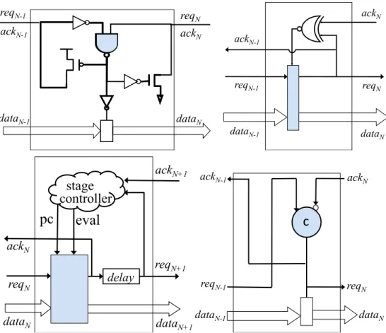
3.7 Synchronization points in various pipeline styles; a) Synchronization point for GasP is anand gate b) Synchronization point for MOUSETRAP _{is a latch; c)} Synchronization point for high capacity is the domino logic; d) Synchroniza-tion point for Sutherland’s Micropipelines is the C element . . . 31

3.8 Abstract model for pipeline stageN with shaded synchronization point . . . 32

(15)

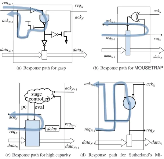
3.10 Revival paths for various pipeline styles . . . 35

3.11 A cycle time composed on one revival and one response time. . . 36

3.12 Indicating revival and response times. . . 36

3.13 A cycle time that crosses two stage boundaries. . . 37

3.14 A cycle that operates simultaneously with the one of Figure 3.13 . . . 37

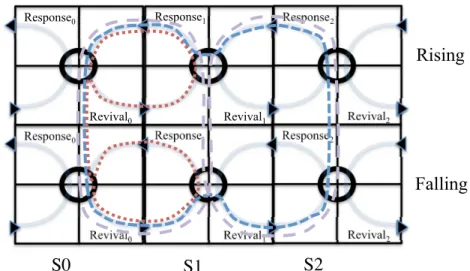
3.15 Stages with asymmetric rising and falling delays require further information for analysis . . . 38

3.16 The process of assigning performance metrics to stages . . . 39

3.17 A hierarchically composable single pipeline stage . . . 41

3.18 A hierarchically composable sequential component . . . 41

3.19 A hierarchically composable parallel component . . . 42

3.20 A hierarchically composable parallel component with speculative conditional 43 3.21 A hierarchically composable non-speculative conditional component . . . 43

3.22 A hierarchically composable data-dependent loop component . . . 44

3.23 Our transformation algorithm . . . 45

3.24 Sample code written in a hierarchical high-level language . . . 45

3.25 Parse tree for code in figure 3.24 . . . 46

3.26 The result of hierarchical composition for the code of Figure 3.24 . . . 47

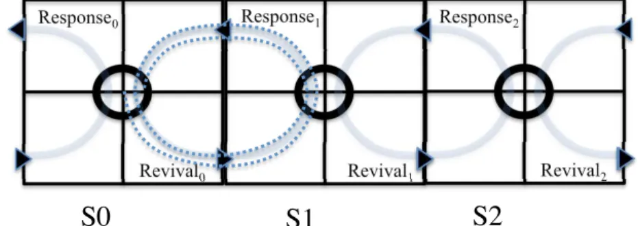
3.27 Snapshots of the operation of a pipeline with steady state behavior. . . 49

3.28 Canopy graphCwith four limiting segments . . . 50

3.29 Parallel composition: a) structure, b) canopy graphs . . . 54

3.30 Canopy graph for a single pipeline stage . . . 54

4.1 A pipelined parallel construct . . . 61

4.2 A parallel construct from CORDIC . . . 62

(16)

4.4 Slack mismatch example . . . 63

4.5 Sequential composition of a parallel construct . . . 65

4.6 Composing in sequence . . . 66

4.7 Canopy graph for sequential composition . . . 66

4.8 A pipelined choice construct . . . 67

4.9 A conditional from CRC . . . 68

4.10 Canopy graph for CRC at p1 = 0.3 . . . 69

4.11 Throughput depends on probability . . . 69

4.12 Canopy graph for CRC at p1 = 0.3 with slack mismatch . . . 70

4.13 Slack mismatch leads to throughput degradation . . . 71

4.14 Clustering decreases throughput . . . 73

4.15 Clustering decreases max throughput . . . 73

4.16 Pipelined GCD loop . . . 75

4.17 Canopy graph analysis for GCD . . . 75

4.18 Our analysis algorithm . . . 76

4.19 Differential equation solver . . . 77

4.20 Abstract syntax tree . . . 78

4.21 Pipelined implementation of Diffeq. . . 78

4.22 Parallel composition ofbranch0 andbranch1 . . . 79

4.23 Canopy graph for loop body . . . 79

4.24 Canopy graph for pipelined loop . . . 80

5.1 Coalescing. . . 87

5.2 Parallelization . . . 88

(17)

5.4 Duplication with Wagging . . . 89

5.5 Buffer Insertion . . . 90

5.6 Slack mismatch in a fork/join construct. . . 92

5.7 Canopy graphs showing slack mismatch . . . 92

5.8 Canopy graphs with slack matching . . . 92

5.9 Key canopy graph intersections . . . 96

5.10 Slack matching algorithm . . . 98

5.11 Sample code for aforloop . . . 99

5.12 A simple implementation of thecomputefunction . . . 99

5.13 A loop pipelined implementation of thecomputefunction . . . 99

5.14 My method of loop flow control. . . 100

5.15 Congestion prevention for pipelined loops. . . 100

5.16 Sample code with feedback . . . 101

5.17 Preventing data hazards in pipelined loops. . . 101

5.18 Pseudocode for generating limiting segment expression . . . 108

5.19 AND-OR tree for the system of Figure 5.22 . . . 108

5.20 Iterative algorithm for bottleneck alleviation . . . 110

5.21 Block level representation of a hierarchical system . . . 111

5.22 A tree representing system of Figure 5.21 . . . 111

5.23 A sample search tree . . . 113

5.24 Exhaustive search with prime solutions as the terminating condition . . . 115

5.25 Code description of exhaustive search . . . 116

5.26 Greedy search evaluates a small number of nodes . . . 116

5.27 Code description of greedy search . . . 117

(18)

5.29 Code description of lookahead search . . . 118

5.30 Recognizing commutative operations to prune the search space . . . 120

5.31 Exploiting commutativity to prune the tree . . . 121

5.32 Pruning search space to avoid identity transforms . . . 122

6.1 Examples of forward timing constraints. . . 145

6.2 a) Beginning state b) Correct end behavior c) Behavior with forward timing violation . . . 147

6.3 Examples of reverse timing constraints . . . 149

6.4 a) Beginning stage b) bubble propagates backwards c) Correct end behavior d) Behavior with reverse timing violation. . . 150

6.5 a) Extra circuitry for forward delay. b) Generic implementation . . . 152

6.6 a) Extra circuitry for reverse delay. b) Generic implementation . . . 155

6.7 ATPG for testing setup time violations. . . 157

6.8 A two-stage pipeline with one level of combinational logic. . . 159

6.9 Timing diagram showing control overrun . . . 159

6.10 A non-linearMOUSETRAP_pipeline _{. . . 164}

7.1 A basicMOUSETRAP_{stage from [55]}_{. . . 168}

7.2 AMOUSETRAP_{fork stage from [55]} _{. . . 168}

7.3 AMOUSETRAP_{join stage from [55]} _{. . . 169}

7.4 A hierarchically composable single pipeline stage . . . 171

7.5 A hierarchically composable sequential component . . . 171

7.6 A hierarchically composable parallel component . . . 172

7.7 A hierarchically composable parallel component with speculative conditional 172 7.8 A hierarchically composable non-speculative conditional component . . . 172

(19)

7.10 Conditional split circuit diagram . . . 175

7.11 Conditional split abstract analysis model . . . 176

7.12 The reverse path for all conditional split circuits . . . 177

7.13 Basic logic minimized expression for conditional split . . . 178

7.14 Generalized C-element implementation of a conditional split . . . 178

7.15 Conditional select circuit diagram . . . 179

7.16 Synchronization point model for the data path of the conditional select . . . . 180

7.17 Synchronization point model for the Boolean path of the conditional select . . 180

7.18 Conditional select optimized for constant Boolean value. . . 181

7.19 Conditional select optimized for forward latency with the assumption that the Boolean value arrives before the data. . . 181

7.20 Data-path setup for a conditional select . . . 182

7.21 Conditional join circuit diagram . . . 183

7.22 Conditional join abstract analysis model . . . 184

7.23 Circuit diagram for merge without arbitration . . . 185

7.24 Merge without arbitration abstract analysis model . . . 186

7.25 Implementation of the data path for a merge . . . 187

7.26 Implementation of the data path for a merge using C-elements . . . 187

7.27 Arbitration stage built around a mutex . . . 189

7.28 Arbiter abstract analysis model . . . 190

7.29 Datapath for arbitration stage . . . 190

8.1 Overall architecture of GCD chip . . . 194

8.2 Basic GCD algorithm before and after simplification of the ring interface. . . 195

(20)

8.4 Area-optimized GCD algorithm, and the dataflow implementation of one

iter-ation . . . 199

8.5 Layout of one iteration . . . 200

8.6 Implementation of a stage: delay matching and control buffering . . . 201

8.7 Detail of the chip interface . . . 203

8.8 Fabricated chip layout and photomicrograph . . . 207

8.9 Testing and evaluation setup . . . 208

8.10 Throughput vs. occupancy for the fastest and slowest chips tested . . . 210

8.11 Estimating the ideal peak internal throughput . . . 211

8.12 Speed increases with increased voltage . . . 212

8.13 Impact of voltage variation on power consumption . . . 213

8.14 Power consumption varies with voltage . . . 214

8.15 Eτ2 _{vs. voltage at maximum throughput} _{. . . 215}

8.16 Impact of temperature on performance . . . 216

8.17 The hierarchical structure of the JPEG example. . . 216

8.18 Performance of the JPEG benchmark before optimizing.. . . 217

8.19 The performance of the JPEG benchmark after loop unrolling . . . 218

8.20 Nodes with detected bottlenecks . . . 219

(21)

Chapter 1 Introduction

1.1 Goals and Solution Strategies

The goal of my work is to support the design of high-performance application specific dataflow

systems (i.e. those that take in a stream of data items and produce a stream of processed

re-sults.) The ability to design such processors quickly and efficiently will likely be important

to sustaining the current level explosive growth of consumer electronics, multimedia

applica-tions, and high-speed networking. My work identifies and addresses several key challenges in

designing these systems.

1.1.1 Challenges to Designing Application Specific Dataflow Systems

One particular challenge is that application specific processors have short design cycles,

be-cause bringing new application specific hardware to market quickly is vital when improved

algorithms and new standards are constantly being created.My work handles this challenge

in several ways. First, it employs the benefits of asynchronous or “clockless” design. The

removal of the clock improves the circuit’s efficiency by eliminating the power requirements

of propagating a global clock signal. Further, the modular nature of asynchronous design can

increase designer productivity and therefore reduce production time and the associated

(22)

system-level optimization for asynchronous dataflow systems. These methods aim to decrease

design times both by improving the speed of the algorithms themselves and by automatically

and systematically completing tasks that designers often spend long hours performing in ad

hoc ways.

Another specific challenge is providing low-level support for the design of high-performance

dataflow systems. Designers want to have some assurance that the systems they create will

operate correctly and be practical to implement at the circuit level. This dissertation presents

new testing approaches that are specific to asynchronous pipelined systems, which can expose

errors caused by manufacturing defects. My work also includes a suite of new circuit-level

designs, which can be connected together modularly to implement a wide variety of system

functionality.

1.1.2 Solution Strategy

In order to make the problem of analyzing and optimizing pipelined asynchronous circuits

more tractable, I focus on a special class of asynchronous systems: those withhierarchically

composed pipelined architectures. Such structures are quite common when the system is

de-signed using high-level translation methods (e.g., Tangram/Haste [45], Balsa [14]) because

high-level specification languages tend to be hierarchically block-structured. Moreover, even

when the design approach is ad-hoc, designers often tend to implement systems with

hier-archical structures. In particular, I target architectures that are hierhier-archical compositions of

sequential, parallel, conditional, and iterative operators. By focusing on this special but

prac-tically useful class of systems, this work is able to leverage information about their hierarchy

to provide fast runtimes while still maintaining accuracy.

1.1.3 Thesis Statement

The problem of analyzing and optimizing pipelined asynchronous systems can be made tractable

(23)

The key insight is that restricting to the hierarchical nature of these systems can be

ex-ploited to make analysis and optimization faster. This dissertation will show that the set of

hierarchical systems is expressive enough to implement a variety of practical systems. The

results will also show that the resulting analysis method is fast and accurate enough to be used

repeatedly in an optimization loop. Finally, the resulting, optimized systems can be practically

realized in hardware.

1.2 Introduction to Asynchronous Design

1.2.1 Definition

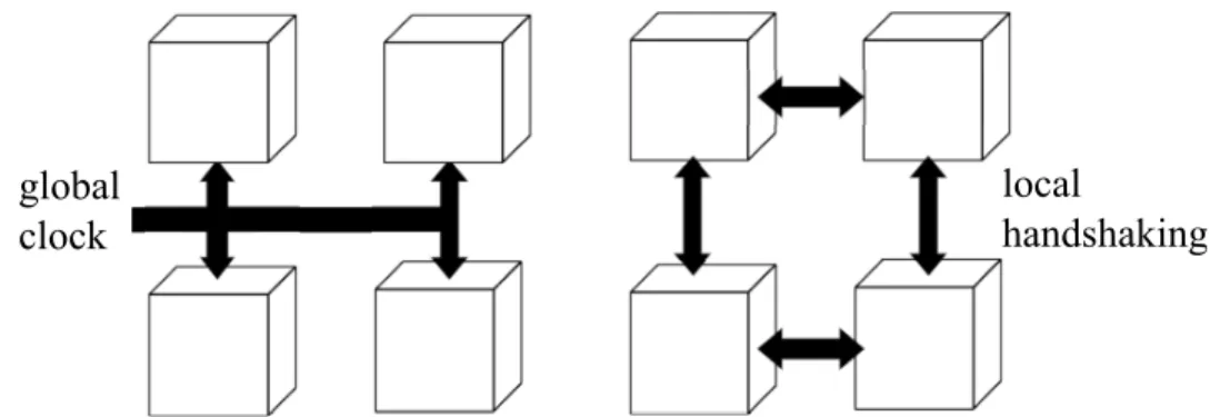
Figure1.1illustrates the fundamental difference between asynchronous design and synchronous

design. While the synchronous system has one global clock that must propagate to the entire

chip, the asynchronous design uses handshakes to synchronize local communications. The

switch from global clocking to local, as-needed synchronization can potentially offer ease

of design due to increased modularity, faster speed because of more concurrency, and lower

energy consumption because switching activity occurs only when and where needed.

global clock

local

handshaking

(24)

1.2.2 Current Uses

As an indicator of asynchronous design’s current commercial success, Handshake Solutions,

a Philips subsidiary, has sold more than 750 million asynchronous microprocessor chips for

use in low-power applications such as cell phones, pagers, smart cards, and cryptochips used

in E.U. passports. In addition, Intel and Sun Microsystems have used asynchronous circuits

in small targeted speed-critical circuits inside their commercial processors.

1.2.3 Future Applications

Asynchronous design will have a significant role in the design of future systems. In future

multi-core systems, on-chip networks that connect hundreds or thousands of heterogeneous

cores will likely be asynchronous in nature, leading to a globally asynchronous locally

syn-chronous (GALS) architecture. Recently, a new style of clocked design has received much

attention from researchers: synchronous elastic design or latency-insensitive synchronous

de-sign. These styles borrow the notion of elasticity (achieved via asynchronous handshaking)

and apply it to clocked design to obtain synchronous elastic systems. Finally, asynchronous

design will likely play a key role in the emerging technologies of nanoelectronic, quantum

and biologically-inspired (e.g., DNA self-assembled) computing, in all of which timing issues

are fundamentally too complex to be addressed by global clocking.

1.3 Past Work and Current Challenges

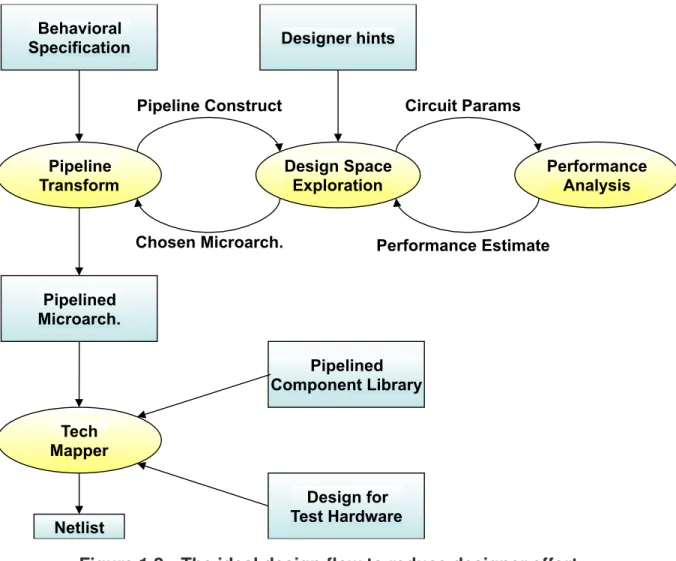
The overall goal of my line of research is to create a fully automated toolflow for the design

of high-throughput asynchronous circuits that begins at a designer specification and ends with

a gate-level hardware specification. Figure 1.2 shows an example design flow, which gives

context for the work presented in this dissertation. If fully automated, this design flow will

achieve the goals of creating efficient, high-performance circuits with low designer-time cost.

(25)

the overall goals, describe the current work that has been done in each area, and outline the

remaining work that this dissertation will add to the design flow.

Pipeline Transform Behavioral Specification

Performance Analysis Design Space

Exploration Designer hints

Pipelined Microarch.

Pipelined Component Library

Netlist

Design for Test Hardware Pipeline Construct

Chosen Microarch. _{Performance Estimate} Circuit Params

Tech Mapper

Figure 1.2: The ideal design flow to reduce designer effort.

1.3.1 High-level Code to Low-level Designs

In the design flow of Figure1.2, the designer first gives a high-level behavioral specification

for the circuit. Next, that control-driven specification is turned into a data-driven pipelined

architecture. My work does not focus on this transformation step, because much current and

ongoing work done by others has effectively targeted this area. Specifically, Hansen [19] has

(26)

specification. Work done by Budiu [8] used C as the input language to create a hardware

specification in which data flows directly from producer to consumer. Kapasi takes a different

approach to specifying data flow hardware by introducing new language constructs that are

tailored to data flow design [24]. Though Chapter3of this dissertation does give one possible

algorithm for converting a specification written in a high-level language to a pipelined system,

this is offered only for completeness and does not limit the work of this dissertation to using

only that one approach for the first pipeline transform step of the design flow.

1.3.2 Design-space Exploration

Automated design-space exploration is key to reducing designer effort. In the design flow of

Figure1.2, design space exploration takes a non-optimized pipelined circuit as an input and

re-turns an optimized version of the circuit. Since my work targets high-throughput systems, the

final circuit should be optimized to meet some throughput goal, possibly with additional

con-straints on other cost functions such as delay or energy. The design space exploration should

ideally take place with little to no direct intervention on the part of the designer. Currently,

many circuit designers use time consuming ad hoc techniques based on designer knowledge

and experience. More systematic approaches presented by Beerelet al.[3], Prakashet al.[47],

and Smirnovet al.[1] remove bottlenecks by strategically adding buffer stages to the circuit.

Other approaches target latency rather than throughput. One such approach is the CASH

com-piler by Budiu and Goldstein [8], which translates an ANSI C program into data-flow

hard-ware. A different approach by Theobald and Nowick [63] targets generation of distributed

asynchronous control from control-dataflow graphs, with the objective of optimizing

commu-nication between the controllers, and between a controller and its associated datapath object.

To my knowledge, a system-level design space exploration system that focuses on throughput

does not currently exist. My work on constrained optimization for pipelined systems aims to

(27)

1.3.3 Performance Analysis

Performance analysis is an integral part of design space exploration, because optimization

often requires repeated analysis to monitor the effects of changes to the circuit. As seen in

Figure1.2, the design space exploration method uses performance analysis repeatedly, which

indicates that fast and accurate performance analysis is important to making the design

ex-ploration work. Several innovations in the area of performance analysis of pipelined circuits

serve as the basis of the work of this thesis. The idea that the throughput depends on the

occu-pancy of a pipeline, which is the foundation of much of the analysis-level work of this thesis,

was first introduced in a doctoral thesis by Williams [67] and later expanded upon by

Green-street [18] and Lines [31], though none of these works provided a system-level approach.

In addition, more general analysis methods [29][71] [36] can estimate the performance of

entire systems, proving that accurate system-level throughput estimates can be obtained for

pipelined asynchronous systems. Brining these ideas together, my analysis work provides a

fast analytic solution like that of Williams [67] while maintaining some of the versatility found

in past system-level analysis methods.

1.3.4 Circuit Components

The design space exploration step produces an optimized pipelined microarchitecture. To be

realized in practice, every component within the microarchitecture must be implemented by a

corresponding circuit component. Many pipeline circuit styles have already been developed,

which serve as the basis for implementing any high-throughput pipelined system.[61, 15,

42, 59, 55, 72] Micropipeline styles that achieve high-speed while maintaining low control

overheads enable the construction of fast and efficient asynchronous pipelines. My work in

this area adds on toMOUSETRAP_{, a high-speed, low-overhead pipeline implementation [55].} Existing MOUSETRAP_{circuits can be used to implement a variety of structures, but are not} expressive enough to implement all the possible behavior in the set of circuits that the design

(28)

can, together with existing circuits, implement common hierarchical structures. These circuits

can be composed together modularly to form a wide variety of structures and behaviors.

1.3.5 Testability

Finally, the design flow incorporates the design for testability. Incorporating testing into a

design flow is vital to the success of any design flow, because designers are hesitant to use

a technology that cannot be tested. Luckily, much work has already been done in the area

of testing for asynchronous pipelines. Pagey et al. [43] proposed methods for generating

test patterns to test stuck-at faults in traditional micropipelines. Another approach that was

adapted for use with micropipelines is by [27], which focuses on test sequence generation for

testing both stuck-at and delay faults insideC-elements—circuits that are often used as local

synchronizing elements in asynchronous systems. My work on testing is based most closely

on the work of Shiet al.[53], which is specifically targeted to testing high-speed asynchronous

pipelines. My testing work focuses on achieving high fault coverage while trying to keep the

design-for-test overheads low.

1.4 Contributions

The work of this thesis focuses on one type of asynchronous circuits—high-throughput

steam-ing systems that are hierarchical in nature—in order to provide a great depth of resources for

designing these types of circuits. Contributions range from high-level abstractions for circuit

modeling to low-level circuits that are used as the basis for circuit design.

1.4.1 Modeling and Abstractions

Chapter3 presents the models and abstractions that are used throughout the rest of the

(29)

system, defines the structure of a hierarchical system, and formalizes use of canopy graphs for

performance analysis.

1.4.2 Performance analysis

Chapter 4 addresses the problem of system-level performance estimation. Although

deter-mining the performance of an arbitrary asynchronous system is NP-hard, my solution focuses

instead on analyzing a special subclass: systems that are hierarchically composed of basic

pipeline stages using sequential, parallel, iterative, and conditional operators. This restricted

class is actually still quite rich, and includes most commonly used system topologies. By

ex-ploiting hierarchy, my algorithm achieves an expected linear running time. Results show that

non-trivial examples with over 100 stages can be analyzed in less than 10 milliseconds.

1.4.3 System-Level Optimization

Chapter5presents optimization methods that leverage the fast analysis method presented in

Chapter4. Identification and elimination of bottlenecks is an important part of any design flow

that aims to produce high-throughput systems. This thesis includes (i) a bottleneck detection

algorithm that leverages performance analysis to pinpoint the parts of an asynchronous

sys-tem that limit throughput, and (ii) a bottleneck alleviation algorithm that reports all potential

bottlenecks to the designer and suggests modifications. A specific challenge is to overcome

the performance bottleneck due to algorithmic loops. I have introduced a systematic approach

for improving the throughput of algorithmic loops by allowing multiple problem instances to

be computed concurrently within a single loop hardware (i.e., multi-token loops).

1.4.4 Testing and Design for Testability

Chapter6presents a testing approach to uncover timing violations within asynchronous pipelines.

(30)

approach targets a subclass of much interest to asynchronous designers: relative timing

con-straint violations. In particular, certain asynchronous circuits achieve high performance by

making local timing assumptions. I have introduced the first practical method for testing

for violations of these relative timing assumptions in pipelined systems. The approach is

minimally-intrusive and includes both test application and test vector generation.

1.4.5 Circuit-Level Design

Chapter7presents the low-level pipeline stages that form the basis for implementing pipelined

asynchronous systems. My component library includes circuit-level designs of all commonly

used building blocks (i.e., design primitives), including pipeline stages, forks/joins,

condition-als and loops, arbitration stages, etc. These designs were carefully constructed so as to obtain

high throughput and low latency.

1.4.6 Case Studies

To demonstrate and evaluate these circuits, Chapter8presents asynchronous case study chip

that implements Euclids iterative GCD algorithm; it was fabricated at IBM foundry in a 130nm

CMOS process. The chip is one of only a few high-speed asynchronous chips that have been

demonstrated so far, achieving the equivalent of 1 GHz operation, and robustness to wide

variations in supply voltage (0.5-4V) and temperature (-45-150C), and has helped validate my

design and test approaches. In addition, the chapter uses the analysis and optimization of a

JPEG encoder as a detailed example of the steps taken to produce a final, optimized circuit.

The results show a 40x improvement for this example.2

1.5 Dissertation Organization

The remainder of this document is organized as follows. First, Chapter2 gives background

(31)

Next, Chapter 3describes the abstractions and models that will be used throughout this

dis-sertation. It also introduces new notations and definitions relevant to asynchronous design that

are extensions upon previous work.

Chapter 4 introduces my analysis method. It first presents the analysis of the four

hi-erarchical components considered in this dissertation—sequential, parallel, conditional, and

iteration—and then describes how to bring them together to form a system-level,

hierarchi-cal analysis method. Chapter5 goes on to present an optimization method that builds off of

the analysis. It first describes a set of transformations that can potentially improve

perfor-mance, then gives a method for detecting the location of bottlenecks within a system, and

finally defines a framework for iteratively applying optimizing transformations to remove all

the bottlenecks of a system.

Chapter 6 describes a testing method that applies to pipelined asynchronous systems.

Chapter7 provides low-level support for design by specifying a suite of five circuits that—

together with circuits from past work—can be used to implement a wide variety of

asyn-chronous systems. This chapter can serve as a reference for those who wish to implement any

of the hierarchical structures described in this dissertation. Finally, Chapter8gives two case

studies in asynchronous design. The first one, a system that calculates the greatest common

di-visor of two numbers, was fabricated in silicon and tested extensively. It serves as an example

(32)

Chapter 2 Background on Asynchronous Design

2.1 Asynchronous Pipelines

In a pipelined asynchronous system, parts of the circuit synchronize locally using a

request-acknowledge handshake protocol. These handshakes control the flow of data into and out

of registers, which are usually implemented as latches. A pipeline operates correctly if the

handshaking protocol prevents data from being lost or overwritten while still allowing for the

flow of data between stages.

Figure2.1shows the basic structure of a self-timed pipeline. Each pipeline stage consists

of a controller, a storage element (“data latch”), and processing logic. Typically, a stage

generates a requestto initiate a handshake with its successor stage, indicating that new data

is ready. If the successor stage is empty it accepts the data and performs two further actions:

(i) it acknowledges its predecessor for the data received and, (ii) initiates a similar handshake

with its own successor stage. Many variations on this basic protocol have been developed, and

a variety of asynchronous pipeline controller implementations exist.

2.1.1 Data Encodings within Asynchronous Pipelines

Pipeline styles can also be categorized based on the data encoding employed. Using data

(33)

Figure 2.1: A simple self-timed pipeline

[38,34], so this section will not provide a full description of possible data encodings. Instead,

it will give some idea of the main types of data encodings used.

Bundled Data

A simple yet effective approach is the bundled data encoding, which is also known as

single-rail. Each data bit is represented by exactly one wire, with one additional wire for the request

bit. While the data bits are processed by a block of logic within the stage, the request bit

must go through some matched delay—a set of gates that slows the outgoing request so it

stays coherent in time with the data. This style is simple and practical, but it does not take

advantage of function blocks that have variable delays.

Dual-Rail Encoding

Dual-rail data encoding uses two wires per data bit, so that the request signal is essentially

built in to the encoding. Table 2.1 shows one possible dual-rail representation that encodes

both the value of the data and the presence of new data.

This encoding scheme allows the stage to indicate completion as soon as it is finished,

(34)

Table 2.1: Dual rail data encoding. Dual-rail code

0 0 data not ready

0 1 0 request

1 0 1 request

1 1 unused

2.1.2 Asynchronous Handshaking Protocols

two-phase Protocols

Two phase protocols have handshaking cycles that are made up of two events. Specifically,

the value of the request changes once and then the value of the acknowledge changes once

to complete the handshake. As a result, 2-phase protocols use transition based encodings: a

transition on a line rather than the value of the line indicates an event.

four-phase Protocols

Four phase protocols have handshaking cycles that are made up for four events. Typically,

the request goes high and the acknowledge goes high as a response. Then the request goes

low to a reset value, and the acknowledge also resets to a low value. This protocol has more

events than a two-phase protocol, but the logic implementations are often simpler, because

level-based logic is a simpler design style than transition-based logic.

2.1.3 Asynchronous Pipeline Styles

Many different implementations for asynchronous pipelines have been developed, which use

different combinations of data encodings and handshaking protocols. [61, 15, 42, 59, 55,

72, 67] In this dissertation, I use the following four circuit styles as examples whenever the

(35)

!"

req

_N

ack

_N

ack

_N-1

req

_N-1

data

_N-1

data

_N

Figure 2.2: Sutherland’s Micropipeline with Muller C-element.

Sutherland’s Micropipelines

Suterland’s Micropipeline style [61] is a two-phase controller that uses bundled data. As

shown in Figure2.2, it uses the Muller C-element [40] as the control circuit. Since the output

of the C-element to the latch uses transition signaling, the latch is a special transition sensitive

latch. When the pipeline line is in operation, every transition on the request wire—either high

to low or low to high—indicates that a new data is available. The next stage will send back a

corresponding acknowledge signal when it has finished processing the previous data.

MOUSETRAP Pipelines

MOUSETRAP _{[55], shown in Figure}_{2.3, is a two-phase pipeline style that uses static logic.} Since MOUSETRAP_{uses transition signaling for the requests and acknowledges, every} tran-sition on a request wire indicates new data is ready and every trantran-sition on an acknowledge

wire indicates that old data can be overwritten. Thus, when the request and acknowledge

go-ing into a stage are the same, the stage becomes “empty” and when they are different the stage

becomes “full”. The latches that hold data begin transparent and become opaque just after

(36)

req

_N

ack

_N

ack

_N-1

req

_N-1

data

_N-1

_data

N

Figure 2.3: TheMOUSETRAPpipeline style.

as a transition to level converter.

GasP Pipelines

GasP _{[59] is a four-phase pipeline style that uses static logic. The data latches in a} GasP

pipeline begin closed, and must open and then close again upon receiving each new data item.

The most distinctive feature ofGasP_{is that a single wire, called the state conductor, is used}

to transmitboththe request and acknowledge signals between a pair of adjacent stages. A low

signal on the state conductor wire indicates that the previous stage is“full” and a high signal

indicates that it is “empty”.

The controller for GasP_{is a self resetting}_NAND_{, as shown in Figure} _{2.4. When both of}

the inputs to theNANDgo high, it goes low. After some delay, this low transition triggers the

NANDto reset back to high. Specifically, two possible reset paths, r1 andr2, can cause the NANDto go high again. Pathr1consists of one pull up transistor and one inverter (inva). Path

(37)

req_N-1

req_N

ack_N ack_N-1

data_N-1 data_N

Figure 2.4: The GasP pipeline style.

High-Capacity Pipelines

The high-capacity (HC_{) pipeline [54] is a four-phase pipeline style that uses dynamic logic.}

It islatchless. Instead, the dynamic logic of each stage has an “isolate phase”, in which its

output is protected from further input changes. Specifically, during the isolate phase, the logic

is neither precharging nor evaluating.

AnHC_{pipeline stage simply cycles through three phases. After it completes its evaluate}

phase, it enters its isolate phase and subsequently its precharge phase. As soon as precharge

is complete, it re-enters the evaluate phase again, completing the cycle.

2.2 Performance Analysis for Asynchronous Pipelines

2.2.1 Performance Metrics for Pipeline Stages

There are three metrics typically used to characterize the performance of a self-timed pipeline:

forward latency, reverse latency, and cycle time. The forward latency is simply the time it

(38)

delay

pc

_eval

ack

_N

req

_N

req

_N+1

ack

_N+1

data

_N

_data

_N+1

stage

controller

Figure 2.5: The high capacity pipeline style.

isFi, then the latency of the entire pipeline is:

LPipeline = X

i

Fi (2.1)

Similarly, the reverse latency characterizes the speed at which empty stages or “holes” flow

backward through an initially full pipeline. The reverse latency of the entire pipeline is simply

the sum of the stage reverse latencies:

RPipeline = X

i

Ri (2.2)

The cycle time of a stage, denoted byTi, is the minimum time that must elapse after a data item

is produced by that stage before the next data item will be generated. Since a complete cycle

of a stage typically consists of transmitting a data item forward followed by propagating a

hole in the reverse direction, the following relationship holds for most handshaking protocols:

(39)

The maximum throughput a stage can support is simply the reciprocal of its cycle time. The

cycle time of a linear pipeline is limited by the cycle time of its slowest stage:

tptPipeline = 1.max

i (Ti) (2.4)

2.2.2 Canopy Graph Analysis

The classic work on performance analysis of asynchronous pipelines by Williams and Horowitz

[67] introduces the “canopy graph” to characterize the performance of a pipelined ring. Our

approach builds upon this to handle more general systems.

Ring Performance Analysis

One useful metric of ring performance is the number of times any data item crosses a

par-ticular stage in the ring per second; we will refer to this measure as thering frequency. The

performance of the ring is highly dependent on itsoccupancy, i.e.,the number of data items

revolving inside it. When the number of data items is small, the ring frequency is low, and

the pipeline is said to be “data limited.” On the other hand, when nearly every stage of the

pipeline is filled with data items, the performance is once again limited, because holes are

needed to allow data items to flow through the pipeline. In this scenario, the pipeline is said

to be congested, or “hole limited.”

Data Limited Operation. If there arek data items in the ring, then in the time a

particu-lar data item completes one revolution around the ring (i.e., P

iFi), all k items would have

crossed each ring stage. Therefore, the maximum ring frequency attainable is proportional to

the ring occupancy:

Ring Frequency _≤ k.X

i

Fi (2.5)

(40)

1 2 N-2 N-1 0 Data limited region Hole limited region

Max ideal throughput

= 1/(L+R)

Limited by a slow stage

Slope =1/

Σ

L Slop

e = 1/

_Σ

R

Ring Occupancy, k

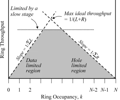
Ri ng T hr ou gh pu t N

Figure 2.6: The upper bounds on the maximum ring frequency: shaded area represents operating region

ring frequency is limited by the number of holes in the ring. If there areh holes in the ring,

then in the time a particular hole completes one revolution around the ring (i.e., P

iRi), all

h holes would have crossed the each stage, 0 in a direction opposite to data. Thus, if N is

the number of stages in the ring, then h = N ₋k, and we have the following bound on the performance:

Ring Frequency _≤ (N ₋k).X

i

Ri (2.6)

Figure 2.6 shows a plot of the ring frequency versus its occupancy. The rising portion

of the graph represents the data limited region, where performance rises linearly with the

number of data items. The falling portion, similarly, represents the hole limited region, where

performance drops linearly with a decrease in the number of holes.

Limitations Due to a Slow Stage. If all the stages in the ring have similar forward and

reverse latencies, then the maximum attainable performance will be the frequency at which

(41)

is the inverse of the cycle time of each ring stage: 1/T = 1/(L+R). However, if some

stages are slower than others, then the ring frequency will be limited by the cycle time of the

slowest stage. In the figure, the horizontal line represents the maximum operating rate that

can be sustained by the slowest stage in the ring [67]:

Ring Frequency _≤ 1.max

i (Ti) (2.7)

The overall ring performance will always be constrained to lie under the canopy formed by

the three lines in Figure2.6.

Linear Pipelines

The behavior of a linear pipeline,under steady-state operation,can be modeled as that of a

self-timed ring. In particular, in steady state, as one item leaves the right end of the pipeline,

another item enters on the left. As shown by Lines [31] and Singh et al. [57], the linear

pipeline’s throughput is correctly modeled as a canopy graph, with the same three constraints

on its operation (data limited, hole limited, and constrained by local cycle times).

However, there are two key differences that must be noted. First, the occupancy in a linear

pipeline can be fractional. That is, unlike a ring which always contains an integral number of

items, a linear pipeline can have anaverage occupancy that is non-integral (e.g., 4.5 items)

because of phase differences between entering and exiting items.

Second, a linear pipeline can actually operate in the entire region under the canopy. In

contrast, the operating point of a ring in steady state is typically on the boundary of the canopy.

The reason for this difference is that the ring analysis assumed that the ring is isolated and

operates autonomously without any interaction with the environment; therefore, it operates at

the maximum throughput possible for a given occupancy. On the other hand, a linear pipeline’s

operation is constrained by both the left and right environments, which can force it to operate

(42)

!" #" $%&'()*+" ,--./0)-1" #" a) b)! !" 2 3 4% . 5 3 / . 6"

Figure 2.7: Parallel composition: a) structure, b) canopy graphs

!" #" $%&'()*+"

!" #"

a)!

b)! ,--./0)-1"

2 3 4% . 5 3 / . 6"

Figure 2.8: Sequential composition: a) structure, b) canopy graphs

Parallel and Sequential Composition

As shown by Lines [31], canopy graph analysis can also be applied to parallel and sequential

compositions of linear pipelines.

For the fork-join parallel structure of Fig.2.7a, the throughput of the composition is

con-strained by the intersection of the canopy graphs of the branches. The reason is that the

operation of the fork-join pair is constrained so that (i) the throughput of each branch is the

same, and (ii) the number of tokens in each branch is the same (assuming they were initialized

empty). The result of the intersection of the constituent canopy graphs is also a canopy graph

as shown in Fig.2.7b.

Similarly, when two pipelines are composed sequentially, as in Fig. 2.8a, the throughput

of the composition is constrained by the horizontal sum of the canopy graphs of the two

(43)

but the total occupancy is now the sum of the occupancies of the two pipelines. That is, the

composition can attain any throughput that both of the pipelines can sustain, and for each such

throughput, the net occupancy is simply the sum of the two occupancies. The result is also a

(44)

Chapter 3 Models and Abstractions

Throughout the thesis, most of the discussions and proofs will deal not with the complex,

underlying circuits but with the more abstract models. This chapter defines the models that

will be used throughout this thesis and defines how they relate to real systems. First Section

3.2 gives the models for the performance of an individual stage and presents a method for

mapping from a pipelined circuit to the abstract representation used in later chapters. Section

3.3fully defines the set of hierarchical circuits that this thesis analyzes, and gives an example

of the steps from high-level code to a pipelined representation. Finally3.4defines and further

described the use of the canopy graph for modeling system-level performance information.

3.1 Background

3.1.1 Performance Metrics for Pipeline Stages

Three performance metrics are typically used to describe the performance of pipeline stages:

forward latency, reverse latency, and cycle time. Following are the classical descriptions of

(45)

Forward Latency

The forward delay, also denoted as LF, is the difference between the time that a request is

received by an empty stage and the time that a request is received by the following stage.

Figure3.1illustrates the forward delay of one stage.

!"#$%&

!"#'()

*+,'()&

*+,$%&

Figure 3.1: Forward delay for a pipeline stage

Reverse Latency

The reverse delay, also denoted asLR, is the difference between the time that an acknowledge

is received by a full stage and the time that an acknowledge is received by the previous stage.

It is also often useful to think of the reverse delay as the time for one “hole” to travel in the

reverse direction of the flow of data. Figure3.2illustrates the forward delay of one stage.

!"#$%&

!"#'()

*+,'()&

*+,$%&

Figure 3.2: Reverse delay for a pipeline stage

Cycle Time

Cycle time, orT, is the time for a stage to progress from some state in relation to a data item

until the time it arrives at the same state with the subsequent data item. Figure3.3 shows a

representation of the cycle time. Note that cycle time can cross stage boundaries, and that it

does not necessarily include the entirety of either the forward or reverse cycle time for the

(46)

!"#$%&

'()*+,&

!"#*+,

'()$%&

Figure 3.3: Cycle time for a pipeline stage

3.1.2 Abstractions for Asynchronous Pipelined Systems

One common representation for an asynchronous circuit is the Petri net, which has been used

in much past work [30][36][71]. Petri nets are capable of capturing the high concurrency

inherent to asynchronous systems. Moreover, timed petri nets, which assign a delay to every

event within the system, allow for thorough analysis of the timing of the asynchronous system.

[36].

The power of using a petri net model lies in its ability to represent all possible

connec-tions and configuraconnec-tions of a general asynchronous system. This kind of low-level modeling

of connections is necessary when analyzing systems with complex connections and

irregu-lar topologies. The work in this thesis, however, focuses on systems that are composed of

repeated instances of pipeline stages that are further organized hierarchically. For these

pur-poses, a timed petri net representation is not necessary; the essence of the system can be

captured by a more abstract, high-level representation.

3.1.3 System-level Performance Models

The most straightforward method for describing the performance of a pipelined system is to

give one number: the throughput. Variations on the single-number performance

characteriza-tion include reporting the cycle time, bounding the time separacharacteriza-tion of events, or finding the

global critical cycle time for the system [36][30][70][65]. Each of these metrics provides a

one-dimensional view of the performance of a circuit, in that a single performance number for

(47)

Williams and Horowitz [67] first introduced the use of a second dimension, occupancy,

to characterize the performance of a system. Here, occupancy is defined to mean the total

number of distinct data items that are contained in the entire pipelined system. This thesis

relies heavily on the throughput vs. occupancy graph, also known as the canopy graph, first

introduced for analyzing the performance of a pipeline ring. Later, Lines [31] and Singhet

al.[57] applied this model to sequential pipelines, and Lines [31] further used it for systems

consisting of a parallel operator. More details on the derivation and methods of this work can

be found in the background section2.2.2of this thesis.

3.2 Modeling Asynchronous Pipeline Stages

As described in Section 2.1.3, many different types of asynchronous pipelines exist. My

method for analyzing pipelines, however, is independent of the particular pipeline style used.

This section describes how to map an actual asynchronous pipelined stage onto a

representa-tion that is independent of implementarepresenta-tion by abstracting away the unnecessary details while

retaining the necessary performance information.

3.2.1 Delay Models

The analysis method described in this thesis uses a fixed delay model. The commonly used

bundled data encoding, which was described in Section 2.1.3, is very accurately modeled

using fixed delays. Other data encodings, such as dual-rail, can have data-dependent execution

times for individual stages. Though this work does not directly address probabilistic delays,

it can still be used to perform worst case analysis by setting the fixed delays to be equal to the

worst case delay for each stage. Worst case analysis is a useful lower bound on performance.

(48)

3.2.2 Performance Metrics for System-Level Analysis

Figure 3.4 shows the abstract model for an asynchronous pipeline stage that will be used

throughout the rest of this thesis. Each stage is represented by a box. This is a further

abstrac-tion of the pipeline stage shown in Figure2.1, which removes the unnecessary details of the

stage’s controller, latch, and logic.

The connections between stages are represented by arrows. The direction of the arrows

indicates the direction of the flow of data while the flow of “holes” is implied to be in the

op-posite direction. The internal workings and even the handshaking signals have been removed

for simplicity and are indeed not necessary to perform analysis on this system.

!"#$!%#&!

!'#(!)#&!

!"#$!%#&!

!'#(!)#&!

!"#$!%#&!

!'#(!)#&!

!"#$!%#&!

!'#(!)#&!

!"#$!%#&!

!'#(!)#&!

!"#$!%#&!

!'#(!)#&!

!"#$!%#&!

!'#(!)#&! !"#$!%#&!

!'#(!)#&!

!"#$!%#&!

!'#(!)#&! "#$!%#&!

'#(!)#&!

Figure 3.4: General model for a pipelined system.

Each stage is also annotated with the local performance metrics that are necessary for

performing analysis: forward latency, reverse latency, cycle time, and capacity. These four

metrics fully characterize the performance of each individual stage for the purposes of

per-forming system-level analysis. This notation for graphically describing a pipelined system

will be used throughout this thesis. For conciseness, the graphical representations often omit

the cycle time and capacity, as has been done in Figure 3.5. If not specified, cycle time is

assumed to be the sum of the forward and reverse latencies and the capacity is one.

This thesis uses the same definition of cycle time as give in background section 3.1.1.

However, the definitions of forward and reverse latency are slightly changed, capacity is a

(49)

!"#$

#"#$

!"%$

#&"#$

!"#$

#"#$

!"#$

#&"#$

Figure 3.5: Model for a pipelined system used throughout this thesis.

Capacity

The capacity of a single stage to hold data is a feature of the chosen pipeline style. All

commonly used pipeline styles have a capacity of either one or one half data items per stage,

although other capacities are possible in theory. A capacity of one indicates that two stages

in a row can both contain distinct data items while a capacity of one half indicates that every

other stage can contain a distinct data item.

3.2.3 Determining Performance Metrics

Although the models used for analysis do not depend on the type of pipeline stage being used,

determining the values of the four parameters for each stage–which must take place before

analysis–does depend on the type of pipeline stage being used. In particular, one cannot

always assume that cycle time for a stage be calculated using the forward and reverse delays

only.

This section describes my technique for determining the necessary metrics. The remainder

of the thesis assumes that these metrics have already been determined, and the accuracy of the

performance analysis will, of course, depend on the accuracy of performance metric values

(50)

Challenges to Determining the Performance of a Single Stage

A common method for finding the cycle time is simply summing the forward and reverse

cycle times [67, 58]. Though this method is it simple and elegant, it does not always give an

accurate local cycle time. The local cycle time often includes the delays of gates across two or

more pipeline stages, so summing the forward and reverse latencies is inaccurate when gates

in adjacent stages have differing delays.

As an example, see cycle time for the pipeline stageS0shown in Figure3.6. Compare the

sum of the forward and reverse latencies of the stage to the cycle time.

LF0+LR0 =dL0+dxnor0+dL0

T0 =dL0+dL1+dxnor0

Note that the expressions are identical only if the delays of latchesL0andL1are the same.

Therefore, ifdL1is greater thandL0, then the sum of the forward and reverse delays will be an underestimate of the actual cycle time forS0.

L0 L1

xnor0 xnor1

Figure 3.6: Cycles cross stage boundaries.

Synchronization Point Method for Determining Performance Metrics

Despite this subtle difficulty in assigning performance metrics to individual stages, it is still

possible to assign local cycle times to individual stages. In particular, if the properties of

neighboring stages are known at the time of analysis, the difference in gate delays can be

taken into account when assigning performance metrics to every stage. If the connections

Analysis and optimization for pipelined asynchronous systems