Vol. 47 - No. 1 - Spring 2015, pp. 33- 40 )AIJ-MISC)
٭
Corresponding Author, Email: [email protected]
Peaking Attenuation in High-Gain Observers Using
Adaptive Saturation: Application to a Ball and Wheel
System
S. D. Yazdi Mirmokhalesouni
1and M. J. Yazdanpanah
2*
1- Advanced Control Systems Lab, Control and Intelligent Processing Center of Excellence (CIPCE) at School of Electrical and 2- Computer Engineering, College of Engineering, University of Tehran, Tehran, Iran.
ABSTRACT
Despite providing robustness, high-gain observers impose a peaking phenomenon, which may cause
instability, on the system states. In this paper, an adaptive saturation is proposed to attenuate the undesirable
mentioned phenomenon in high-gain observers. A real-valued and differentiable sigmoid function is
considered as the saturating element whose parameters (height and slope) are adaptively tuned. The
corresponding feedback and adaptation laws are derived based on the Lyapunov and LaSalle theorems to
guarantee the asymptotic stability property for the closed-loop system’s equilibrium point. Compared to the
conventional high-gain observers which suffer from states’ peaking, it is possible to increase the observer’s
gain, up to a higher level, under which not only all system states and the adaptive saturation elements remain
stable, but also robustness is reinforced in the presence of uncertainties and/or non-similarities in the system
and observer’s dynamics, respectively. Both theoretical analysis and simulation results confirm the efficiency
of the proposed scheme.
KEYWORDS
1. INTRODUCTION
Over the last decades, a variety of laboratory experimental setup such as ball and beam and inverted pendulum, have been built for some researches in nonlinear systems. These systems have attracted researchers’ attention because of their inherent nonlinearity, open loop instability, under-actuation, etc. Therefore, many works have been done on such systems. In this article, a ball and wheel system is considered, whose schematic overview is depicted in Figure 1. For the purpose of controlling the mentioned system, authors of [1] measured angular positions by designing sensors. But, the angular velocities were measured from the angular displacement traveled per unit time. In this article, an output feedback is used to prevent such measurements.
In the ground of some control systems, measuring all state variables are neither affordable nor possible. In this article, output feedback is applied to estimate state variables using a high-gain observer. There are two advantages in this regard. First, there is no need to measure all state variables. Second, a high-gain observer makes it possible to consider unmodeled dynamics because of its robustness. The theory of high-gain observers has been developed over two last decades. It was used for designing robust observers in linear systems [2]. Earlier works in high-gain observer design for nonlinear systems started in the late 1980s [3]. High-gain observers are also developed to estimate system states containing time delay [4]. The authors of [5] developed a high-gain observer structure in the presence of sampled output measurement. Finite time observation method is proposed in [6].
Khalil et al. have considered a situation where due to absence of Lipchitz condition, the observer gain may become too large resulting in the instability of closed-loop system. This instability is explained by peaking phenomenon which means that a sufficiently large gain causes impulsive behavior in the response. The effect of peaking phenomenon on instability is also considered by Sussmann and Kokotovic [7] in high-gain state feedback. In the meantime, this phenomenon had been considered in the linear systems in [8]; however, the effect of peaking on
nonlinear systems was studied in [9] for the first time, where it was suggested that the designed controller should be a globally bounded function of the estimated variables to be saturated during the peaking period. The work by Esfandiari and Khalil [9] brought attention to the peaking phenomenon as an important feature of high-gain
observers. It showed that the interaction of peaking with nonlinearities could induce finite scape time. In particular, in the lack of global Lipschitz conditions, high-gain observers could destabilize the closed-loop system as the observer gain is driven sufficiently high. Since, the dynamics of high-gain observer are much faster than those of the closed loop dynamics; the peaking period is very short compared with the simulation period. This separation of time scales is used in [9] to prove stability of the closed-loop system with output feedback controller. Shortly after publishing [9], Teer et al. used its ideas to prove the first nonlinear separation principle and develop a set of tools for semiglobal stabilization of nonlinear systems [14]. In [10], a nonlinear gain is used for having a suitable trade-off between higher observer gain in transient period to increase convergence rate and decrease the effects of uncertainties and/or non-similarities on error.
In this article, an adaptive structure is proposed for saturating the control signal, which not only attenuates peaking phenomenon to make the closed-loop system unstable but also results in a better performance in the sense of energy of the error between the actual states and their estimations. Moreover, since the system’s dynamical model is adopted from [1] in which no disturbance is assumed, to examine the proposed method in the presence of uncertainties, the observer’s dynamics are simplified, as further elaborated, to show robustness feature of the proposed high-gain observer. In fact, some parts of dynamics are overlooked in the observer’s structure though they should contribute in the response. Despite simplifying dynamics, deliberate elimination of some parts of observer’s dynamics is successfully compensated due to robustness provided by high-gain property.
The rest of this paper is organized as follows. In Section 2, the model of the system and its parameters are presented. In the first part of Section 3, a control law is given using the feedback linearization technique. The structure of the high-gain observer is presented in the second part of Section 3. The last part of Section 3 is dedicated to designing an adaptive saturation structure for controlling signal restriction in order to prevent peaking phenomenon. Then, it is shown that the proposed method results in an asymptotically stable closed-loop system. In Section 4, the simulation results concerning cases with adaptive and non-adaptive saturation elements are presented. Finally the conclusion is made in Section 5.
2. MODEL DESCRIPTION
illustrates the basic features of the system. There are some assumptions for this model. First, the coefficient friction is large enough for the ball to just roll on the wheel with no slip. Second, the ball is always in contact with the wheel. The mentioned model reads below:
(x) g(x) u
x f
(1)
where 2 4 1 4 4 1 0 sin
(x) , (x)
0 sin
x
ax b x c
f g
x
px q x r
(2)
And the parameters a, b, c, p, q and r are defined below:
2
2 2
(7 I 2 r m )(r r )
w m
a w w b b w
r K a R 2 2
(5 I 2 m )
(7 I 2 r m )(r r )
w w b
w w b b w
g r
b
2
2
(7 I 2 r m )(r r )
w m
a w w b b w
r K c
R
(3)
2
2 7
(7 I 2 r m )
m
a w w b
K p R 2 2 (7 I 2 r m )
w b
w w b
gr m q
2
7 (7 I 2 r m )
m
a w w b
K r
R
where the state vector reads x(t) 1 1 2 2T and Table I shows nominal values of the corresponding parameters.
3.OBSERVER DESIGN
In this section, a high-gain observer is proposed with an adaptive saturating element in order to attenuate the peaking phenomenon.
A.An Ideal Defferential System
As considered in [1], the suitable output to make the system (1) input-to-state linearizable is as follows:
1 3
y rx cx
(4)
It is worth noting that the output (4) is completely measurable. The diffeomorphism transformation which linearizes the system is
1 3 2 4 2 1 3 2 1 (x)
(br cq) sinx (br cq) x cos f
f f
h rx cx
L h rx cx
Z T
L h
L h x
(5)
where L hf is the Lie derivative of h with respect to f
[11]. Calculating det T
x
determines T x( ) is a diffeomorphic transformation in the ranges of
1 ,
2 2
x
orz3
(brcq),(brcq)
. The system under such transformation is represented through following equations:1 2
2 3
3 4
4 3
4 f (x) g f (x) u (x, u)
z z
z z
z z
z L h L L h
(6)
where 4 ( ) f
L h x and 3
g f
L L h are given below:
Fig. 1. The schematic overview of the ball and wheel system, adopted from [1]
TABLE 1.THE PHYSICAL PARAMETERS OF SYSTEM, TAKEN FROM [1]
Parameters Nominal Value
Moment of Inertia of the Wheel
w
I 3 2
1.71 10 kgm
Radius of the Wheel
w
r 0.075m
Mass of the Ball
b
m 0.042kg
Radius of the Ball
b
r 0.011m
Motor armature resistance
a
R 0.6558
2 4 4 3 3 4 2 3 3 3 3 (z) z
(br cq) cos arcsin
cos arcsin (br cq) cos arcsin
(z) c c
f g f z L h z br cq rz a z
c z z
br cq
br cq br cq
bz br cq
L L h br cq
os arcsin z3
br cq
(7)
The system can be linearized as Z t( )AZ t( )and may be stabilized by the state feedback in the form of:
4 4 3 1 1 u(t) (z)
(z) i i i f
g f
K z L h
L L h
(8)
where Ki are chosen such that all eigenvalues of the resulting linear system have negative real parts. The closed loop system under (8) is called the ideal differentiation system [12]. It determines the limiting behavior of the closed loop system under high-gain observer whose gain is chosen sufficiently large.
High-gain Observer
The normal form (6) is used to design the high-gain observer. The observer structure is considered in the following form:
1 2
2 3
3 4
4 4 1 0
ˆ ˆ
ˆ ˆ
ˆ ˆ
ˆ (y z )ˆ ˆ ˆ, u
z z
z z
z z
z h z
(9)
Where the observer gain is selected as
3
1 2 4
2 3 4
T
H
(10)
Andis a small positive parameter [11]. As high-gain observers can tolerate uncertainties, it may allow us to wisely simplify the observer dynamics and define0
z uˆ ˆ,
below:
30
ˆ ˆ ˆ, u (br cq) cos arcsin z
z c
br cq
(11)
where ˆu is the control signal in the observer dynamics i.e.u zˆ ˆ (t)
i
drives dynamics (9) to the state variables (6).Although, some parts of state dynamics, specifically 4
(z) f
L h are neglected in0
zˆ ˆ, u
, destructive impacts of this discrepancy can be attenuated as further analyzed. If error is defined as zi zi z iˆ ;i 1: 4and the control signals uand ˆuare substituted in the ideal differentiation system and the estimation dynamics respectively, then the error dynamics can be read in the following form:1 1 1 2
2 2 1 3
3 3 1 4
4 4 1 (z, z)ˆ
z h z z
z h z z
z h z z
z h z
(12)
where(z, z)ˆ (z) 0(z)ˆ . Considering the structure of (10), one may come up with the following transfer function from to z
4
1 2
4 3 2
1 2
1 2 3 4
3 2
1 2 3
1
( )
( )
( )
( )
z
s h
T
s
h s h
s
s
s
s
s
h s
h s h
(13)
which tends to zero as0, and therefore the error dynamics (12) may converge to zero by choosing
;1 1: 4 i
h in such a way that the resulting linear dynamics become stable.
Also, as shown in [11], reducing increases the convergence rate of the error dynamics to the order of O( )
after its transient period, whereO(.)shows the order of magnitude defined in [11]; however, during this period, due to possible large value of control signal, the estimation process may experience a peaking phenomenon as described in [9]. To overcome the undesirable effect of the mentioned phenomenon, saturation of the control signal is suggested in [13]. In the next subsection, a method is proposed to construct the saturation element by appropriate adaptive laws. It is then shown that theequilibrium of the closed-loop system is asymptotically stable. To study the performance of high-gain observer, a reference system based on the ideal differentiation system (6) is considered.
Saturation with Adaptive Structure
As explained earlier, saturating the control signal (8) is needed to prevent peaking phenomenon. Since the saturation function has a hard nonlinearity nature, one has to analyze the system stability through circle criteria or absolute stability theorem. In the meantime, in order to derive the corresponding adaptive laws, the differentiability of all elements is needed. As a result, to alleviate the mentioned difficulties, a sigmoid function is used instead as follows:
1 1 ˆ 2 1 u u e
(14)
As illustrated in Figure 2, the high-gain observer estimates the state variables of the system, then u is computed based on (8) in which the states’ estimations (9) are substituted instead of the state variables below:
4
4 3
1
1 ˆ ˆ
(z) ˆ
(z) i i i f
g f
u K z L h
L L h
(15)
Hence, u is saturated by the adaptive saturation element and ˆu (its saturated version) is applied to the system. To abbreviate notations 4
(x) f L h and 3 (x) g f
L L h
are defined and the parameters
and
read the height and slope of the saturation element, respectively. As,
chosen small to suppress malicious effects of
(z, z)ˆ , the observer’s gain (10) is large enough for the error dynamics to quickly converge to zero and therefore fast convergence of the estimation dynamics (9) to the system’s state variables (6) is assumed. So, we can indeed consider stability properties of the state variables in presence of the adaptive saturation element by the following Lyapunov candidate:2 1 1 1 (Z) 2 2 T
V Z PZ
(16)
where 1 0,V :D Rwith D R4, Zis state vector of the transformed system (6), andPPT is the solution of the following Lyapunov equation:
T
PAA P Q
(17)
where QQT may be set to the identity matrix I4 4 . Time derivative of the Lyapunov function is computed as follows:
2 2 2
34 4 23 3 12 2
44 4 34 3 24 2 14 1 13 1 4
12 1 3 11 1 2 33 24 3 4
23 14 2 4 22 13 2 3
44 4 24 2 14 1 34 3
1 (x) p
1 1 1
2
1
v
v
V z p z p z
p z p z p z p z p z z p z z p z z p p z z
p p z z p p z z
e p z p z p z p z
e
(18)
If the term 2
1
is added to (18), then:
2 2 2
34 4 23 3 12 2
44 4 34 3 24 2 14 1 13 1 4
12 1 3 11 1 2 33 24 3 4 23 14 2 4 22 13 2 3
44 4 24 2 14 1 34 3
1 2
(x) p
1 1 1 1
2
1
v
v
V z p z p z
p z p z p z p z p z z
p z z p z z p p z z
p p z z p p z z
e
p z p z p z p z
e
(19)
where 2 0. An adaptation law for
and a feedback law for
may be considered as follows:
1 44 4 24 2 14 1 34 3
2
1 1 1
2
1
v
v
e
p z p z p z p z
e
(20a)
2 234 4 23 3 44 4 24 2 14 1 13 1 4
12 1 3 11 1 2 33 24 3 4 23 14 2 4 22 13 2 3
3 4 2 3 34 2 3 2 3 (p p ) z (p ) z (p ) z
cos arcsin
(br cq) co
p z p z p z p z p z p z z
p z z p z z z
p z p z
rz z z a br cq c p z z bz br cq 3 s arcsin z
br cq
with the mentioned selections, the time derivative of the Lyapunov function gets the following negative semi-definite form:
2 4
34 3
3
(x) p
(br cq) cos arcsin z V z z br cq
(21)
output feedback structure (9) and the control signal (14) saturated by the Sigmoid function whose structure is adaptively tuned by (19) in which the estimated states
ˆi
z are substituted instead of the real stateszi. The reason maybe stated as follows:
Proof: Referring to LaSalle’s invariance theorem [11], letE be the set of all points in (a compact positively
invariant subset of D whereV (x)0. Let M be the largest invariant set inE . Then, every solution starting
approaches M as t . It is easy to show that the largest invariant set in this problem is the point
C;0;0;0
where C is a bounded value.
4.RESULTS
The values of 1, 2, 3, 4 are set to 4; 13.83; 19.66; 20.48 4, respectively. Consequently, eigenvalues of error dynamics are placed on -1 j0.4151;-1 j0:4133 . The parameters
1, 2, 3, 4
K K K K (coefficients of linear parts of u ) are set
to -4, -13.83,-19.66 and -20.48 respectively. In the reminder of this section, we show the better performance of the proposed technique compared with fixed (non-adaptive) saturation. Then, the parameter is decreased until the high-gain observer with fixed saturation element tends unstable. All simulations are run with the step size of 104and initial conditionxˆ
0.01 0 0 0
T .A.Performance Results
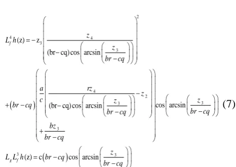
In this section, all simulations are performed with 0.1 Figure 3 shows 1,ˆ1with unsaturated control
signal and ˆ1 with the adaptive and non-adaptive saturation element. Figure 4 compares the energy of the
error
2 1 1 0ˆ
t dt
using the mentioned method showing that the proposed technique has a better performance in the sense of the mentioned index. In order to indicate the superiority of using the adaptive saturation element for all three methods and positive effect of using adaptive saturation on reducing the peaking phenomenon, Figure 5 shows 21 0
ˆ t
J dt
for each three methods. Ascan be observed, the proposed method has the minimum peak among them.
B. Stability Results
It was found that below of the critical value of the 0.065 , the high-gain observer with the non-adaptive saturation element becomes unstable. It is worth noting that through the unstable regime, ball drops from the wheel att 0.012sFigure 6 shows1and ˆ1when the adaptive structure for saturating control signal is used at the critical value of . As can be seen, ˆ1 tracks
1
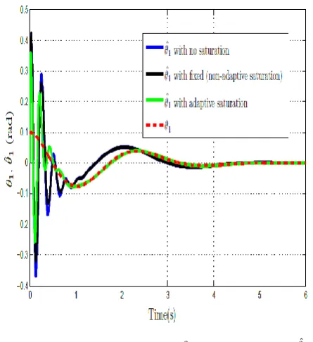
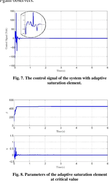
perfectly and the performance is maintained while other methods fail. Control signal is depicted in Figures 7 and the variation of the parameters of the adaptive saturation element, i.e.
and
are illustrated in Figure 8.Fig. 4.Comparison of the energy of the error among three methods.
Fig. 3.The red dashed line is1, the blue rigid line is ˆ1
when control signal is not restricted, the green and black rigid lines areˆ1when the adaptive and fixed
(non-adaptive) saturation elements are used, respectively. The slope and the height of the fixed saturation element are 1and 1, respectively. The initial value for the adaptive saturation height
5.CONCLUSION
The design process of adaptive saturation structure for attenuating peaking phenomenon in high-gain observers was addressed. The idea was successfully applied to controlling a Ball and Wheel system. By utilizing the Lyapunov stability theorem, the adaptation laws for tuning a smooth function as the saturation element were derived in a manner to make the time-derivative of the Lyapunov function negative semi-definite, where the asymptotic stability could be inferred through the LaSalle’s invariance theorem. In high-gain observers, the small positive parameter , whose reduction increases the convergence rate of the estimation error dynamics, may be viewed as a robustness tuning measure. It is worth noting, however, that choosing smaller may throw the system states outside the domain of attraction leading to system instability. It was shown that in comparison with the conventional scheme of the high-gain observer, i.e., with a fixed (non-adaptive) saturation element, the proposed
scheme may tolerate a smaller . This means that the proposed approach may provide a higher robustness for high-gain observers.
REFERENCE
[1] M. Farza, A. Sboui, E. Cherrier, and M. M’Saad, “High-gain observer for a class of time-delay nonlinear systems,” International Journal of Control, vol. 83, no. 2, pp. 273–280, February 2010.
[2] M.-T. Ho, Y.-W. Tu, and H.-S. Lin, “Controlling of ball and wheel system using full-state feedback linearization,” IEEE Control System Magazine, October 2009.
[3] J. C. Doyle and G. Stein, “Robustness with observers,” IEEE Transactions on Automatic Control, vol. 24, pp. 607 – 611, August 1979. [4] A. Saberi and P. Sannuti, “Observer design for
loop transfer recovery for uncertain dynamical systems,” IEEE Transactions on Automatic Control, vol. 35, no. 8, pp. 878–897, August 1990. [5] P. Dorl´eans, j. F. Massieu, and T. Ahmed-Ali,
“High-gain observer design with sampled measurements: application to inverted pendulum,”
Fig. 8.Parameters of the adaptive saturation element at critical value
Fig. 7.The control signal of the system with adaptive saturation element.
Fig. 6.The red dashed line is
1
, the blue continuous line is –when adaptive saturation element is used at
1
ˆ
. The initial condition for proposed adaptive law is set to (0)100.
International Journal of Control, vol. 84, no. 4, pp. 801–807, April 2011.
[6] Y. Li, X. Xia, and Y. Shen, “A high-gain-based global finite-time nonlinear observer,” International Journal of Control, vol. 86, no. 5, pp. 759–767, 2013.
[7] H. J. Sussmann and P. V. Kokotovic, “Peaking and stabilization,” IEEE Conference on Decision and Control, vol. 2, pp. 1379 – 1384, December 1989. [8] T. Mita, “On zeros and responses of linear
regulators and linear observers,” IEEE Transactions on Automatic Control, vol. 22, no. 3, pp. 423–428, June 1977.
[9] F. Esfandiari and H. K. Khalil, “Output feedback stabilization of fully linearized systems,” International Journal of Control, vol. 56, no. 3, pp. 1007–1037, December 1992.
[10] A. A. Ball and H. K. Khalil, “Analysis of a nonlinear high-gain observer in the presence of measurement noise,” American Control Conference, pp. 2584 – 2589, July 2011.
[11] H. K. Khalil, Nonlinear Systems. Upper Saddle River, New Jersey: Prentice Hall, 2002.
[12] J. H. Ahrens and H. K. Khalil, “Output feedback control using high-gain observers in the presence of measurement noise,” American Control Conference, vol. 5, pp. 4114 – 4119, July 2004.. [13] H. K. Khalil, “High-gain observer in nonlinear
feedback control,” International Conference on Control, Automation and Systems, pp. xlvii – lvii, October 2008.
![Fig. 1. The schematic overview of the ball and wheel system, adopted from [1]](https://thumb-us.123doks.com/thumbv2/123dok_us/8944563.1853931/3.595.276.543.76.522/fig-schematic-overview-ball-wheel-adopted.webp)