Multiple Target Tracking With a 2-D Radar Using the JPDAF Algorithm and Combined Motion Model

(1)

Multiple Target Tracking With a 2-D Radar Using the

JPDAF Algorithm and Combined Motion Model

Aliakbar Gorji Daronkolaeii, Mohammad Bagher Menhajii, Ali Doostmohammadiiii

i Corresponding Author, Ali A.Gorji is with the Department of Electrical And Computer Engineering, McMaster University, Hamilton, Canada (e-mail: [email protected]).

ii

M. B. Menhaj is with the Department of Electrical Engineering, Amirkabir University of Technology, Tehran, Iran (e-mail:[email protected]). iii

Ali Doostmohammadi is with the Department of Electrical Engineering, Amirkabir University of Technology, Tehran, Iran .

ABSTRACT

Multiple target tracking (MTT) is taken into account as one of the most important topics in tracking targets with radars. In this paper, the MTT problem is used for estimating the position of multiple targets when a 2-D radar is employed to gather measurements. To do so, the Joint Probabilistic Data Association Filter (JPDAF) approach is applied to tracking the position of multiple targets. To characterize the motion of each target, two models are used. First, a simple near constant velocity model is considered and then to enhance the tracking performance, specially, when targets make maneuvering movements a variable velocity model is proposed.In addition, a combined model is also proposed to mitigate the maneuvering movements better. This new model gives an advantage to explore the movement of the maneuvering objects which is common in many tracking problems. Simulation results show the superiority of the new motion model and its effect in the tracking performance of multiple targets.

KEYWORDS

Multiple target tracking, JPDAF algorithm, data association, maneuvering movement

1. INTRODUCTION

The problem of estimating the position of a target in physical environment is an important problem in the military field. Indeed, because of the intrinsic error embedded in the data collected by measurement sensors, here range and bearing finders, some operations should be conducted on the crude data to reach more accurate knowledge about the position of a target. Nowadays, various algorithms are proposed to modify the accuracy of localization algorithms.

In the field of target tracking, the Kalman filter approach [1] plays a significant role. This approach uses a suggested model describing the target’s movement and the measurements collected by a 2-D radar and, then, provides an accurate estimation of the target’s position. Now, the Kalman filter is greatly used in many tracking problems [2]. Although this filter has provided a general strategy to solve localization problems, it suffers from some weaknesses. The most significant problem of the Kalman method is its weakness to the state estimation of many real systems in the presence of severe nonlinearities. Actually, in general nonlinear systems, the posterior probability density function of states given measurements cannot be presented by a Gaussian density

function and, therefore, the Kalman method may result in unsatisfactory responses. Moreover, the Kalman filter is very sensitive to the initial conditions of states. Accordingly, Kalman based methods do not provide accurate results in many common global localization problems.

More recently, particle filters have been introduced to estimate non-Gaussian, non-linear dynamic processes [5].The key idea of particle filters is to represent the state by sets of samples (or particles). The major advantage of this technique is that it can represent multi-modal state densities, a property which has been shown to increase the robustness of the underlying state estimation process. Moreover, particle filters are less sensitive to the initial values of states than the Kalman method is. This problem is very considerable in applications in which the initial values of states are not known such as global localization problems. The aforementioned power of particle filters in the state estimation of nonlinear systems has made them be applied with great success to different state estimation problems including visual tracking [6], mobile robot localization [7], control and scheduling [8], target tracking [9] and dynamic probabilistic networks [10].

(2)

introduced as tracking targets’ position by data received from a 2-D radar. Although this problem appears similar to the common localization algorithms in which the dynamical model of the target is known, the traditional approaches cannot be used because the radar does not have access to the internal sensors’ data of each target used in localization algorithms to predict the future position of the target. Moreover, using the particle filter to estimate the position of all targets, known as combined state space, is not tractable because the complexity of this approach grows exponentially with the number of objects being tracked.

To resolve the problem of the lack of internal sensors’ data, various motion models have been proposed. The simplest model proposed is the near constant velocity model. This model has been greatly used in many tracking applications such as aircraft tracking [11], people tracking [12] and some other target tracking applications [13]. Besides this model, some other structures have been proposed usable in some other special applications. Near constant acceleration model is a modified version of the previous model which can be applied to tracking maneuvering objects [14]. Also, interactive multiple model (IMM) filters represent another tool to track the movement of highly maneuvering objects where the former proposed approaches are not reliable [15].

Recently, many strategies have been also proposed in the literature to address the difficulties associated with multitarget tracking. The key idea of the literature is to estimate each object’s position separately. To do so, the measurements should be assigned to each target. Therefore, data association has been introduced to relate each target to its associated measurements. By combining data association concept with filtering and state estimation algorithms, the multiple target tracking issue can be dealt with easier than applying state estimation procedure to the combined state space model. Among the various methods, Joint Probabilistic Data Association Filter (JPDAF) algorithm is taken into account as one of the most attractive approaches. The traditional JPDAF [16] uses Extended Kalman Filtering (EKF) joint with the data association to estimate states of multiple objects. However, the performance of the algorithm degrades as the nonlinearities become more severe. To enhance the performance of the JPDAF against the severe nonlinearity of dynamical and sensor models, recently, strategies have been proposed to combine the JPDAF with particle techniques known as Monte Carlo JPDAF, to accommodate general nonlinear and non-Gaussian models [17]. The newer versions of the above-mentioned algorithm use an approach named as soft gating to reduce the computational cost which is one of the most serious problems in online tracking algorithms [17]. Besides the Monte Carlo JPDAF algorithm, some other methods have been proposed in the literature. In [17], a comprehensive

survey has been presented on the most well-known algorithms applicable in the field of multiple target tracking.

In this paper, the Monte Carlo JPDAF algorithm is used for the multiple target tracking problem. As a modification to the recent literature, different motion models are tested to evaluate the performance of tracking. Besides the traditional near constant velocity model, we will test the efficiency of the other two models as well in the paper. First, a variable velocity model is used to characterize the movement of targets. Then, we propose a combined approach in which the motion model is a linear combination of constant and variable velocity models. In addition, a simple algorithm is represented to determine the weights assigned to each motion model. It is shown that some information of the JPDAF algorithm can be used to determine the aforementioned factors. The goal, here, is to justify the efficiency of the JPDAF algorithm using combined model compared with each individual model.

The rest of this paper is organized as follows. Section II describes the Monte Carlo JPDAF algorithm for multiple target tracking. The JPDAF for multiple target tracking is the topic of section III. In this section, we will present how the motion of targets in a real environment can be described. To do so, near constant velocity and acceleration models are introduced to describe the movement of mobile targets. Then, it will be shown how data received from a 2-D radar can be used for tracking moving objects. In section IV, various simulation results are presented to support the performance of the algorithm. In this section, the maneuvering movement of the target is also considered. The results easily approve the suitable performance of the JPDAF algorithm in tracking the motion of mobile targets in the simulated environment. Finally, section V concludes the paper.

2. THE JPDAFALGORITHM FOR MULTIPLE TARGET TRACKING

This section presents the JPDAF algorithm considered as the most successful and widely applied strategy for multi-target tracking under data association uncertainty. The Monte Carlo version of the JPDAF algorithm uses common particle filter approach to estimate the posterior density function of states given measurements

p

(

x

_t

|

y

₁_:_t

)

.

Now, consider the problem of tracking N

objects.

x

_tkdenotes the state of these objects at time t

where k=1,2,..,N is the the target number. Furthermore, the movement of each target can be considered by a general nonlinear state space model as follows:

t t

t

f

x

v

x

₊_`

=

(

)

+

t t

t

g

x

w

(3)

where

v

_t and

w

_tare white noises with the covariance

matrices Q and R, respectively. Also, in the above equation, f and g are the general nonlinear functions representing the dynamic behavior of the target and the sensor model. The JPDAF algorithm recursively updates the marginal filtering distribution for each target

)

|

(

x

_tk

y

₁_:_t

p

, k=1,2,..,N instead of computing the joint

filtering distribution

p

(

X

_t

|

y

₁_:_t

)

,

X

_t

=

x

_t1

,...,

x

_tN. To compute the above distribution function, some points have to be taken into consideration as follows:

- It is very important to know how to assign each target’s state to a measurement. Indeed, the sensor provides a set of measurements at each time step. The source of these measurements can be the targets or the disturbances also known as clutters. Therefore, a special procedure is needed to assign each target to its associated measurement. This procedure is designated as Data Association considered as the key stage of the JPDAF algorithm which is described in the next sections.

- Because the JPDAF algorithm recursively updates the estimated states, a recursive solution should be applied to update states at each sample time. Traditionally, Kalman filtering has been a strong tool for recursively estimating states of the targets in multi-target tracking scenario. Recently, particle filters joint with the data association strategy have provided better estimations, specially, when the sensor model is nonlinear.

With regard to the above points, the following sections describe how particle filters paralleled with the data association concept can deal with the multi-target tracking problem.

A. The Particle Filter For Online State Estimation

Consider the problem of online state estimation as computing the posterior probability density

function

p

(

x

_tk

|

y

₁_:_t

)

. To provide a recursive formulation for computing the above density function, the following stages are presented:

- Prediction stage: the prediction step is done independently for each target as:

∫

−

− − − − −

=

k t

x

k t t k t k t k t t

k

t

y

p

x

p

x

y

dx

x

p

1

1 1 1 1 1

:

1

)

(

|

)

(

|

)

|

(

(2)

- Update stage: the update step can be described as follows:

)

|

(

)

|

(

)

|

(

x

_tk

y

₁_:_t

∝

p

y

_t

x

_tk

p

x

_tk

y

₁_:_t₋₁

p

(3)

The particle filter estimates the probability density

function

(

k

|

₁_:_t₋₁

)

t

y

x

p

by sampling from a specific

distribution function as follows:

∑

=

−

=

−

N

i

i t t i t t

k

t

y

w

x

p

1 1 :

1

)

~

(

)

|

(

δ

(4)

where i=1,2,...,N is the sample number,

w

~

_t is the

normalized importance weight and

δ

is the delta dirac

function. In the above equation, the state

x

_ti is sampled

from the proposal density function

(

|

k₁

,

₁_:_t

)

t k

t

x

y

x

q

₋ . By

substituting the above equation in (2) and the fact that the states are drawn from the proposal function q, the recursive equation for the prediction step can be written as follows:

)

,

|

(

)

|

(

: 1 , 1

, 1 1

t i k t k t

i k t k t i

t i t

y

x

q

x

p

− − −

=

α

(5)

where

x

_tk,i

is the i-th sample of

x

_tk.Now, by using (3) the

update stage can be expressed as the recursive adjustment of importance weights as follows:

)

|

(

_t _ti

i t i

t

p

y

x

w

=

α

(6)

By repeating the above procedure at each time step the sequential importance sampling (SIS) for online state estimation is presented below:

The SIS Algorithm

1. For i=1: N initialize the states

x

₀i, prediction weights

α

₀i and importance weights

w

₀i.

2. At each time step t proceed the following stages: 3. Sample the states from the proposal density

function as follows:

)

,

|

(

~

_t _ti₁ ₁_:_t

i

t

q

x

y

x

₋ (7)

4. Update prediction weights using (5). 5. Update importance weights using (6). 6. Normalize importance weights as follows:

∑

=

_N

i i t i t i t

w

1

~

(8)

7. Set t=t+1 and go to step 3.

In the above, for simplicity, the index, k, has been eliminated.

(4)

the SIR algorithm as follows:

The SIR Algorithm

1. For i=1: N initialize the states

x

₀i, prediction weights

α

₀i and importance weights

w

₀i.

2. At each time step t, do the following:

3. perform the SIS algorithm to sample states

x

_ti and

compute normalized importance weights

w

~

_ti.

4. Check the re-sampling criterion:

a. If

N

_eff

>

thresh

follow SIS stages

Else

b. Implement residual-resampling approach to multiply/suppress states with high/low weights. c. Set new normalized importance weights as

N

w

~

_ti

=

1

. 5. Set t=t+1 and go to step 3.

In above,

N

_effis a criterion checking the degeneracy of

algorithm which can be written as:

∑

=

_N

i i t eff

w

N

1 2

)

~

(

1

(9)

In [19], a comprehensive discussion has been made on how to implement the residual re-sampling stage.

Besides the SIR algorithm, some other approaches have been proposed in the literature to enhance the quality of the SIR algorithm such as Markov Chain Monte Carlo particle filters, Hybrid SIR and auxiliary particle filters [20]. Although these methods are more accurate than the common SIR algorithm, some other problems such as the computational cost are the most significant reasons that, in many real time applications such as online tracking, the traditional SIR algorithm is applied to recursive state estimation.

B. Data Association

In the last section, the SIR algorithm was presented for online state estimation. However, the major problem of the proposed algorithm is how to compute the likelihood

function

(

|

k

)

t

x

y

p

. To do so, an association should be

made between the measurements and targets. Briefly, the association can be categorized into target to measurement and measurement to target:

Definition 1: A target to measurement association

denoted as (

T

→

M

) is defend by

{

r

,

M

c

,

M

T

}

~

₌

λ

where

r

~

=

r

~

₁

,...,

r

~

_Kwith: If the k-th target is undetected

If the k-th target has

generated the j-th measurement

0

k

r

j

⎧

⎪

= ⎨

⎪

⎩

where j=1,2,...,m and m is the number of measurements at each time step and k=1,2,..,K which K is the number of targets.

Definition 2: in a similar fashion, the measurement to

target association (

M

→

T

) is defined by

{

r

,

M

c

,

M

T

}

=

λ

where

r

=

r

₁

,...,

r

_mand

r

_j is given below.

If the j-th measurement

is not associated with any target

If the j-th target is

associated with the k-th target

0

j

r

k

⎧

⎪

= ⎨

⎪

⎪⎩

In the both above equations,

m

_Tis the number of

measurements due to targets and

m

_cis the number of

clutters. It is very easy to show that both definitions are equivalent, however the dimension of the target to measurement association is less than that of the measurement to target association. Therefore, in this paper, the target to measurement association is used.

Now, the likelihood function for each target can be written as:

∑

=

+

=

m

i

k t i t i k

t

x

p

y

x

y

p

1 0

)

|

(

)

|

(

β

(10)

In the above equation,

β

iis defined as the probability

that the

i

−

th

measurement is assigned to the

k

−

th

target. Hence,

β

i is written as:

)

|

~

(

_k ₁_:_t

i

y

i

r

p

=

β

(11)

Before elaborating more on the above equation, the following definition is needed.

Definition 3: We define the set

Λ

~

as all possible assignments which can be made between measurements and targets.

For example, consider a 3-target tracking problem. Assume that following associations are recognized between targets and measurements:

0 ,

3 ,

1

₂ ₃

1

=

r

=

r

=

r

Now, the set

Λ

~

can be listed as given in table I.

TABLE 1

ALLPOSSIBLEASSOCIATIONSBETWEENTARGETSAND MEASUREMENTSFOREXAMPLE1

TARGET 1 TARGET 2 TARGET 3

(5)

Here, 0 means that the target has not been detected. By using the above definition, Eq.(11) can be rewritten as:

∑

∈Λ =

=

t _r _j t t

k k t t

y

p

y

j

r

p

₁_: ~ ~_,~

|

₁_:

)

~

(

)

|

~

(

_λ

λ

(12)

The right side of the above equation is written as follows:

)

~

(

)

~

,

|

(

)

(

)

~

,

(

)

~

,

|

(

)

|

~

(

1 : 1 : 1 1 : 1 1 : 1 : 1 t t t t t t t t t t t t

p

y

p

y

p

y

p

y

p

y

p

λ

− − −

₌

=

(13)

where we have used the fact that the association vector

t

λ

~

is not dependent on the history of measurements. Each of the density functions in the right side of the above equation is stated as follows:

-

p

(

λ

~

_t

)

The above density function becomes

)

(

)

(

)

,

|

~

(

)

,

~

(

)

~

(

T c T c t T c t t

M

p

M

p

M

r

p

M

r

p

λ

=

(14)

The computation of each density function in the right side of the above equation is straightforward as fully discussed in [17].

-

p

(

y

_t

|

y

₁_:_t₋₁

,

λ

~

_t

)

Because the targets are supposed to be independent, the above density function can be written as follows:

(

)

_∏

(

)

Γ ∈ − − −

=

j t j t r M t t

t

y

V

p

y

p

c tj

1 : 1 max 1 :

1

)

|

~

,

|

(

λ

(15)

where

V

_maxis the maximum volume which is in the line of sight of the sensors,

Γ

is the set of all valid measurement to target associations and

p

rtj

(

y

_t

|

y

₁_:_t₋₁

)

_is the predictive likelihood for the

r

_tj

−

th

target.

Now, consider

r

_tj

=

k

. The predictive likelihood for the k-th target can be formulated as:

∫

−

=

t tk

k t k t j t t j t k

dx

y

x

p

x

y

p

y

p

(

|

₁_: ₁

)

(

|

)

(

|

₁_: ₁

)

(16)

Both density functions in the right hand side of the above equation are estimated using the samples drawn from the proposed density function. However, the main problem is how to determine the association between measurements (

y

_t) and targets. To do so, a soft gating method is

proposed in the following algorithm:

Soft Gating

1. Consider

x

_ti,k, i=1,2,…,N, as samples drawn from the proposed density function.

2. For j=1:m, do the following steps for the j-th measurement.

3. For k=1:K, do the following steps:

4. Compute

µ

k_jas follows:

∑

=

N i k i t k i t k

j

g

x

1 , ,

)

(

~

α

µ

(17)

where g is the sensor model and

α

~

_tk is the normalized

weight as presented in the SIR algorithm. 5. Compute

σ

k_j as:

(

)(

)

∑

=

−

+

=

N i T k j k i t k j k i t k i t k

j

R

g

x

g

x

1 , , ,

)

(

)

(

~

_µ

α

σ

(18)

6. Compute the distance to the j-th target by:

(

) ( ) (

k

)

j j t k j T k j j t

j

y

d

2

=

−

µ

σ

−1

−

µ

2

1

(19)

7. If

d

2_j

<

ε

, assign the j-th measurement to the k-th target.

It is easy to show that the predictive likelihood given in (16) can be approximated by:

(

k k

)

t j t k

N

y

p

(

|

1:−1

)

≈

µ

,

σ

(20)

where

N

(

µ

k

,

σ

k

)

is a normal distribution with mean

k

µ

and the covariance matrix

σ

k. By computing the predictivelikelihood, the likelihood density function is easily estimated. In the next subsection, the JPDAF algorithm is presented formulti-target tracking problem.

C. The JPDAF Algorithm

The mathematical foundations of the JPDAF algorithm were discussed in the last sections. Now, we are ready to propose the full JPDAF algorithm for the problem of multiple target tracking. To do so, each target is characterized by the dynamical model introduced in (1). The JPDAF algorithm is presented below.

The JPDAF Algorithm

1. Initialization: initialize states for each target as

x

₀i,k where i=1,2,..,N and k=1,2,...,K, the predictive importance weights

α

₀i,k and importance weights

k i

w

₀, .

2. At each time step t, proceed as: 3. For i=1:N, do the following steps.

4. For k=1:K, conduct the following procedures for each target.

5. Sample the new states from the proposed density function as follows:

(

t

)

k i t t k i

t

q

x

y

x

, ₁_:

1

,

_~

_|

_,

−

(6)

6. Update the predictive importance weights as:

(

)

(

t

)

k i t k i t

k i t k i t k i t k i t

y

x

q

x

p

: 1 ,

1 ,

, 1 , ,

1 ,

,

|

− − −

=

α

(22)

Then, normalize the predictive importance weights.

7. Use the sampled states and new observations,

y

_t, to constitute the association vector for each target

as

R

k

=

{

j

|

0 ≤

j

≤

m

,

y

_j

→

k

}

where (

→

k

) refers to the association between the k-thtarget and the j-th measurement. To do so, use the soft gating procedure described in the previous subsection. 8. Constitute all possible associations for the targets

and establish the set

Γ

~

as described in definition 3.

9. Use (13) and compute

β

i for each measurement where l=1,2,..,m and m is the number of measurements.

10. Use (10) to compute the likelihood ratio for each

target as

p

(

y

_t

|

x

_ti,k

)

.

11. Compute the importance weights for each target as:

(

ik

)

t t k i t k i

t

p

y

x

w

,

=

α

,

|

, (23)

Then, normalize the importance weights as follows:

∑

=

_N

i k i t k i t k i t

w

, , ,

~

(24)

12. Proceed with the re-sampling stage. To do so, implement the similar procedure described in the SIR algorithm. Afterwards, for each target the resampled states can be presented as follows:

{

}

⎭

⎬

⎫

⎩

⎨

⎧

→

mi k

t k

i t k i

t

x

N

x

w

~

,

_,

,

1 _,

(), (25)

13. Set the time as t=t+1 and go to step 3.

In the next section, the JPDAF algorithm for multiple case can be used for multiple target tracking. In addition, some well-known motion models are then presented to track the motion of a mobile target.

3. THE JPDAF ALGORITHM FOR MULTIPLE TARGET

TRACKING WITH A 2-D RADAR

Now, we want to use the JPDAF algorithm for the problem of multiple target tracking with a 2-D radar. To do so, Radar systems use modulated waveforms and directive antennas to transmit Electromagnetic energy into a specific volume in space to search for targets. Objects (targets) within a search volume will reflect portions of this energy (radar returns or echoes) back to the radar. These echoes are then processed by the radar receiver to

extract target information such as range, velocity, angular position and other target identifying characteristics. To estimate the position of each target by data collected via a 2-D radar, we need a motion model to describe the behavior of the target. The simplest method is near constant velocity model, presented as:

[

t t t t

]

t

t t t

y

x

X

Bu

AX

X

=

+

=

+1

(26)

where the system matrixes are defined as:

⎟

⎠

⎞

⎜

⎝

⎛

=

⎟⎟

⎟

⎠

⎞

⎜⎜

⎜

⎝

⎛

=

s s s s

s s

T

B

T

A

0

2

0

2

1

0

1

0

1

0

1

2 2

(27)

where

T

_s refers to the sample time. In the above

equations,

u

_t is white noise with zero mean and an

arbitrary covariance matrix. Because the model is considered as a near constant velocity, the covariance of the additive noise cannot be so large. Indeed, this model is suitable for the movement of targets with a constant velocity, which is common in many applications such as commercial aircraft path tracking [8] and people tracking [12].

The movement of a target can be modeled by the above model in many conditions. However, in some special cases, the targets’ movement cannot be characterized by a simple near constant velocity model. For example, in many problems, targets may conduct a maneuvering movement. Therefore, the motion trajectory of the target is so complex that the elementary constant velocity model will not result in satisfactory responses. To overcome this problem, the variable velocity model is proposed. The key idea behind this model is to use the target’s acceleration as another state variable which should be estimated as well as computing the velocity and position of the target. In other words, the new state vector is defined as,

[

y

]

t t t x t t t

t

x

a

y

a

X

=

, where

a

_txand

a

_ty

(7)

⎟

⎠

⎞

⎜

⎝

⎛

=

⎟

⎠

⎞

⎜

⎝

⎛

−

=

3 3 2 2 1 1 2 2 1 1

0

0 )

exp(

0

0 )

exp(

0

1

0

1

0

1

0

1 b

b

B

T

a

T

a

T

A

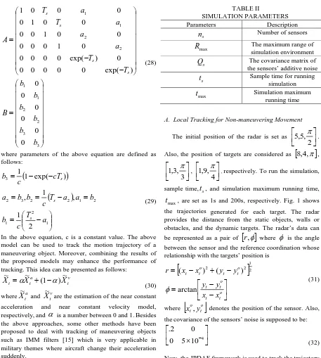
s s s s (28)

where parameters of the above equation are defined as follows:

(

)

(

)

⎟⎟

⎠

⎞

⎜⎜

⎝

⎛

₋

=

−

=

−

=

1 2 1 2 1 2 2 3 2 3

2

1 ,

)

exp(

1

1 a

T

c

b

a

T

c

b

a

cT

c

b

s s s (29)

In the above equation, c is a constant value. The above model can be used to track the motion trajectory of a maneuvering object. Moreover, combining the results of the proposed models may enhance the performance of tracking. This idea can be presented as follows:

v t a

t

X

~

=

α

~

+

(

1 −

α

)

~

(30)

where

X

~

_ta and

X

~

_tvare the estimation of the near constant

acceleration and near constant velocity model, respectively,and

α

is a number between 0 and 1.Besides the above approaches, some other methods have been proposed to deal with tracking of maneuvering objects such as IMM filters [15] which is very applicable in militarythemes where aircraft change their acceleration suddenly.

4. SIMULATION RESULTS

To evaluate the efficiency of the JPDAF algorithm, a 3- target tracking scenario is considered. To prepare the scenario and implement simulations, the parameters are presented for targets structure and simulation environment as TABLE II.

Now, the following experiments are conducted to evaluate the performance of the JPDAF algorithm in various situations.

TABLE II

SIMULATION PARAMETERS

Parameters Description

s

n

Number of sensors

max

R

The maximum range of

simulation environment

s

Q

The covariance matrix of

the sensors’ additive noise

s

t

Sample time for running

simulation

max

t

Simulation maximum

running time

A. Local Tracking for Non-maneuvering Movement

The initial position of the radar is set as

⎥⎦

⎤

⎢⎣

⎡

2 ,

5 ,

5 π

.

Also,the position of targets are considered as

[

8 ,

4 ,

π

]

,

⎥⎦

⎤

⎢⎣

⎡

3 ,

1 π

,

_⎢⎣

⎡

_⎥⎦

⎤

4 ,

9 ,

1 π

, respectively. To run the simulation,

sampletime,

t

_s, and simulation maximum running time,

max

t

, areset as 1s and 200s, respectively. Fig. 1 shows the trajectories generated for each target. The radar provides the distance from the static objects, walls or obstacles, and the dynamictargets. The radar’s data can be represented as a pair of

[ ]

r

,

φ

where

φ

is the angle between the sensor and the referencecoordination whose relationship with the targets’ position is

[

]

⎥

⎦

⎤

⎢

⎣

⎡

−

=

−

+

−

=

o t t o t t o t t o t t

x

y

x

r

arctan

)

(

)

(

2 1 2 2

φ

(31)

where

[

x

_to

,

y

_to

]

denotes the position of the sensor. Also, thecovariance of the sensors’ noise is supposed to be:

⎥

⎦

⎤

⎢

⎣

⎡

×

₁₀

−4

5

0

2 .

(32)

Now, the JPDAF framework is used to track the trajectory of each target. In this simulation, the clutters are assumed to be uniformly distributed over the total volume of the environment. To apply the near constant velocity model as described in (27), the initial value of the velocity is chosen uniformly between 1 and -1 as follows:

)

1 ,

1 (

)

1 ,

1 (

−

=

−

=

u

y

u

x

t t

(33)

(8)

with 500 particles for each target’s tracking. Simulation results justify the ability of the JPDAF algorithm in modifying the intrinsic error embedded in the data collected from the measurement sensor.

Fig. 1. The generated trajectory for targets

Fig. 2. The estimated trajectory using the JPDAF algorithm

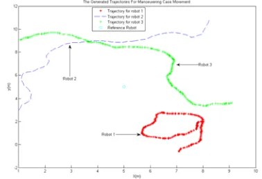
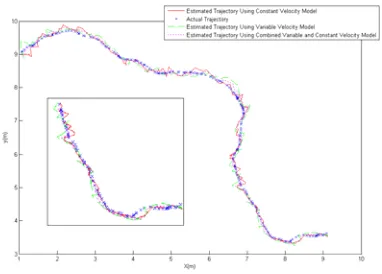
B. Local Tracking for Maneuvering Movement

Now, consider a maneuvering movement for each target. Therefore, a variable velocity model is considered for each target’s movement. Fig. 3 shows the generated trajectory for each target. Now, we apply the JPDAF algorithm for tracking each target’s position. To do so, 3 approaches are implemented. Near constant velocity model, near constant acceleration model and combined model described in the last section are used to estimate the states of the targets. Figs. 4-6 show the results for each target separately. To compare the efficiency of each strategy, the obtained error is presented for each approach in tables III, IV where the following criterion is used for estimating the error:

{

_t _t

}

t t

t

t t

z

x

y

t

z

e

,

)

~

(

max 1

2 max

=

−

=

∑

= (32)

The results show better performance of the combined method compared with the other approaches.

5. CONCLUSIONS

In this paper, the JPDAF algorithm was fully developed for multiple target tracking. After introducing the mathematical basis of the JPDAF algorithm, we showed how to apply the JPDAF algorithm to the problem of multiple target tracking; this led to three different models proposed in the paper. Near constant velocity model, near constant acceleration model were first described and, then, a combination of the two former approaches was presented to enhance the tracking accuracy. Afterwards, simulation results were carried out in two different scenarios. First, tracking the non-maneuvering motion of targets was explored. Later, the JPDAF algorithm was tested on tracking the motion of targets with maneuvering movements. Simulation results showed that the combined approach provides better performance than the other two proposed strategies.

Fig. 3. The generated trajectory for maneuvering targets

Fig. 4. The estimated trajectory for target 1

TABLE III THE ERROR FOR ESTIMATING

x

_t

Robot Num Constant Acceleration

Constant Velocity

Combined

1 .0045 .0046 .0032

2 .0112 .0082 .005

(9)

TABLE IV THE ERROR FOR ESTIMATING

y

_t

Robot Num Constant Acceleration

Constant Velocity

Combined

1 .0082 .009 .0045

2 .0096 .0052 .005

3 .0073 .0077 .0042

6. REFERENCES

[1] R. E. Kalman, and R. S. Bucy, New Results in Linear Filtering and Prediction, Trans. American Society of Mechanical Engineers, Series D, Journal of Basic Engineering, Vol. 83D, pp. 95–108, 1961.

[2] Branko Ristic, Sanjeev Arulampalam, and Neil Gordon, Beyond the Kalman Filter: Particle Filters for Tracking Applications, Artech House, Boston, London, 2004.

[3] R. Siegwart and I. R. Nourbakhsh, Intoduction to Autonomous Mobile Robots, MIT Press, 2004.

[4] A. Howard, Multi- robot Simultaneous Localization and Mapping using Particle Filters, Robotics: Science and Systems I, pp. 201– 208, 2005.

[5] N.J. Gordon, D.J. Salmond, and A.F.M. Smith, A Novel Approach to Nonlinear/non-Gaussian Bayesian State Estimation, IEE Proceedings F, 140(2):107–113, 1993.

[6] M. Isard, and A. Blake, Contour Tracking by Stochastic Propagation of Conditional Density, In Proc. of the European Conference of Computer Vision, 1996.

[7] D. Fox, S. Thrun, F. Dellaert, andW. Burgard, Particle Filters for Mobile Robot Localization, Sequential Monte Carlo Methods in Practice. Springer Verlag, New York, 2000.

[8] C. Hue, J. P. L. Cadre, and P. Perez, Sequential Monte Carlo Methods for Multiple Target Tracking and Data Fusion, IEEE Transactions on Signal Processing, Vol. 50, NO. 2, February 2002. [9] B. Ristic, S. Arulampalam, and N. Gordon, Beyond the Kalman

Filter, Artech House, 2004.

[10] K. Kanazawa, D. Koller, and S.J. Russell, Stochastic Simulation Algorithms for Dynamic Probabilistic Networks, In Proc. of the 11th

Annual Conference on Uncertainty in AI (UAI), Montreal, Canada, 1995.

[11] F. Gustafsson, F. Gunnarsson, N. Bergman, U. Forssell, J. Jansson, R. Karlsson, and P. J. Nordlund, Particle Filters for Positioning, Navigation, and Tracking, IEEE Transactions on Signal Processing, Vol. 50, No. 2, February 2002.

[12] D. Schulz, W. Burgard, D. Fox, and A. B. Cremers, People Tracking with a Mobile Robot Using Sample-based Joint Probabilistic Data Association Filters, International Journal of Robotics Research (IJRR), 22(2), 2003.

[13] M. S. Arulampalam, S. Maskell, N. Gordon, and T. Clapp, A Tutorial on Particle Filters for Online Nonlinear/Non-Gaussian Bayesian Tracking, IEEE Transactions on Signal Processing, Vol. 50, No. 2, February 2002.

[14] N. Ikoma, N. Ichimura, T. Higuchi, and H. Maeda, Particle Filter Based Method for Maneuvering Target Tracking, IEEE International Workshop on Intelligent Signal Processing, Budapest, Hungary, May 24-25, pp.3– 8, 2001.

[15] R. R. Pitre, V. P. Jilkov, and X. R. Li, A comparative study of multiple model algorithms for maneuvering target tracking, Proc. 2005 SPIE Conf. Signal Processing, Sensor Fusion, and Target Recognition XIV, Orlando, FL, March 2005.

[16] T. E. Fortmann, Y. Bar-Shalom, and M. Scheffe, Sonar Tracking of Multiple Targets Using Joint Probabilistic Data Association, IEEE Journal of Oceanic Engineering, Vol. 8, pp. 173–184, 1983. [17] J. Vermaak, S. J. Godsill, and P. Perez, Monte Carlo Filtering for

Multi-Target Tracking and Data Association, IEEE Transactions on Aerospace and Electronic Systems, Vol. 41, No. 1, pp. 309–332, January 2005.

[18] O. Frank, J. Nieto, J. Guivant, and S. Scheding, Multiple Target Tracking Using Sequential Monte Carlo Methods and Statistical Data Association, Proceedings of the 2003 IEEE/IRSJ, International Conference on Intelligent Robots and Systems, Las Vegas, Nevada, October 2003.

[19] Jao F. G. de Freitas, Bayesian Methods for Neural Networks, PhD thesis, Trinity College, University of Cambridge, 1999.