in the population sciences published by the Max Planck Institute for Demographic Research Konrad-Zuse Str. 1, D-18057 Rostock · GERMANY www.demographic-research.org
DEMOGRAPHIC RESEARCH
VOLUME 16, ARTICLE 3, PAGES 59-96
PUBLISHED 30 JANUARY 2007
http://www.demographic-research.org/Volumes/Vol16/3/ DOI: 10.4054/DemRes.2007.16.3
Research Article
The proximate determinants of fertility
and birth intervals in Egypt:
An application of calendar data
Angela Baschieri
Andrew Hinde
© 2007 Baschieri & Hinde
This open-access work is published under the terms of the Creative Commons Attribution NonCommercial License 2.0 Germany, which permits use, reproduction & distribution in any medium for non-commercial purposes, provided the original author(s) and source are given credit.
1 Introduction 60
2 Background and conceptual framework 62
3 Data and sample 67
4 Method 71
5 Results 73
5.1 ‘Proximate’ and ‘socio-economic’ models 75
5.2 Effect of length of first interval and contraception on the second birth interval
83
5.3 Unobserved heterogeneity 84
6 Conclusion 91
7 Acknowledgments 92
The proximate determinants of fertility and birth intervals in Egypt:
An application of calendar data
Angela Baschieri 1
Andrew Hinde 2
Abstract
In this paper we use calendar data from the 2000 Egyptian Demographic and Health Survey (DHS) to assess the determinants of birth interval length among women who are in union. We make use of the well-known model of the proximate determinants of fertility, and take advantage of the fact that the DHS calendar data provide month-by-month data on contraceptive use, breastfeeding and post-partum amenorrhoea, which are the most important proximate determinants among women in union. One aim of the analysis is to see whether the calendar data are sufficiently detailed to account for all non-random variation among individual women in birth interval duration, in that once they are controlled, the effect of background social, economic and cultural variables is not statistically significant. The results suggest that this is indeed the case, especially after a random effect term to account for the unobserved proximate determinants is included in the model. Birth intervals are determined mainly by the use of modern methods of contraception (the IUD being more effective than the pill). Breastfeeding and post-partum amenorrhoea both inhibit conception, and the effect of breastfeeding remains even after the period of amenorrhoea has ended.
1
Centre for Population Studies, London School of Hygiene and Tropical Medicine, 49-51 Bedford Square, London, WC1B 3DP, United Kingdom. E-mail: [email protected]
2
1. Introduction
It is now almost 30 years since John Bongaarts observed that the social, economic and cultural factors which influence fertility operate through what he called ‘proximate determinants’ (Bongaarts 1978). Changes in fertility are the direct result entirely of changes in these proximate determinants, which thus mediate the effect of changes in social, economic and cultural factors. This idea was not original to Bongaarts: 50 years ago Kingsley Davis and Judith Blake (Davis and Blake 1956) described the concept of ‘intermediate variables’ as a set of ‘factors through which and only through which, social, economic, and cultural conditions can affect fertility’ (Bongaarts 1982, p. 179). It was Bongaarts, however, who formalised the idea into a quantifiable model.
Using aggregate analysis with countries as units of analysis, Bongaarts (1982) demonstrated that, as the model posits, virtually all non-random variation in fertility is captured by differences in the proximate determinants. However, similar studies using individual-level data to analyse birth intervals have reached different results, and many authors have still found direct effects of social and economic variables on birth interval durations. Since, according to the model, the proximate determinants are exhaustive determinants of fertility outcomes, the existence of these residual direct effects has been explained by saying that the measurement of the proximate determinants is incomplete or inaccurate.
The most common set of data used to study fertility differentials in developing countries are the Demographic and Health Surveys (DHSs). These are large, nationally representative sample surveys collected for many countries around the world which provide information about fertility and family planning, including knowledge and current use of contraceptive methods, and detailed fertility histories with records of children’s birth and death dates. Recent DHSs have also collected monthly calendar data, which comprise a longitudinal record of contraceptive use, breastfeeding and post-partum amenorrhoea for countries with relatively high contraceptive use. Although these calendar data provide unusually detailed information, few studies have hitherto used them (Curtis 1997, Curtis and Blanc 1997, Magnani, Rutenberg and McCann 1996, Steele and Curtis 2003, Steele, Curtis and Choe 1999, Zhang, Tsui and Suchindran 1999).
12). Leone (2002) performed a similar analysis using DHS data on current contraceptive use for north-east Brazil in 1991 and data from the calendar in the 1996 Brazilian DHS on current use at the time of the 1991 DHS and found similarly reassuring results. Strickler et al. (1997) had the unique opportunity to use data from 1995 Morocco Panel Survey to evaluate the reliability of the contraceptive history data collected in the calendar of the 1992 DHS. The Panel Survey consisted of a sub-sample of respondents from the DHS calendar. Both surveys included a five-year calendar, and the two calendars overlap for the period 1990-92. They found that the reporting of contraceptive use was fairly reliable, though data on contraceptive discontinuation and on complex histories were less so. Overall, their results suggest that the contraceptive use data are fairly robust, although estimates of contraceptive failure rates are likely to be less accurate than estimates of prevalence.
According to Bongaarts’s (1982) framework, all the important variation in fertility is captured by variation by the proximate determinants of fertility. Therefore if we have good enough individual-level data on contraceptive use, breastfeeding and post-partum amenorrhoea and the other proximate determinants, we should be able to capture all variation in individual-level fertility. This means that once we have controlled for the proximate determinants, there should be no residual effect of social, economic and cultural factors. Since the DHS calendar data are among the most detailed data we possess, it is interesting to ask how much of the measurable variation in fertility they capture. If they are able to capture the majority of measurable variation, then the calendar data could be used to study the effect of each proximate determinant on fertility in each country for which a calendar is available, and will provide clear insights on the extent to which the proximate determinants affect fertility and hence the mechanisms through which social, cultural and economic factors work to affect fertility outcomes.
In the previous paragraph we use the phrase ‘all measurable variation in fertility’. The proximate determinants as listed by Bongaarts can be divided into two groups: those which are measurable with the DHS calendar data and those which are difficult (or impossible) to measure. The first group includes those determinants generally thought to be most influential: those relating to exposure to the risk of sexual intercourse, contraceptive use and the duration of post-partum amenorrhoea. The second group includes such factors as the frequency of sexual intercourse. In our analysis, we attempt to control for the second group by introducing random effects to capture their variation among women.
with birth order. Of course, Egypt has not been chosen at random. This paper forms part of a larger study of aspects of recent fertility change in that country, and our second aim is to discover what the main determinants of birth interval duration are in Egypt.
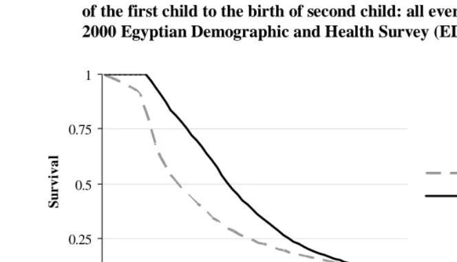
We limit the analysis to the second and third birth intervals as, according to the 2000 Egyptian Demographic and Health Survey (EDHS), few women who approve of family planning think that a newly married couple should use contraception to delay the first birth and only 0.3 percent of currently married women use modern methods of contraception before their first birth (El-Zanaty and Way 2001). More than 50 percent of married women conceive their first child within six months of their first marriage and in just over a year and half 75 percent do so. Among those women in the EDHS who had a first child, 50 percent conceived the second child within a year and half of the birth of the first child, and it took almost two years and a half for 75 percent of them to conceive their second child (Figure 1). Thus the first birth interval is shorter than the second and contraceptive use appears not to play a role in determining its length. Women start using contraception after the first birth.
In section 2 of this paper we present the background to the study and introduce the conceptual framework and the problem of model specification. Section 3 presents the data and considers issues of sample selection. Section 4 presents the method, and section 5 presents the major results.
2. Background and conceptual framework
Bongaarts (1982), using aggregate analysis with countries as units, demonstrated that virtually all important variation in fertility is captured by differences in marriage, breastfeeding, contraception, and induced abortion. He showed that the proportion of the variance explained, using the estimated total fertility rates to predict the actual total fertility rates, was 0.96, a remarkable success for any social scientific model, even one using aggregate data (Rindfuss, Palmore and Bumpass 1987). Moreover, the residual variance in total fertility can plausibly be interpreted as being due to the other proximate determinants which were not included in the aggregate model. In other words, aggregate analyses have found, as they should theoretically, no direct effects of social and economic factors on fertility once the proximate determinants are taken into account.
Figure 1: Kaplan-Meier estimate of the survival function for duration from marriage to the birth of the first child and for duration from the birth of the first child to the birth of second child: all ever married women, 2000 Egyptian Demographic and Health Survey (EDHS)
0 0.25 0.5 0.75 1
1 6 11 16 21 26 31 36 41 46 51 56
Time (months)
Duration since marriage or first birth
S
u
r
vi
va
l
birth of first child
birth of second child
Notes. The Kaplan-Meier estimate for the first birth is based on all ever-married women aged 15-49 included in the 2000 EDHS (15,573 women), whereas the Kaplan-Meier estimate for the birth of second child is based on all the ever-married women who had had a first birth (14,164 women). For estimating the number of months by which 50 percent or 75 percent of women conceived a first or second child we subtract nine months from the number of months by which 50 or 75 percent of women give birth to their first or second child.
Source: 2000 Egyptian Demographic and Health Survey.
So far as data availability is concerned, therefore, the problem arises not just because the information that is collected is not accurate enough, but because some important variables are not collected at all. For example, to study the determinants of birth interval length one would ideally need information about intensity of breastfeeding, and contraceptive use over time (preferably on a month-by-month basis), and about frequency of intercourse. Unfortunately, only rarely does a study designed to look at fertility and family planning in developing countries collect information about breastfeeding and contraceptive use dynamics on a month-by-month basis in longitudinal format, and information on frequency of intercourse is not normally collected at all.
Several authors (Blossfeld and Rohwer 1995, Rindfuss, Palmore and Bumpass 1987) have stressed the fact that the exclusion of important covariates is likely to create mis-specification in the model and provide an incorrect estimate for the shape of the hazard with respect to time. Researchers have tried to cope with this problem of important omitted variables in the model by introducing an error term, and in duration analysis the residual becomes an important part of the model specification. Despite this theoretical rationale for introducing error terms in duration models, in the literature there are still opposing views about the appropriateness of their use (see section 4 for further discussion).
This paper will use data from the 2000 Egyptian Demographic and Health Survey (EDHS). Although DHS data are collected in a cross sectional format, for countries with high contraceptive use recent DHSs have collected retrospective monthly information about contraception, breastfeeding and post-partum amenorrhoea for the five years before the survey date. This study therefore makes use of detailed, month-by-month information on contraception (including data on the method being used in each month), breastfeeding behaviour and post partum amenorrhoea. The study uses a discrete-time hazard model with a gamma-distributed error term to account for unobserved heterogeneity, and discusses the implications for the shape of the hazard and survival functions of the introduction of the error term.
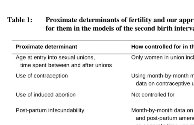
Table 1 lists the proximate determinants of fertility as described by Bongaarts and shows how we control for them in our models. The first group of factors relates to exposure to the risk of sexual intercourse. These are principally the age at marriage and the time spent between marriages and after marriage. In our case, the Egyptian DHS only interviewed ever-married women, and preliminary analysis showed that almost all women were married before they had their first child and remained married until after their third child was born. We therefore restricted the analysis to women who fulfilled these criteria. We use the monthly calendar data to control for contraceptive use and the length of the post-partum infecundable interval. To control for variation in fecundity among women, we include information on the length of time elapsing between marriage and the first birth for women (the vast majority) who were not pregnant when they married. Only 0.3 percent of married women in the EDHS used contraception before the birth of their first child, so the length of the first birth interval is likely to be largely determined by a couple’s fecundity. We do not have data on frequency of intercourse, nor on the duration of viability of ova and sperm. These will, we hope, be captured by the inclusion in the model of an unobserved heterogeneity term.
Finally, there is the question of induced abortion and pregnancies which end in miscarriage. The calendar data do include information about reported pregnancies which are terminated before a live birth. The majority of these were very short (80 per cent being under three months). It is likely that there were additional short pregnancies which ended in miscarriage which were not reported. It is in principle possible to control for these in the model by omitting those months during birth intervals which women spent pregnant in pregnancies which were not carried to term, but in the analysis reported here we chose not to do this. Such pregnancies were relatively few, but we acknowledge that ignoring them is a potential weakness in our analysis. However, it is worth pointing out that by ignoring them we make it more difficult for the calendar data to capture all the proximate determinants of fertility.
Separate consideration is needed of the effect of duration dependence or time since first birth on the risk of conception of the second child. Intuitively the risk of conception will be very low for the first month or two and increase and the decrease thereafter. However, it is not clear exactly what status duration dependence has in this conceptual framework and, whether indeed, its effect still exists after controlling for other socio-economic and biological variables. We will include duration in our analysis in order to see the shape of the baseline hazard after controlling for intermediate variables and unobserved heterogeneity. However, we will bear in mind that duration is also likely to capture both unobservables as well as representing a measure of misspecification (Lancaster 1979).
Table 1: Proximate determinants of fertility and our approach to controlling for them in the models of the second birth interval
Proximate determinant How controlled for in the models
Age at entry into sexual unions, time spent between and after unions
Only women in union included
Use of contraception Using month-by-month method-specific data on contraceptive use
Use of induced abortion Not controlled for
Post-partum infecundability Month-by-month data on breastfeeding and post-partum amenorrhoea introduced as separate time-varying covariates
Spontaneous intra-uterine mortality Not controlled for
Duration of viability of ova and sperm Heterogeneity term
Frequency of sexual intercourse Heterogeneity term
3. Data and sample
The Demographic and Health Survey calendar consists of a matrix of rows and columns. Each row represents a particular month with the first row usually representing January of the fifth calendar year before the survey (for the 2000 EDHS, it represents January 1995). The columns are used to record different types of information for each month. In the 2000 EDHS calendar there are six columns. The first column contains month by month information about births, pregnancies and contraception, the second contains information about the reasons for discontinuation of contraceptive methods, the third about marriages and unions, the fourth about sources of family planning methods, the fifth about post-partum amenorrhoea and the sixth about breastfeeding.
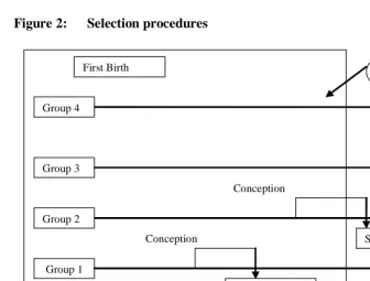
Figure 2: Selection procedures
Conception First Birth
Group 1 Group 2 Group 3
Second birth
Second Birth Observation
Second Birth
5 years calendar Conception
Conception Group 4
Note. In Group 1 there are 1,442 women, in Group 2 there are 242. As we do not experience the second birth for Group 3, we cannot distinguish between women that belong to Groups 3 or 4, though we know that the total number of women for Groups 3 and 4 is 1,215 women.
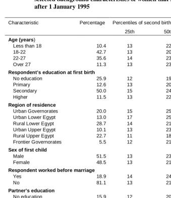
Table 2: Percentage distribution, and 25th, 50th and 75th percentiles of the interval between first birth and conception of second birth by selected background characteristics of women that had a first birth after 1 January 1995
Characteristic Percentage Percentiles of second birth interval (months)
25th 50th 75th
Age (years)
Less than 18 10.4 13 22 32
18-22 42.7 13 20 29
22-27 35.6 14 23 34
Over 27 11.3 13 23 39
Respondent’s education at first birth
No education 25.9 12 19 30
Primary 12.6 13 20 32
Secondary 50.0 15 24 34
Higher 11.5 13 22 32
Region of residence
Urban Governorates 20.0 15 25 39
Urban Lower Egypt 13.0 17 25 36
Rural Lower Egypt 28.7 14 21 30
Urban Upper Egypt 10.1 13 23 36
Rural Upper Egypt 22.7 11 18 28
Frontier Governorates 5.5 12 21 28
Sex of first child
Male 51.5 13 23 34
Female 48.5 13 21 30
Respondent worked before marriage
Yes 18.9 14 24 35
No 81.1 13 21 32
Partner’s education
No education 15.9 12 20 33
Some education 84.1 14 22 32
First child alive
Yes 96.1 14 22 33
No 3.9 5 9 18
Months between marriage and first birth
Less than 19 months 72.0 14 23 32
More than 19 months 28.0 12 20 32
Less than 12 months 51.2 14 24 33
Table 2 Notes. The total number of women is 2,899. Information about educational attainment at the time of the first birth has been derived from the mothers’ age at first birth using the World Higher Education System database (which can be found in the UNESCO website) and assuming that all the women that had some level of education entered schooling at the official entry age for primary education (6 years), and proceeded to further levels of education at the usual ages (14 years for secondary and 19 years for higher education). For example, suppose a mother of age 22 is reported to have ‘higher education’ at the time of the survey. If she had her first child at age 18, then because the entry age for higher education in Egypt is at least 19 years of age, the educational level of this woman when she had her first birth was ‘secondary’. In fact, the educational level at the time of the first birth is different from that reported at the time of the survey for only four women who had higher education level at the time of the survey and secondary education at the time of their first birth. This is probably due to the fact that our sample relates only to women that had their first child after 1 January 1995, leaving a maximum of five years gap between the first birth and survey date. Moreover, most women in Egypt complete their education before they have their first child.
Source. 2000 Egyptian Demographic and Health Survey.
4. Method
We apply a discrete time hazard model of the length of time between first birth and the conception leading to the second live birth. This model specification will allow for a flexible baseline hazard, so there is no need to assume a functional form of the effect of duration. The duration will be broken into k categories (say 0-2 months, 3-5 months, etc…) during each of which the risk of pregnancy is assumed constant for individuals with the same values of the covariates. The degree of flexibility of the baseline hazard will depend on the number of duration dummies in the model.
The discrete time hazard rate is defined as:
Pr[ | , ]
it i i it
h = T =t T ≥t x , (1)
where
x
it is a vector of regressor variables (covariates), some of which can be fixed covariates, and others can be time-varying.T
i is a discrete random variable representing the time at which the end of the spell occurs.We chose to estimate the hazard by applying a discrete time hazard model using a logistic functional form. As Jenkins (1995) suggested, if we reorganize the data in a person-months format, the model likelihood has exactly the same form as that for a standard binary logit regression model. Furthermore this model specification will facilitate the introduction of time-varying covariates in the model. This type of model also allows for censoring in the data.
The hazard rate is defined as follows:
( )
it it(
it)
( )
itit t x h h t x
h =1/{1+exp[−θ −β' ]}⇔log[ /1− ]=θ +β'
, (2)
where )θ(t allows the hazard to vary with time. As has been previously mentioned this specification facilitates the inclusion of time-varying covariates, sincex can include it
both time-varying and fixed covariates. Furthermore the time varying covariates and fixed covariates can have fixed effects as well as time-varying effects.
13-15, 16-18, 19-23, 24-29, 30-36, 37-42, and 43-60 months. Rodriguez (1984) has shown that the estimated effects of covariates are quite insensitive to the choice of partition. We chose the duration categories to be narrow at the beginning of the interval as other studies (Hobcraft and McDonald 1984) have shown that the hazards change quickly at the beginning of the interval, mainly because the effect of lactation changes vary rapidly after birth.
As previously mentioned, in the literature there is diverging opinion about the value of including unobserved heterogeneity in the model. Some authors argue (Jenkins 1997; Lancaster 1979) that failing to account for unobserved heterogeneity in the model will result in an over-estimation of the degree of negative duration dependence in the (true) baseline hazard, and an under-estimate of the degree of positive dependence. This is because women whose unobservable characteristics render them ‘high-risk’, and likely to experience the event of interest have short durations and leave the sample, so that at higher durations the risk set is increasingly composed of women whose unobservable characteristics make them unlikely to experience the event of interest. The result is that failure to account for unobserved heterogeneity will lead the analyst to overestimate the hazard at short durations and underestimate the hazard at longer durations. Moreover, failing to account for unobserved heterogeneity will bias the parameter estimates of regressors as well.
On the other hand, a drawback of accounting for unobserved heterogeneity in the model is that the parameter estimates can be highly sensitive to the assumed parametric form of the error term (Blossfeld and Rohwer 1995). As an example Heckman and Singer (1982) estimated four different unobserved heterogeneity models: one with a normal, one with a log-normal, and one with a gamma distribution of the error term, as well a model with a non-parametric specification of the disturbance. They found that the parameter estimates provided by these models were surprisingly different. In other words, as Blossfeld and Rohwer (1995) suggest, the misspecification of the duration variables caused by neglecting the error term might simply be replaced by misspecification of the parametric distribution of the error term.
which we have not observed, the inclusion of the heterogeneity term allows us to control for their effects.
We present the results both of models without accounting for unobserved heterogeneity and models accounting for unobserved heterogeneity for the purposes of comparison and we discuss the implications of the introduction of unobserved heterogeneity in the model. In the model which accounts for unobserved heterogeneity, the hazard rate is specified:
[
h
it−
h
it]
=
θ
t
+
β
X
it+
ε
i'
)
(
)
1
/(
log
(3)where
ε
i is the unobserved heterogeneity term.The models are estimated using the pgmhaz command in STATA developed by Jenkins (1997). This command estimates, by maximum likelihood, two discrete time grouped duration data proportional hazard models one of which incorporates a gamma mixture distribution to summarize individual unobserved heterogeneity (or ‘frailty’). The two models estimated are (1) the Prentice and Gloeckler (1978) model and (2) the Prentice and Gloeckler (1978) model incorporating a gamma mixture distribution to summarize unobserved individual heterogeneity, as proposed by Meyer (1990). The Prentice-Gloeckler-Meyer models are described by Stewart (1996).
5. Results
In the presentation of the results we shall use two statistics employed by Rodriguez and Hobcraft (1983) in their illustrative analysis of life tables. As originally defined, the
quintum is the proportion of women that have their next birth within five years (60
months). The trimean is a measure of the average birth interval among those women who have their next child within five years (measured by the quintum). The trimean, originally developed by Tukey (1977), contains more information about the shape of the distribution than the median as it includes in its formula the first and third quartiles, thus allowing the detection of asymmetries in the distribution. It is defined as:
(
q1 2q2 q3)
4T = + + ,
pregnancies in a birth interval, the trimean will be higher (slightly) than the median. Rodriguez and Hobcraft (1983) considered the birth interval length and calculated the quintum and trimean for each parity.
In the present study we modify the definition so that it relates to the birth-pregnancy interval (Trussell, Vaughan and Farid, 1988). Hence, the quintum is the estimated proportion becoming pregnant within 51 months and is a direct estimate of the proportion giving birth within five years, and the trimean is a measure of the average birth-pregnancy interval of those women who conceived their second child within 51 months of giving birth to their first. Other measurements that could be calculated to report the dispersion of the data include the spread (or inter-quartile range). The spread, in this case, is the difference between the duration by which 25 per cent of women conceive their second child and the duration by which 75 per cent of women conceive their second child.
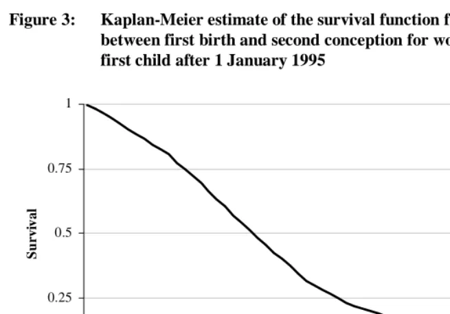
Figure 3 shows the Kaplan-Meier estimate of the survival function from first birth to conception of the second birth for the whole sample. From the Kaplan-Meier estimate the quintum, trimean and spread may be calculated, and these are shown for the whole sample in Table 3, column 1. The quintum is 0.91, which means that 91 per cent of women in our sample that had conceived a first birth conceived the second child within 51 months, with an average first birth-pregnancy interval of almost 20 months. Furthermore 25 per cent of women conceive their second child within a year (11.9 months) and 50 per cent of women in just over a year and a half (19.6 months).
Table 3: Quintum, median, trimean, and spread from Kaplan-Meier estimate and duration-only model (durations in months)
Kaplan-Meier estimate Duration only model
Quintum (Q) 0.91 0.89
1
q
11.9 12.82
q
Median 19.6 21.73
q
27.9 29.9Trimean (T) 19.7 21.5
Figure 3: Kaplan-Meier estimate of the survival function for the interval between first birth and second conception for women that had a first child after 1 January 1995
0 0.25 0.5 0.75 1
1 6 11 16 21 26 31 36 41 46 51 56
Time from first birth (months)
Sur
v
iva
l
Source: 2000 Egyptian Demographic and Health Survey.
5.1 ‘Proximate’ and ‘socio-economic’ models
Consider first Model 1 (Table 4), with only duration as a covariate. Figure 4 shows the shape of the hazard of conception for this model, and demonstrates that the risk of conceiving the second child increases almost monotonically until two years after the birth of the first child, and then decreases. The quintum of this ‘duration-only’ model is 0.89 (89 per cent of women became pregnant within 51 months) and the trimean is 21.5 (Table 3).
Figure 4: Estimated hazard of conception of second birth (duration-only model)
0 0.01 0.02 0.03 0.04 0.05 0.06 0.07 0.08
0 10 20 30 40 50 60
Time from first birth (months)
D
is
cret
e t
im
e h
a
za
rd
Note: In this figure the hazard at duration t months, h(t), is calculated using model 1 in Table 4 using the equation
h(t) = exp(b0 + bt)/[(1 + exp(b0 + bt)], where b0 is the estimated value of the constant (-4.753) and bt is the estimated value of the
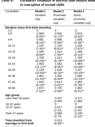
Comparing the ‘proximate’ Model 2 with Model 1 we see that adding the proximate determinants, not surprisingly, dramatically improves the fit of the model. The effect of duration also changes, because the estimated duration effect in Model 1 relates to all women, whereas that in Model 2 relates to a ‘baseline’ group of women who are aged 18-22 years at the time of the first birth and who are not using contraception, not breastfeeding and not amenorrheic. Because breastfeeding, amenorrhoea and contraceptive use vary with duration, the proportion of the risk-set who are in the ‘baseline’ group also varies with duration. The results of Model 2 clearly justify the inclusion in the model of both the information on breastfeeding and amenorrhoea, in that breastfeeding significantly reduces the risk of conception even among non-amenorrheic women. The use of contraception greatly decreases the hazard of conception, with the intra-uterine device (IUD) being slightly more effective in this respect than the pill or other methods.
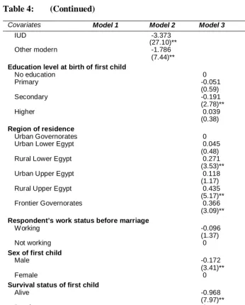
Model 3, the ‘socio-economic’ model, has a much lower explanatory power than Model 2. Although several variables significantly affect the hazard in Model 3, in all but one case the effects are reduced in magnitude in Model 4, which includes both proximate and socio-economic variables. However, Model 4 does mark a significant improvement on the ‘proximate’ model (Model 2). Performing a likelihood-ratio test we have:
(2{Log-Likelihood (full model) - Log-Likelihood (proximate only model)} = 2 x (-6004)-(- 6031)
= 54
with 12 degrees of freedom (p < 0.0005). Model 4 with both socio-economic variables and proximate variables thus performs better than the ‘proximate’ model.
Table 4: Parameter estimates of discrete time hazard models for duration to conception of second child.
Covariates Model 1
Duration only Model 2 Proximate variables only Model 3 Socio-economic variables only Model 4
Both proximate and socio-economic variables
Duration since first birth (months)
1-2 0 0 0 0
3-5 0.908 0.935 0.919 0.943
(5.55)** (5.17)** (5.62)** (5.21)**
6-9 0.981 0.998 1.006 1.006
(6.14)** (5.56)** (6.28)** (5.60)**
10-12 1.220 1.218 1.258 1.223
(7.45)** (6.61)** (7.67)** (6.62)**
13-15 1.440 1.414 1.486 1.420
(8.84)** (7.64)** (9.11)** (7.65)**
16-18 1.708 1.612 1.769 1.613
(10.55)** (8.70)** (10.89)** (8.67)**
19-23 1.903 1.582 1.984 1.580
(12.17)** (8.65)** (12.66)** (8.57)**
24-29 2.139 1.529 2.247 1.535
(13.56)** (8.14)** (14.20)** (8.07)**
30-36 1.961 1.202 2.086 1.226
(11.54)** (6.04)** (12.23)** (6.08)**
37-42 1.843 0.914 1.983 0.943
(9.12)** (4.01)** (9.76)** (4.09)**
43-60 1.674 0.725 1.863 0.771
(7.51)** (2.94)** (8.31)** (3.09)** Age group
Less than 18 years -0.207 -0.171 -0.167
(2.40)* (1.98)* (1.90)
18-22 years 0 0 0
22-27 years 0.072 -0.085 0.054
(1.23) (1.42) (0.87)
Over 27 years -0.068 -0.195 -0.125
(0.73) (2.12)* (1.25)
Time (months) from -0.013 -0.012
marriage to first birth (8.30)** (7.67)**
Amenorrheic
Yes -1.226 -1.237
(11.66)** (11.72)**
No 0 0
Breastfeeding
Yes -0.477 -0.504
(7.15)** (7.10)**
No 0 0
Type of contraceptive method being used
Table 4: (Continued)
Covariates Model 1 Model 2 Model 3 Model 4
IUD -3.373 -3.427
(27.10)** (27.32)**
Other modern -1.786 -1.861
(7.44)** (7.71)**
Education level at birth of first child
No education 0 0
Primary -0.051 0.036
(0.59) (0.40)
Secondary -0.191 -0.080
(2.78)** (1.12)
Higher 0.039 0.366
(0.38) (3.36)** Region of residence
Urban Governorates 0 0
Urban Lower Egypt 0.045 0.115
(0.48) (1.19)
Rural Lower Egypt 0.271 0.170
(3.53)** (2.13)*
Urban Upper Egypt 0.118 -0.008
(1.17) (0.08)
Rural Upper Egypt 0.435 0.003
(5.17)** (0.03)
Frontier Governorates 0.366 0.107
(3.09)** (0.88) Respondent’s work status before marriage
Working -0.096 -0.165
(1.37) (2.26)*
Not working 0 0
Sex of first child
Male -0.172 -0.105
(3.41)** (2.02)*
Female 0 0
Survival status of first child
Alive -0.968 0.184
(7.97)** (1.39)
Dead 0 0
Partner’s education
No education 0 0
Some education 0.128 0.258
(1.71) (3.33)**
Constant -4.753 -3.061 -3.922 -3.422
(33.13)** (17.00)** (19.11)** (14.83)** Pseudo R squared 0.0318 0.1791 0.0415 0.1827
Observations 2899 2899 2899 2899
Log-Likelihood -7147.0 -6031.0 -7075.6 -6004.3
Figure 5 shows the estimated shape of the hazard for four types of women: (1) a woman that did not breastfeed, who was never subject to post-partum amenorrhoea and who did not use contraception over the study period; (2) a woman who used the pill but did not breastfeed and was never subject to post-partum amenorrhoea; (3) a woman who used the IUD, did not breastfeed and who was never subject to post-partum amenorrhoea; and (4) a woman who used ‘other modern methods’, who did not breastfeed and who was never subject to post-partum amenorrhoea. Despite the fact that the shapes of the hazards displayed below refer to hypothetical women, Figure 5 helps to reveal the effectiveness of different types of contraceptive method. The IUD is the most effective method of contraception, whereas the pill is a less effective method.
Figure 5: Estimated hazard of conception of second birth for selected women
0 0.02 0.04 0.06 0.08 0.1 0.12 0.14
0 10 20 30 40 50 60
Ti me from fi rs t bi rth (m on ths )
D
is
cre
te
t
im
e
h
a
za
rd
No Breastfeeding, no contraceptive use, no amenorrhea
IUD
Pill
Other modern methods
Note: In this figure the hazard at duration t months, h(t), is calculated using Model 4 in Table 4 using the equation
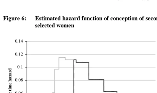
Figures 6 and 7 show the hazard and survivor functions of four more ‘realistic’ groups of women. All these groups of women were both breastfeeding and amenorrheic for the first four months after the birth of the first child. After this the amenorrhoea ceased, but they kept on breastfeeding until month 13 after the first child was born. The first group did not use contraception at all during the observation period. The second group used the IUD for 18 months after the period of amenorrhoea ended (they were both breastfeeding and using contraception for nine months, after which they continued to use the IUD for another 9 months). The third and fourth groups are like the second group, except that they used the pill and ‘other modern methods’ respectively instead of the IUD. Calculations of the quintum and trimean of fertility for the groups of women in Figures 6 and 7 show that there is a difference of two months in the average birth-conception interval between women using IUDs and women using the pill or ‘other modern methods’ of contraception, suggesting differences in contraceptive failure rates between women using the IUD and women using the pill or ‘other modern methods’. The IUD is the most reliable method of contraception in Egypt.
Figure 6: Estimated hazard function of conception of second birth for
selected women
0 0.02 0.04 0.06 0.08 0.1 0.12 0.14
0 10 20 30 40 50 60
Time from first birth (months)
D
is
cr
et
e t
im
e
h
a
za
rd
No contraception
IUD
Pill
Other M odern M ethods
Figure 7: Estimated survival function of conception of second birth for
selected women
0 0.2 0.4 0.6 0.8 1
0 10 20 30 40 50 60
Time from first birth (months)
Su
rv
iv
a
l
No contraception
IUD
Pill
Other M odern M ethods
Note. See text for detailed description of the characteristics of women in each category. The survival function for a particular group of
women at duration t, S(t), is derived from the relevant hazard function in Figure 6 using the equation
0
( ) exp ( )
t
S t = − h s ds
∫ ,
where h(s) is the appropriate hazard in Figure 6.
partner of the respondent has some level of education the relative risk of conception is 29 per cent higher, resulting in a shorter birth interval.
One possible explanation of the continued significance of some social, economic and cultural variables in Model 4 is that, although the framework of Bongaarts (1982) still holds in general, including the socio-economic variables improves our measurement of the impact of intermediate variables. For example, if the first child is a boy, one would expect more contraceptive use because of a reduced need to have a second child quickly compared to the situation when the first child is a girl. However the ‘sex-of-first-child’ effect is still significant after accounting for contraceptive use and duration of breastfeeding. This might be because, for example, boys are breastfed more intensely than girls, or that contraception is used more carefully after a boy than a girl. Furthermore, higher educated women appear to have a higher risk of conception compared to women with no education. This could be explained by the fact that higher educated women are those who rely more on traditional methods, such as periodic abstinence (Esseghairi 2003).
The gradual erosion of the contraceptive effect of breastfeeding as the first child grows up also explains why no multicollinearity problem exists with the introduction in the model of both breastfeeding information and the period of post-partum amenorrhoea. The results confirmed previous findings on the effect of breastfeeding net of amenorrhoea on fertility (Jain et al. 1970) and show the importance of including both information on breastfeeding and post-partum amenorrhoea in model specification in birth interval analysis. In addition, no multicollinearity problem appears also to exist between respondent’s and husband’s educational level, and between respondent’s work status before marriage and respondent’s level of education.
5.2 Effect of length of first interval and contraception on the second birth interval
We estimated three additional models to show the changes in the effect of other covariates on the hazard of conception of the second birth after having excluded the contraception variables, and to assess if the effect of the length of the interval between marriage and birth (the first birth interval) is linear and if this effect changes with the exclusion of contraceptive use variables. Model 5 is the same as Model 4 but without the contraceptive use variables. Model 6 is a variation of Model 4 in which the length of the first birth interval is allowed to have a non-linear (quadratic) effect on the hazard. Model 7 is, in effect, a combination of Models 5 and 6, in that it both excludes the contraceptive use variables and allows the length of the first birth interval to have a quadratic effect.
include contraceptive use variables (see Model 7). If we include contraceptive use variables in the model, the effect of the first birth interval length on the second birth interval is linear, as illustrated by the non-significant coefficient for the square of length of birth interval in Model 6. This result might be interpreted by suggesting that women who experience a short first birth interval consider themselves to be especially fecund and therefore are especially careful in their use of contraception to delay the second birth. Conversely, women who found it difficult to conceive their first child (that is, they had a long first birth interval), might rely on their low fecundity to produce an acceptably long second birth interval.
Comparing Models 4 and 5, there are changes in the effect of several socio-economic covariates when contraceptive use is excluded. Without the contraceptive use variables, the effect of having a secondary education is significant, whereas the effect of having higher education becomes insignificant. The effect of being resident in rural Upper Egypt and Frontier Governorates and the survival status of first child are significant when contraceptive use is excluded, but not when it is included. The opposite is true of husband’s education.
5.3 Unobserved heterogeneity
We re-estimated Model 4 (the combined ‘socio-economic’ and ‘proximate’ model) incorporating the term for gamma-distributed unobserved heterogeneity. The results (Table 6) show that the unobserved heterogeneity parameter is significant suggesting that individual-level unobserved heterogeneity should be part of the model. The parameter estimates on the social and economic covariates change very little when the unobserved heterogeneity term is added, suggesting that there is little correlation between the unobservables and the socio-economic covariates included in the model. It therefore seems plausible to conclude that the heterogeneity term is largely picking up unobserved variations in fecundity due, for example, to physiological factors or coital frequency.
economic variables except husband’s education lose their significance, whereas proximate variables such as amenorrhoea and contraceptive use become more significant.
In Table 6 (columns 3 and 4) are also shown the results for a ‘combined’ model of the third birth interval with and without unobserved heterogeneity. The results for the third birth interval show that all the variation in birth interval length is captured by the proximate determinants. The effects of work and education which were found to be significant for the second birth interval are not significant here. In order to test formally for differences between the second birth interval and third birth interval model a likelihood ratio test has been performed. The log-likelihood of a model for the data for the second and third intervals pooled together and the sum of log-likelihoods of the separate models for the second and the third interval have been used. This procedure can only be approximate for several reasons. First, when performing the likelihood ratio test only a subset of the parameters included in the models in Table 6 can be considered. In particular, survival status of the first child is less relevant for the third birth interval as for the second birth interval, and the effect of the variable ‘sex of the first child’ cannot be directly compared across both intervals as the option of a mixed pair is possible in the case of the third birth interval. Moreover, pooling together the women who had a second birth and a third birth implies that the observations will be dependent of each other.
With these caveats, the results suggest that the two models are significantly different. The likelihood of the pooled model is 7252.67 and the sum of the log-likelihoods for the models of the second and third birth intervals taken separately is 7219.17. A likelihood ratio test performed using twice the difference between the log-likelihoods gives a value of 67 with 29 degrees of freedom (p = 0.0005). Part of the difference between the models is due to the fact that the women selected for the third birth interval analysis are only those who had a second birth in the five years prior the survey date (as opposed to women who had a first birth within this window in the analysis for the second birth interval) and for this reason not only tend to belong to an older cohort but are also a ‘more’ selected group of women as they already had their second birth.
Table 5: Parameter estimates for discrete time hazard models for duration to conception of second child
Covariate Model 4 Model 5
Without contraceptive use variables Model 6 With non-linear effect of first birth interval
Model 7
With non-linear effect of first birth interval and without contraceptive use variables
Duration since first birth(months)
1-2 0 0 0 0
3-5 0.943 0.779 0.942 0.775
(5.21)** (4.34)** (5.20)** (4.32)**
6-9 1.006 0.785 1.005 0.779
(5.60)** (4.40)** (5.59)** (4.37)**
10-12 1.223 0.987 1.221 0.979
(6.62)** (5.39)** (6.61)** (5.35)**
13-15 1.420 1.162 1.418 1.154
(7.65)** (6.32)** (7.64)** (6.28)**
16-18 1.613 1.390 1.612 1.385
(8.67)** (7.57)** (8.67)** (7.54)**
19-23 1.580 1.379 1.578 1.373
(8.57)** (7.58)** (8.56)** (7.55)**
24-29 1.535 1.452 1.534 1.447
(8.07)** (7.76)** (8.07)** (7.73)**
30-36 1.226 1.252 1.225 1.243
(6.08)** (6.30)** (6.07)** (6.26)**
37-42 0.943 1.155 0.941 1.141
(4.09)** (5.09)** (4.08)** (5.03)**
43-60 0.771 1.039 0.770 1.030
(3.09)** (4.22)** (3.09)** (4.18)** Age group
Less than 18 years -0.167 -0.204 -0.164 -0.188 (1.90) (2.35)* (1.86) (2.16)*
18-22 years 0 0 0 0
22-27 years 0.054 -0.061 0.052 -0.074 (0.87) (1.01) (0.83) (1.23) Over 27 years -0.125 -0.077 -0.122 -0.054 (1.25) (0.80) (1.21) (0.56) Educational level at birth of first child
No education 0 0 0 0
Primary 0.036 -0.069 0.039 -0.058
(0.40) (0.79) (0.44) (0.67)
Secondary -0.080 -0.239 -0.077 -0.224
(1.12) (3.44)** (1.08) (3.21)**
Higher 0.366 -0.003 0.370 0.016
(3.36)** (0.03) (3.39)** (0.15)
Region of residence
Urban Governorates 0 0 0 0
Table 5: (Continued)
Covariate Model 4 Model 5 Model 6 Model 7
Rural Upper Egypt 0.003 0.532 0.000 0.512 (0.03) (6.28)** (0.00) (6.03)** Frontier Governorates 0.107 0.428 0.108 0.436
(0.88) (3.59)** (0.89) (3.66)** Respondent’s work status before marriage
Working -0.165 -0.162 -0.164 -0.155
(2.26)* (2.31)* (2.25)* (2.20)*
Not working 0 0 0 0
Sex of first child
Male -0.105 -0.165 -0.105 -0.165
(2.02)* (3.25)** (2.03)* (3.25)**
Female 0 0 0 0
Survival status of first child
Alive 0.184 -0.488 0.184 -0.485
(1.39) (3.72)** (1.39) (3.70)**
Dead 0 0 0 0
Partner’s education
No education 0 0 0 0
0.258 0.079 0.258 0.090 Some education ( 3.33)** (1.04) (3.33)** (1.19) Amenorrheic
Yes -1.237 -0.571 -1.237 -0.582
(11.72)** (5.44)** (11.73)** (5.56)**
No 0 0 0 0
Breastfeeding
Yes -0.504 -0.645 -0.504 -0.647
(7.10)** (9.52)** (7.11)** (9.54)**
No 0 0 0 0
Type of contraceptive method being used
None or traditional 0 0
Pill -2.190 -2.188
(14.80)** (14.78)**
IUD -3.427 -3.424
(27.32)** (27.27)**
Other modern methods -1.861 -1.862
(7.71)** (7.72)**
Time from marriage to -0.012 -0.004 -0.010 0.007 first birth (months) (7.67)** (3.30)** (2.88)** (2.21)*
Time from marriage -0.002 -0.009
to first birth (0.74) (3.39)**
squared / 100
Constant -3.422 -3.417 -3.452 -3.587
(14.83)** (15.00)** (14.74)** (15.45)**
Pseudo R-square 0.1827 0.0520 0.1828 0.0531
Observations 2899 2899 2899 2899
Log-Likelihood -6004.3 -6965.0 -6004.0 -6957.0
Table 6: Discrete-time hazard models of time to conception of second and third births for models with and without accounting for unobserved heterogeneity
Covariate Second birth
without unobserved heterogeneity Second birth with gamma-distributed heterogeneity Third birth without unobserved heterogeneity
Third birth with gamma-distributed heterogeneity
Duration since previous birth (months)
1-2 0 0 0 0
3-5 0.943 1.057 0.756 1.074
(5.21)** (5.60)** (2.01)** (2.51)**
6-9 1.006 1.291 1.417 1.936
(5.60)** (6.85)** (3.99)** (4.70)**
10-12 1.223 1.642 1.060 1.851
(6.62)** (8.43)** (2.73)** (4.13)**
13-15 1.420 1.965 1.551 2.484
(7.65)** (9.92)** (4.10)** (5.56)**
16-18 1.613 2.260 1.865 3.005
(8.67)** (11.26)** (4.93)** (6.51)**
19-23 1.580 2.303 1.660 3.046
(8.57)** (11.24)** (4.34)** (6.27)**
24-29 1.535 2.401 1.557 3.133
(8.07)** (11.06)** (3.79)** (5.95)**
30-36 1.226 2.397 1.731 3.409
(6.08)** (10.06)** (4.00)** (6.04)**
37-42 0.943 2.318 1.336 3.303
(4.09)** (8.38)** (2.08)** (4.10)**
43-60 0.771 2.438 0.617 3.313
(3.09)** (7.69)** (0.57) (2.40)* Age group
Less than 18 years -0.167 -0.209 0.110 0.152 (1.90)* (1.60) (0.59) (0.53)
18-22 years 0 0 0 0
22-27 years 0.054 0.079 0.135 0.468
(0.87) (0.87) (0.90) (2.10)*
Over 27 years -0.125 0.026 -0.441 0.023
(1.25) (0.18) (1.65)* (0.06) Educational level at birth of first child
No education 0 0 0 0
Primary 0.036 0.018 -0.200 -0.306
(0.40) (0.14) (1.02) (1.08)
Secondary -0.080 -0.157 0.018 0.015
(1.12) (1.51) (0.11) (0.06)
Higher 0.366 0.255 0.148 0.068
(3.36)** (1.63) (0.48) (0.17) Region of residence
Urban Governorates 0 0 0 0 Urban Lower Egypt 0.115 0.111 0.253 -0.180
Table 6: (Continued)
Rural Lower Egypt 0.170 0.185 0.046 -0.343 (2.13)* (1.60) (0.20) (1.10) Urban Upper Egypt -0.008 0.185 -0.036 -0.246 (0.08) (1.21) (0.14) (0.65) Rural Upper Egypt 0.003 0.117 0.126 -0.139 (0.03) (0.92) (0.56) (0.45) Frontier Governorates 0.107 0.131 -0.054 -0.075 (0.88) (0.73) (0.19) (0.18) Respondent’s work status before marriage
Working -0.165 -0.174 0.114 -0.048
(2.26)* (1.62) (0.60) (0.18)
Not working 0 0
Sex of first (two) child(ren)
Male -0.105 -0.105 0.219 0.088
(2.02)* (1.39) (1.24) (0.35)
Female 0 0 0 0
Mixed pair n.a n.a. 0.065 0.057
(0.43) (0.26) Survival status of first child
Alive 0.184 0.068 -0.380 -0.688
(1.39) (0.34) (2.41)* (2.79)**
Dead 0 0 0 0
Partner’s education
No education 0 0 0 0
Some education 0.258 0.254 -0.093 -0.141 (3.33)** (2.24)* (0.57) (0.57) -0.012 -0.014 -0.001 -0.001 Time from marriage to
first birth (7.67)** (6.81)** (0.17) (0.23)
Amenorrheic
Yes -1.237 -1.483 -1.321 -1.607
(11.72)** (12.96)** (6.34)** (6.85)**
No 0 0 0 0
Breastfeeding
Yes -0.504 -0.575 -0.678 -0.778
(7.10)** (6.62)** (4.31)** (3.89)**
No 0 0 0 0
Type of contraceptive method being used
None or traditional 0 0 0 0
Pill -2.190 -2.621 -2.496 -3.234
(14.80)** (16.03)** (7.87)** (8.58)**
IUD -3.427 -4.064 -3.400 -4.296
(27.32)** (29.55)** (13.93)** (13.67)** Other modern methods -1.861 -2.119 -4.365 -5.199
(7.71)** (7.59)** (4.34)** (4.95)**
Constant -3.422 -3.166 -3.680 -2.921
(14.83)** (10.70)** (8.03)** (4.73)**
Gamma variance 0.939 0.342
(11.16)** (1.69)
Log-Likelihood -6004.1 -5859.9 -1207.9 -1172.1
Notes. The models for the third birth interval include 1,270 women who had a second child after 1 January 1995 of which 309 conceived their third child before the survey date. Absolute value of z-statistics in parentheses.
Figure 8: Discrete time hazard with and without unobserved heterogeneity for women in the reference category
0 0.05 0.1 0.15 0.2 0.25 0.3
0 10 20 30 40 50 60
Ti me from fi rst birth (m onths )
Di
sc
r
et
e t
im
e h
a
za
rd No unobserved
heterogeneity
Unobserved heterogeneity
6. Conclusion
Using Bongaarts’s (1982) framework of the proximate determinants of fertility, which shows that all important variation in fertility is captured by variation in the proximate determinants, this paper assesses the reliability of the Demographic and Health Survey (DHS) calendar data. Most previous assessments of the reliability of those data have used aggregate techniques. However, the question we pose here is not whether individual level responses of calendar data are reliable or not, but rather: are the calendar data good enough to capture all the ‘measurable variation’ in fertility?
Our results show that once the calendar data on the proximate determinants are fully incorporated into a model, social, economic and cultural factors become insignificant. This is particularly so when an unobserved heterogeneity term is included in the model to capture variation in those proximate determinants which are hard to measure directly. Hence, the paper shows that calendar data provides important information to enable demographers potentially to identify the pathways by which social and economic factors influence fertility.
The results of this analysis demonstrate the importance of introducing detailed month-by-month information on contraception in birth interval analysis. They also show that we should not only include in the analysis the period of breastfeeding but also the period of post-partum amenorrhoea. The results suggest that the inclusion in the model of socio-economic variables can improve our measurement of the impact of biological variables in a model which does not control for unobserved heterogeneity. However, when unobserved characteristics are controlled for by incorporating a heterogeneity term, the direct impact of socio-economic variables on the hazard of conception becomes very small.
they allow the use of more exposure states than conventional retrospective survey data (see Hobcraft and Little, 1984: 23).
Despite the fact that the analysis reported in this paper was not designed to study contraceptive failure rates, it can help to provide some insight into contraceptive failure in Egypt. The results show a degree of failure of contraceptive use. The level of contraceptive failure varies by method, though a degree of failure is present in every method of contraceptive use. It seems that in Egypt the IUD is less prone to failure than the pill or other modern methods. This suggests that policy makers should not only look to increase uptake of contraceptive methods but improve family planning counselling, as contraceptive methods have still a degree of failure.
7. Acknowledgments
References
Blossfeld, H.-P.and G. Rohwer. 1995. Techniques of event history modelling: new
approaches to casual analysis. Mahwah, New Jersey: Lawrence Erlbaum
Associates.
Bongaarts, J. 1978. ‘A framework for analysing the proximate determinants of fertility.’
Population and Development Review 4:105-132.
Bongaarts, J. 1982. ‘The fertility-inhibiting effects of the intermediate fertility variables.’
Studies in Family Planning 13:178-189.
Bumpass, L.L., R.R. Rindfuss, and P. James. 1986. ‘Determinants of Korean birth intervals: the confrontation of theory and data.’ Population Studies 40:403-423. Curtis, S.L. 1997. ‘Using calendar data to study contraceptive use.’ Paper presented at
the IUSSP/EVALUATION Project Seminar on Methods for Evaluating Family Planning Program Impact, May 14-16 1997, Costa Rica.
Curtis, S.L. and A.K. Blanc. 1997. Determinants of contraceptive failure, switching and discontinuation: an analysis of DHS contraceptive histories. Analytical Report no. 6. Calverton, MD: Macro International.
Davis, K.and J. Blake. 1956. ‘Social structure and fertility: an analytic framework.’
Economic Development and Cultural Change 4:211-235.
El-Zanaty, F. and A. Way. 2001. Egypt Demographic and Health Survey 2000.
Esseghairi, K. 2003. ‘Sustaining fertility control in Tunisia while addressing emerging reproductive health needs: a comparison with Algeria.’ Unpublished MPhil thesis, Department of Social Statistics, University of Southampton.
Gertler, P.J. and J.W. Molyneaux. 1994. ‘How economic development and family planning programs combined to reduce Indonesian fertility.’ Demography 31:33-63.
Heckman, J.J. and B. Singer. 1982. ‘The identification problem in econometric models for duration data.’ In: Hildenbrand, W. ed., Advances in econometrics. Cambridge: Cambridge University Press, 39-77.
Hobcraft, J. and R.J.A. Little. 1984. ‘Fertility exposure analysis: a new method for assessing the contribution of proximate determinants to fertility differentials.’
Hobcraft, J. and J. Mc Donald. 1984. ‘Birth intervals. World Fertility Survey Comparative Studies no. 28. Voorburg, Netherlands: International Statistical Institute.
Jain, A., A. Hermalin and T.-H. Sun. 1979. ‘Lactation and natural fertility.’ In: Leridon, H. and Menken, J.
Jenkins, S.P. 1995. ‘Easy estimation methods for discrete-time duration models.’ Oxford
Bulletin of Economics and Statistics 57:129-138.
Jenkins, S.P. 1997. ‘Estimation of discrete time (grouped duration data) proportional hazards models: pgmhaz.’ in Mimeo: ESRC Research Centre on Micro-Social Change, University of Essex.
Kallan, J. and J.R. Udry. 1986. ‘The determinants of effective fecundity based on the first birth interval.’ Demography 23:53-66.
Lancaster, T. 1979. ‘Econometric methods for the duration of unemployment.’
Econometrica 47:939-956.
Leone, T. 2002. ‘Fertility and union dynamics in Brazil.’ Unpublished PhD thesis, Department of Social Statistics, University of Southampton.
Magnani, R.J., N. Rutenberg, and H.G. McCann. 1996. ‘Detecting induced abortions from reports of pregnancy terminations in DHS calendar data.’ Studies in Family
Planning 27:36-43.
McDonald, J. and P.J. Egger. 1990. ‘Discrete-time survival model for the analysis of birth intervals.’ Paper presented at the Annual Meeting of the Population Association of America. Toronto, Canada.
McNeilly, A.S. 1993. ‘Breastfeeding and fertility’. In: Gray, R.H., Leridon, H. and Spira, A., eds. Biomedical and demographic determinants of reproduction. Oxford: Clarendon Press, 391-412.
Meyer, B.M. 1990. ‘Unemployment insurance and unemployment spells.’ Econometrica 58:757-782.
Palloni, A. 1984. ‘Assessing the effects of intermediate variables on birth interval-specific measure of fertility.’ Population Index 50:623-657.
Rindfuss, R.R., J.A. Palmore, and L.L. Bumpass. 1987. ‘Analyzing birth intervals: implications for demographic theory and data collection.’ Sociological Forum 4:811-828.
Rodriguez, G. 1984. The analysis of birth intervals using proportional hazard models. World Fertility Survey Technical Report no. 2314. Voorburg, Netherlands: International Statistical Institute.
Rodriguez, G. and J. Hobcraft. 1983. Illustrative analysis: life table analysis of birth intervals in Colombia. World Fertility Survey Scientific Report no. 16. Voorburg, Netherlands: International Statistical Institute.
Steele, F. and S.L. Curtis. 2003. ‘Appropriate methods for analyzing the effect of method choice on contraceptive discontinuation.’ Demography 40:1-22.
Steele, F., S.L. Curtis and M. Choe. 1999. ‘The impact of family planning service provision on contraceptive-use dynamics in Morocco.’ Studies in Family Planning 30:28-42.
Stewart, M.B. 1996 ‘Heterogeneity specification in unemployment duration models.’ Mimeo: Department of Economics, University of Warwick.
Strickler, J.A., R.J. Magnani, H.G. McCann, L.F. Brown and J.C. Rice. 1997. ‘The reliability of reporting of contraceptive behaviour in DHS calendar data: evidence from Morocco.’ Studies in Family Planning 28: 44-53.
Trussell, J., L.G. Martin, R. Feldman, J.P. Palmore, M. Concepcion and D.N.L.B.D.A. Bakar. 1985. ‘Determinants of birth-interval length in the Philippines, Malaysia and Indonesia: a hazard-model analysis.’ Demography 22:145-168.
Trussell, J., B. Vaughan and S. Farid. 1988. ‘Determinants of birth interval length.’ In: Hallouda, A.M., Farid, S. and Cochrane, S.H. eds, Egypt demographic responses
to modernization. Cairo: Central Agency for Public Mobilization and Statistics.
Tukey, J.W. 1977. Exploratory data analysis. New York: Addison-Wesley.