Bifurcation and chaos of an SIS model with logistic term

Adv. Fixed Point Theory, 9 (2019), No. 2, 99-110 https://doi.org/10.28919/afpt/4000

ISSN: 1927-6303

BIFURCATION AND CHAOS OF AN SIS MODEL WITH LOGISTIC TERM

NING CUI1,∗, XIAOCHUN ZHONG2, JUNHONG LI1,3

1_{Department of Mathematics and Sciences, Hebei Institute of Architecture and Civil Engineering, Zhangjiakou,}

Hebei, 075000, China

2_{Office of Academic Affairs, Hebei Institute of Architecture and Civil Engineering, Zhangjiakou, Hebei, 075000,}

China

3_{School of Mathematics and Statistics, Beijing Institute of Technology, Beijing, 100081, China}

Copyright c2019 the authors. This is an open access article distributed under the Creative Commons Attribution License, which permits

unrestricted use, distribution, and reproduction in any medium, provided the original work is properly cited.

Abstract.This paper presents a discrete-time SIS epidemic model with Logistic term. The transcritical bifurcation, flip bifurcation and Hopf bifurcation are investigated. The results show that the epidemic system with Logistic

growth of susceptible population has rich dynamic behaviors, including period-6, 7, 8, 10, 11-orbits and chaotic

phenomena.

Keywords:SIS model; logistic term; bifurcation; chaotic attractor.

2010 AMS Subject Classification:37F99, 65E05.

1.

INTRODUCTION

Studies of epidemic models that incorporate the disease causing death and variation in total

population have become one of the important areas in the mathematical theory of epidemiology.

In the theory of epidemics, there are two kinds of mathematical models: the continuous-time

models described by differential equations and the discrete-time models described by difference

∗_{Corresponding author}

E-mail address: [email protected]

Received January 18, 2019

equations. The continuous-time epidemic models have been widely studied in many literatures

[1-6]. Recently, discrete-time epidemic models have been used to study [7-14]. The

advan-tages of a discrete-time approach are multiple. Firstly, difference models are more realistic than

differential ones since the epidemic statistics are compiled from given time intervals and are

discontinuous. Secondly, the discrete-time models can provide natural simulators for the

con-tinuous cases. One can thus not only study the behaviors of the concon-tinuous-time model with

good accuracy, but also assess the effect of lager time steps. Finally, the use of discrete-time

models makes it possible to use the entire arsenal of methods recently developed for the study

of mappings and lattice equations, either from the integrability and/or chaos points of view.

On the other hand, simple models, by their own nature, cannot incorporate many of the

com-plex biological factors. However, they often provide useful insights to help our understanding

of complex process. For such reasons, assume only susceptible population are capable of

re-producing with logistic equation [15-18], we firstly focus on the SIS model with Logistic term

(1)

 

 dS

dt =rS(1− N

K)−βSI+γI, dI

dt =βSI−dI−γI,

Where S, I are denoted the susceptible and infected, respectively. N =S+I is the total

population. All these of course are functions of time. r is the intrinsic birth rate. K, β are the

carrying capacity and the infection rate respectively. γ ≥0 is the recovery rate. d is the death

rate ofI.

Let

S= d+γ

β ,I=

(d+γ)K

r+βK I1,τ= (d+γ)t.

We obtain the following system analogous to (1)

(2)

 

 dS1

dτ =m1S1−m2S

2

1−S1I1+m3I1, dI

dτ =S1I1−I1,

where

In this paper, we apply the Euler scheme to discrete the SIS epidemic model and investigate

the dynamical behaviors in detail by using bifurcation theory and center manifold theory

[19-21]. It is verified that there are phenomena of the transcritical bifurcation, flip bifurcation, Hopf

bifurcation types and chaos.

This paper is organized as follows. In Section 2, we give sufficient conditions of existence

for transcritical bifurcation, flip bifurcation and Hopf bifurcation. In Section 3, a series of

numerical simulations show that there are bifurcation and chaos in the discrete-time epidemic

model. Finally, we give remarks to conclude this paper in Section 4.

2.

DYNAMIC ANALYSIS

2.1.

Existence of fixed points. Applying the Euler scheme to (2), we obtain the discrete

sys-tem

(3)

 



S_1n+1= (m₁+1)S_1n−m₂S_1n2 −S_1nI_1n+m₃I_1n, I_1n+1=S_1nI_1n.

The fixed points of (3) satisfy the following equations

(4)

 



m1S1−m2S2₁−S1I1+m3I1=0,

I₁−S₁I₁=0.

By the analysis of roots for Eq. (4), we obtain the following theorem

Theorem 1. (i). (3) has three fixed pointsP₀(0,0), P₁(m1

m2,0), andP2(1,

m1−m2

1−m3 ), when m1> m₂. (ii) Ifm₁≤m₂, (3) has two fixed pointsP₀(0,0),P₁(m1

m2,0).

The Jacobian matrix of the system (3) at fixed pointP(S_1n,I_1n)takes the form

(5) J(P) =





1+m₁−2m₂S_1n−I_1n m₃−S_1n

I_1n S_1n





2.2.

Bifurcations. It is easy to see that the fixed pointP₀(0,0)is a saddle. In the following, we focus on investigating the bifurcations ofP₁,P₂.

Theorem 2. Ifm₂=m₁andm₁6=2, (3) undergoes a transcritical bifurcation atP₁.

Proof. The Jacobian matrixJ(P₁)has eigenvalues λ1=1−m1, λ2=1 whenm2=m1, and

m₁6=2 implies|λ1| 6=1.

x_n=S_1n−m1

m2,yn=I1n,cn=m1−m2,

(3) becomes (6)         

x_n+1= (1−m₂)x_n+ (m₃−1)y_n−x_n(m₂x_n+c_n+y_n)−cnyn

m2 ,

y_n+1=yn+c_mny₂n +xnyn,

c_n+1=c_n.

By the following transformation

     x_n y_n c_n      =     

1 1 0

1 m2

m3−1 0

0 0 1

          φn ψn σn      (6) becomes     

φn+1

ψn+1

σn+1      =     

1−m₂ 0 0

0 1 0

0 0 1

          φn ψn σn      +     

f₁(φn,ψn,σn)

f2(φn,ψn,σn)

0      where

f₁(φn,ψn,σn) =−m2φn2−(

(2m2m3+m3−m2−1)ψn

m3−1 +σn)φn−

m2m3+m3−1

m3−1 ψ

2

n−m2m3

+m3−1

m2(m3−1) ψn, f2(φn,ψn,σn) =ψ_n2+ψ_mnσn

2 +φnψn.

Then, we can consider

φn=g(ψn,σn) =ε1ψ_n2+ε2ψnσn+ε3σ_n2+o((|ψn|+|σn|)3),

which must satisfy

g(ψn+f2(g(ψn,σn),ψn,σn),σn+1) = (1−m2)g(ψn,σn) + f1(g(ψn,σn),ψn,σn).

Thus, we have

ε1= m_m2m₂₋3+_mm_2m3−₃1,ε2=m_m2m23+m3−1 2−m

2 2m3

,ε3=0.

And (6) is restricted to the center manifold, which is given by

f :ψn+1=ψn+ψn2+

ψnσn

m2 +

m2m3+m3−1

m2−m2m3 ψ

3 n+

m2m3+m3−1

m2 2−m

2 2m3

ψ_n2σn+o((|ψn|+|σn|)4).

Since

f(0,σn) =0, _{∂ ψ}∂f

_(0,0) =1, ∂

2_f

∂ ψ2

_(0,0) =2, ∂

2_f

∂ ψ ∂ σ

_(0,0) = 1 m2 6=0.

Theorem 3. (3) undergoes a flip bifurcation atP₁whenm₁=2,m₁6=m₂. Furthermore, the stable periodic-2 point bifurcates from this fixed point.

Proof. Let

x_n=S_1n−m1

m2,yn=I1n,cn=m1−2,

the system (3) becomes

(7)         

x_n+1=−xn+ (m3−_m2₂)yn−(m2xn+cn+yn)xn−c_mny₂n,

c_n+1=−c_n,

yn+1= _m2₂yn+ynxn+c_mny₂n.

By the following transformation

     x_n cn y_n      =     

1 0 1

0 1 0

0 0 (m₂+2)/(m₂m₃−2)           p_n σn q_n      (7) becomes     

p_n+1

σn+1

q_n+1      =     

−1 0 0

0 −1 0

0 0 2/m₂

          p_n σn q_n      +     

f₁(p_n,q_n,σn)

0

f₂(p_n,q_n,σn)      where

f₁(p_n,q_n,σn) = _m2m1₃₋₂(2pn+qn−m2m3pn−m2m3qn+m3qn)(m2pn+m2qn+σn),

f₂(p_n,q_n,σn) =qn2+pnqn+q_mnσ₂n.

Then, we can consider

qn=g(pn,σn) =θ1p2n+θ2pnσn+θ3σ_n2+o((|pn|+|σn|)3),

which must satisfy

g(−p_n+f₁(p_n,g(p_n,σn),σn),σn+1) = _m2₂g(pn,σn) +g2(pn,σn) +png(pn,σn) +g(pn,_mσ₂n)σn

Thus, we have

θk=0,k=1,2,3.

We obtain the center manifold as followed

q_n=g(p_n,σn) =θ4p3n+θ5p2nσn+θ6pnσ_n2+θ7σ_n3+o((|pn|+|σn|)4).

f₁:p_n+1=−pn−_m2m1_3−m2(m2m3pn−2pn−qn+m2m3qn+m3qn)(m2pn+m2qn+σn).

Direct calculations show that

(∂f

∂ σ ∂2f

∂p2+2

∂2f

∂p∂ σ)

_(0,0) =−2,(1₂(∂

2_f

∂p2)2+

1 3(

∂3f

∂p3))

_(0,0) =2m2₂.

Hence, the system (3) undergoes a flip bifurcation atP₁. This completes the proof.

The positive fixed point is so important to the biological system that people usually are very

interested in it. We will next pay attention to the unique positive fixed pointP₂.

Theorem 4. Ifm16=m2andm2=2, (3) undergoes a flip bifurcation atP2.

Since the analysis is similar to the case atP₁, the above proofs are omitted.

We next give the condition of existence of Hopf bifurcation using the Hopf bifurcation

theo-rem in [21]. The characteristic equation of the Jacobian matrixJ(P₂)can be written as

λ2−t2λ+d2=0.

where

t₂=2+m₁−2m₂−m1−m2

1−m3 ,d2=1+2m1−3m2−

m1−m2

1−m3 .

The eigenvalues of the Jacobian matrix of (3) atP₂are

λ1,2= t2±

√

t2 2−4d2

2 .

The eigenvaluesλ1,2are complex conjugates fort₂2<4d2.

We transform the fixed pointP₂(1,m1−m2

1−m3 )to the origin by xn=S1n−1,yn=I1n−m₁1₋−_mm₃2.

the system (3) becomes

(8)

 



x_n+1= (1+m₁−2m₂−m1−m2

1−m3 )xn+ (m3−1)yn−m2x

2

n−xnyn,

y_n+1= m₁1₋−_mm₃2xn+yn+xnyn.

The eigenvalues of the matrix associated with the linearized map (8) at fixed point (0.0) are

complex conjugates which are written asλ,λ¯ =t2±i √

4d2−t22

2 , where

|λ|=q1+2m₁−3m₂−m1−m2

1−m3 .

Now assumem3<1₂ and letm10= m2₁(₋2−_2m3m₃3). Then we have d(|λ|)

dm1 |m1=m10 =

1−2m3

2(1−m3),|λ(m10)|=1,λ(m10) =1+

m2−m2m3

4m3−2 ±i √

m2(1−m3)(m2m3+4−m2−8m3)

2−4m3 ,

T = 



m₃−1 0

2−t2

2 −

√

4d2−t22

2  ,   xn y_n 

=T   φn ξn  , (8) becomes (9)  

φn+1

ξn+1  =   t2 2 − √

4d2−t22

2

√

4d2−t₂2

2 t2 2     φn ξn  +  

f₁(φn,ξn)

f2(φn,ξn) 

,

where

f1(φn,ξn) =_2m1₃₋₂(2m2m3+m1m3−m2−2m2m2₃)φ_n2− √

4d2−t22

2 φnξn,

f₂(φn,ξn) =₍ 1 4d2−t22)(m3−1)2

(2m₂m₃−m₂−2m₂m2₃+m₁m₃−2+4m₃−2m2₃)(m₁m₃+m₂ −2m2m3)φ_n2+ (m2−m₂1+m₂₋1−_2mm₃2 −1+m3)φnξn.

Notice that (9) is exactly on the center manifold in the form, in which the coefficientl [20] is

given by

l=−Re[(1−₁2₋λ)λ¯2

λ l11l20]−

1 2|l11|

2_{− |l}

02|2+Re(λ¯l21),

where

l₁₁= 1₄[(f_{1φ φ}+f_{1ξ ξ}) + (f_{2φ φ}+f_{2ξ ξ})i] = ₄₍₁₋1

m3)(m2−2m2m3+2m2m

2

3−m1m3)

− 1

4(1−m3)2 √

4d2−t₂2

(m1m3+m2−2m2m3)(2m2m3−m2−2m2m2₃+m1m3−2+4m3−2m2₃)i,

l20= 1₈[(f1φ φ−f1ξ ξ+2f2φ ξ) + (f2φ φ−f2ξ ξ−2f1φ ξ)i] =

1−m3

4(m2−1)−[

1 4(1−m3)2

√

4d2−t₂2

(m1m3 +m₂−2m₂m₃)(2m₂m₃−m₂−2m₂m2₃+m₁m₃−2+4m₃−2m2₃) +

√

4d2−t22

8 ]i,

l02= 1₈[(f1φ φ−f1σ σ−2f2φ σ) + (f2φ φ−f2σ σ+2f1φ σ)i] =

m1m3−1+2m3−m23−m2m23

4(m3−1)

−[ 1

8(1−m3)2 √

4d2−t22

(m₁m₃+m₂−2m₂m₃)(2m₂m₃−m₂−2m₂m2₃+m₁m₃−2+4m₃−2m2₃) +

√

4d2−t22

8 ]i,

l₂₁=0.

By direct calculating, we obtain thatl6=0 . From the above analysis, we get the theorem 5.

Theorem 5. Ift₂2<4d₂, m₃< 1₂, m₁₀= m2(2−3m3)

1−2m3 , andm16=

1

m3(2−2m3−m2+2m2m3), (3)

undergoes a Hopf bifurcation at fixed pointP2.

3.

NUMERICAL SIMULATIONS

It has been long supposed that the existence of chaotic behaviour in the microscopic motions

shows that (3) has rich dynamic behaviors. In this section, we use the bifurcation diagrams,

Lyapunov exponents and phase portraits to illustrate the above analytic results and find new

dynamic behaviors of the model (3) as the parameters varies. The bifurcation parameters are

considered in the following three cases:

(I) Varyingm1in range 1≤m1≤2.5, and fixingm2=0.7,m3=0.12.

(II) Varyingm₂in range 0.5≤m₂≤1.2, and fixingm₁=2,m₃=0.12. (III)Varyingm3in range 0≤m3≤0.8, and fixingm1=2,m2=0.7.

Since that the bifurcation diagrams ofm_k−S_1n are similar with the bifurcation diagrams of

m_k−I1n (k=1,2,3),we will only show the former. For case (I), the bifurcation diagram of

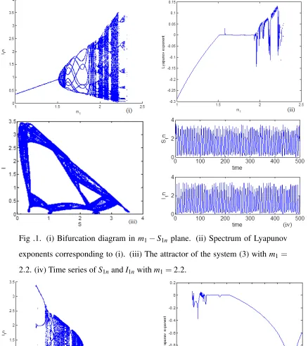
system (3) inm₁−S_1nspace is given in Fig. 1(i) to show the dynamical changes of susceptible and infective respectively as m1 varying. The spectrum of Lyapunov exponents of (3) with

respect to parameterm₁is given in Fig. 1(ii). Thus, we can see that the orbit with initial values approaches to the stable fixed pointP2form1<1.4 approximately, and Hopf bifurcation occurs

at m₁≈1.4. When increases to m₁≈2.3, (3) becomes stable. In Fig. 1(i), we observe the period-10, period-11 windows within the chaotic regions and boundary crisis atm₁≈2.3. For

m₁∈(1.9,2.3)the maximum Lyapunov exponents are mostly positive which corresponding to chaotic region. To well see the dynamics, the attractor in the system and time series of (3) with

m₁=2.2 and time series ofS_1n andI_1n are given in Fig. 1(iii) and (iv) respectively. For case (II), Fig. 2(i) is shows that there are period-6 windows, period-7 windows, period-8 windows

and invariant in the chaotic regions and boundary crisis at m₂ ≈0.92. Fig. 2(ii) shows that there is a part of Lyapunov exponents are positive which corresponding to chaotic region when

m2∈(0.65,0.75).

For case (III), Fig . 3(i) depicts that there are period-6, period-8 windows and invariant in the

chaotic regions, and two onsets of chaos atm₃≈0.32 andm₃≈0.68, , respectively. Fig 3(ii) shows a part of Lyapunov exponents are positive which corresponding to chaotic region when

m₃∈(0.1,0.2).

4.

CONCLUSION

In this paper, we investigate the behaviors of the SIS epidemic with logistic term as a

discrete-time dynamical system, and find many complex and new interesting dynamical phenomena.

Fig .1. (i) Bifurcation diagram in m₁−S_1n plane. (ii) Spectrum of Lyapunov exponents corresponding to (i). (iii) The attractor of the system (3) with m1=

2.2. (iv) Time series ofS_1nandI_1nwithm₁=2.2.

Fig. 3. (i) Bifurcation diagram inm₃−S_1nplane. (ii) The spectrum of Lyapunov exponents of (3) with respect to parameterm3.

analysis and numerical simulations have demonstrated that the model exhibits the variety of

dynamical behaviors, which include the discrete epidemic model undergoes transcritical

bifur-cation, flip bifurbifur-cation, Hopf bifurcation and chaos. The results show that there are different

dynamical behaviors between discrete system and its corresponding continuous system and the

results are different from [23]. Furthermore, chaos can cause the population to run a higher

risk of extinction due to the unpredictably [24-25]. Thus, how to control chaos in the epidemic

model is very important, which needs further consideration.

Acknowledgement

Project supported by the Youth Science Foundations of Education Department of Hebei Province

(No. QN2016265), Hebei Special Foundation ’333’ talent project (No. A20160 01123), and

Scientific Research Funds of Hebei Institute of Architecture and Civil Engineering

(Nos. 2016XJJQN03, 2016XJJYB05).

Conflict of Interests

The authors declare that there is no conflict of interests.

REFERENCES

[1] A. Gray, D. Greenhalgh, X. Mao, J. Pan, The SIS epidemic model with Markovian switching, J. Math. Anal.

Appl. 294 (2012), 496-516.

[2] X. Zhang, X. Liu, Backward bifurcation and global dynamics of an SIS epidemic model with general

[3] J. Linda, K. Nadarajah, M. Sherri, SIS epidemic models with multiple pathogen strains, J. Differ. Equ. Appl.

10 (2004), 53-75.

[4] J. Liu, T. Zhang, Bifurcation analysis of an SIS epidemic model with nonlinear birth rate, Chaos Soliton

Fract. 40 (2009), 1091-1099.

[5] D. Gao, S. Ruan, An SIS patch model with variable transmission coefficients, Math. Biosci. 232 (2011),

110-115.

[6] Y. Li, J. Cui, The effect of constant and pulse vaccination on SIS epidemic models incorporating media

coverage, Commun. Nonlinear Sci Numer. Simulat. 14 (2009), 2353-2365.

[7] Q. Wu, Y. Lou, Local immunization program for susceptible-infected-recovered network epidemic model,

Chaos 26 (2016), 023108.

[8] M. Frasca, K. Sharkey, Discrete-time moment closure models for epidemic spreading in populations of

inter-acting individuals, J. Theor. Biol. 399 (2016), 13-21.

[9] Q. Wu, X. Fu, Modelling of discrete-time SIS models with awareness interactions on degree-uncorrelated

networks, Physica A 390 (2011), 463-470.

[10] P. Salceanu, H. Smith, Persistence in a discrete-time stage-structured fungal disease model, J. Biol. Dynam.

3 (2009), 271-285.

[11] C. Wu, Existence of traveling waves with the critical speed for a discrete diffusive epidemic model, J. Differ.

Equations 262 (2016), 272-282.

[12] J. Li, Z. Ma, F. Brauer, Global analysis of discrete-time SI and SIS epidemic models, Math. Biosci. Eng. 4

(2007), 699-710.

[13] L. Allen, Y. Lou, A. Nevai. Spatial patterns in a discrete-time SIS patch model, J. Math. Biol. 18 (2009),

339-375.

[14] L. Li, G. Sun, Z. Jin, Bifurcation and chaos in an epidemic model with nonlinear incidence rates, Appl. Math.

Comput. 216 (2010), 1226-1234.

[15] Y. Xiao, L. Chen, A ratio-dependent predator-prey model with disease in the prey, Appl. Math. Comput. 131

(2002), 397-414.

[16] B. Liu, Y. Duan, S. Luan, Dynamics of an SI epidemic model with external effects in a polluted environment,

Nonlinear Anal-Real. 13 (2012), 27-38.

[17] N. Bairagi, S. Chaudhuri, J. Chattopadhyay, Harvesting as a disease control measure in an

eco-epidemiological system-A theoretical study, Math. Biosci.217 (2009), 134-144.

[18] G. Hu, X. Li, Stability and Hopf bifurcation for a delayed predator-prey model with disease in the prey,

Chaos, Soliton Fract. 45 (2012), 229-237.

[20] J. Guckenheimer, P. Holmes, Nonlinear oscillations, dynamical systems and bifurcations of vector fields, NY:

Spring Verlag; (1983).

[21] S. Wiggins, Introduction to applied nonlinear dynamical systems and chaos, Berlin: Springer-Verlag; (1990).

[22] P. Gaspard, M. Briggs, M. Francis, et al. Experimental evidence for microscopic chaos, Nature, 6696 (1998),

865-868.

[23] J. Li, J. Lou, M. Lou, Some discrete SI and SIS epidemic models, Appl. Math. Mech-Engl. 29 (2008),

113-119.

[24] A. Berryman, J. Millstein, Are ecological systems chaotic and if not, why not? Trends Ecol. Evol. 4 (1989),

26-28.

[25] M. Hassell, H. Comins, R. May, Spatial structure and chaos in insect population dynamics, Nature 353 (1991)