Oeschger Centre for Climate Change Research, University of Bern, Bern, Switzerland 3Department of Life Sciences, Imperial College London, Silwood Park, Ascot, SL5 7PY, UK Correspondence to: B. D. Stocker ([email protected])
Received: 3 July 2014 – Published in Geosci. Model Dev. Discuss.: 29 July 2014
Revised: 23 October 2014 – Accepted: 2 November 2014 – Published: 18 December 2014
Abstract. Simulating the spatio-temporal dynamics of inun-dation is key to understanding the role of wetlands under past and future climate change. Earlier modelling studies have mostly relied on fixed prescribed peatland maps and inunda-tion time series of limited temporal coverage. Here, we de-scribe and assess the the Dynamical Peatland Model Based on TOPMODEL (DYPTOP), which predicts the extent of in-undation based on a computationally efficient TOPMODEL implementation. This approach rests on an empirical, grid-cell-specific relationship between the mean soil water bal-ance and the flooded area. DYPTOP combines the simulated inundation extent and its temporal persistency with criteria for the ecosystem water balance and the modelled peatland-specific soil carbon balance to predict the global distribution of peatlands. We apply DYPTOP in combination with the LPX-Bern DGVM and benchmark the global-scale distribu-tion, extent, and seasonality of inundation against satellite data. DYPTOP successfully predicts the spatial distribution and extent of wetlands and major boreal and tropical peatland complexes and reveals the governing limitations to peatland occurrence across the globe. Peatlands covering large boreal lowlands are reproduced only when accounting for a posi-tive feedback induced by the enhanced mean soil water hold-ing capacity in peatland-dominated regions. DYPTOP is de-signed to minimize input data requirements, optimizes com-putational efficiency and allows for a modular adoption in Earth system models.
1 Introduction
Changes in the extent of wetlands affect the climate sys-tem biogeophysically and biogeochemically. The surface-to-atmosphere exchange of energy and water is fundamentally altered over flooded areas (Gedney and Cox, 2003; Krin-ner, 2003; Moffett et al., 2010) and wetland ecosystems play a disproportionately important role for the atmospheric methane (CH4) and carbon (C) budgets (Tarnocai et al., 2009; Yu et al., 2010). Today, 175–217 Tg CH4, or 20–40 % of total annual emissions originates from wetlands (Kirschke et al., 2013) and the spatio-temporal variability of wetland extent exerts direct control on the seasonal and interannual changes in CH4 emissions and its atmospheric growth rate (Bloom et al., 2010; Bousquet et al., 2006). Changes in the distribution and productivity of wetlands were most likely a major driver for CH4variations during glacial–interglacial cycles and millennial scale climate variability during the last glacial period (Spahni et al., 2005; Schilt et al., 2010).
Peat-lands not only contribute about 40–50 Tg CH4-C to an-nual CH4 emissions (Spahni et al., 2011), but also store 500±100 Gt carbon (Gt C) (Yu et al., 2010), which corre-sponds to about a fifth of the total global terrestrial C storage (Ciais et al., 2013). In contrast to mineral soils, peatlands continue to accumulate C on millennial timescales owing to the extremely slow decomposition rates and the associated long-lasting legacy effects of climatic shifts that occurred even millennia before today (e.g. the disappearance of the Laurentide ice sheet in the course of the last deglaciation).
Accounting for the pivotal role of wetlands for global greenhouse-gas (GHG) budgets, representations of wetland biogeochemical processes are implemented in land models to hindcast observed past variations and predict future tra-jectories in atmospheric CH4 and the terrestrial C balance (Singarayer et al., 2011; Spahni et al., 2011; Kleinen et al., 2012; Melton et al., 2013; Zürcher et al., 2013). Dynamic global vegetation models (DGVMs) and terrestrial biosphere models (TBMs), often applied as modules to represent land processes in earth system models, resolve relevant processes to simulate terrestrial GHG emissions and uptake in re-sponse to variations in climate and CO2 (McGuire et al., 2001), while land surface models (LSMs) are applied to sim-ulate biogeophysical processes associated with the interac-tion between the land surface and the atmosphere. DGVMs, TBMs, and LSMs, hereafter referred to as land models, of-ten rely on a fixed prescribed exof-tent of wetlands and peat-lands. However, predictive model capabilities with respect to the spatial distribution of wetlands and peatlands are crucial when applying models to boundary conditions beyond the present-day state, i.e. when their spatial distribution is sub-stantially different from present-day observational data. Also on shorter timescales, the seasonal and inter-annual variabil-ity of wetland extent appears key to explaining the observed variations in CH4growth rates (Bloom et al., 2010; Bousquet et al., 2006; Kirschke et al., 2013). In other words, predic-tions of wetland GHG emissions rely not only on the evolu-tion in the flux rates per unit area, but importantly also on changes in the areal extent of wetlands.
The challenge for global model applications with rela-tively coarse model grid cells is that even the large-scale hy-drological characteristics are determined by the unresolved sub-grid scale topography. Diverse wetland extents simulated by current state-of-the-art land models, applied for bottom-up CH4 emissions estimates, underline this standing issue (Melton et al., 2013; Wania et al., 2013). Different recent ef-forts to include dynamical wetland schemes into land models (Gedney and Cox, 2003; Ringeval et al., 2012) are founded on the concepts of TOPMODEL (Beven and Kirkby, 1979). This approach was initially developed to dynamically sim-ulate contributing areas for runoff generation in hydrologi-cal catchments. It relies on a topographic index represent-ing the “floodability” of an areal unit within a given river catchment. Using this sub-grid scale topography informa-tion, TOPMODEL accounts implicitly for the redistribution
of soil water along topographical gradients within a river catchment and predicts the area at maximum soil water con-tent. Neglecting the temporal dynamics of water mass redis-tribution effects through a channel network topology (river routing), the area at maximum soil water content is used as a surrogate for the inundated area fraction, thereafter referred to asf. TOPMODEL-based implementations have proved successful at capturing the broad geographic distribution of wetlands and their seasonal variability (Gedney and Cox, 2003; Ringeval et al., 2012).
Recently, Kleinen et al. (2012) combined TOPMODEL with a model for peatland C dynamics to predict the boreal peatland distribution and simulate their C accumulation over the past 8000 yr (8 kyr). The rationale for their modelling approach is that conditions for peatland establishment and growth are limited to areas where water-logged soil condi-tions are sufficiently frequent. Peatland distribution is thus co-limited byf, which is simulated by TOPMODEL.
Here, we present the Dynamical Peatland Model Based on TOPMODEL (DYPTOP). It makes use of the TOPMODEL approach to establish a relationship between the water table depth and the flooded grid-cell area fraction. Once estab-lished, this grid-cell-specific relationship is represented by a single analytical function and a set of four grid-cell-specific parameters (provided in the Supplement). This function is used to dynamically predict the inundated area fractionf in combination with the water table depth as simulated by a land model. This simplification reduces required input data, en-hances numerical efficiency, and facilitates the adoption of dynamical inundation prediction schemes into land models.
DYPTOP combines this inundation model with a model determining suitability for peatland growth conditions to simulate their spatial distribution and temporal change. This is founded on the approach of Kleinen et al. (2012) but in-cludes a set of modifications to resolve the challenge of predicting the observed spatial heterogeneity of the global peatland distribution across the boreal region. In particular, peatland distribution is considered to be limited by the per-sistency of inundation, rather than its mean. Furthermore, DYPTOP accounts for the feedback between inundation dy-namics, peatland establishment, and the modification of the regional hydrology by the distinct hydraulic properties of organic peatland soils. The present model is designed to account for the temporal inertia of lateral peatland expan-sion, enabling future investigations of the dynamics of peat-land shifts over palaeo-timescales and under future climate change scenarios. In addition, the present study extends the scope of Kleinen et al. (2012) to the global scale, attempts to predict the occurrence of peatland soils also in tropical and sub-tropical ecosystems, and relies on plant physiology pa-rameterizations of peatland-specific plants.
DYP-and water cycles through photosynthesis DYP-and evapotranspi-ration. Plant functional types (PFTs) are the basic biological unit and represent different life forms (grasses, trees, mosses) and combination of plant traits (needle-leaved, broad-leaved, etc.). The distribution of PFTs is simulated based on a set of bioclimatic limits and by plant-specific parameters that gov-ern the competition for resources. Here, we apply the LPX-Bern version 1.2, a further development of the LPJ-DGVM (Sitch et al., 2003). It accounts for the coupled cycling of C and nitrogen (N), whereby net primary productivity (NPP) is limited by the availability of explicitly simulated inorganic N species following Xu-Ri and Prentice (2008).
Each grid cell in LPX-Bern is separated into fractions rep-resenting different land classes (tiles) where C, N, and water pools are treated separately. Upon any change in the tiles’ fractional area, water, C, and N are reallocated, conserv-ing the respective total mass (see Strassmann et al., 2008; Stocker et al., 2014). Here, we explicitly distinguish between natural land with mineral soils (fmineral), peatlands (fpeat), and former peatlands, now treated as mineral soils (foldpeat). We describe how the simulated soil water balance and a di-agnosed inundation area (see Sect. 3) can be used to predict changes in the fractional areasfmineral,fpeat, andfoldpeat in response to changes in climate and CO2 (see Sect. 4). De-pending on the model application, LPX-Bern land classes may additionally distinguish between land with primary vs. secondary vegetation, croplands, pastures, and built-up areas (see Stocker et al., 2014). These model features are not acti-vated in this study.
Ringeval et al. (2014) applied an alternative version of LPX-Bern (version 1.1) to simulate separate C dynamics on floodplains which are represented by a separate land class (tile). This feature is not used for the present study as the focus here is on the spatial dynamics of peatlands and any additional grid-cell tile comes at a substantial computational cost.
Biogeochemical processes and the water balance are sim-ulated using distinct parameterizations on the different grid-cell tilesfmineralandfpeat. All parameterizations and param-eters are identical forfmineralandfoldpeat. Onfpeat, we apply
et al., 2014). Additionally, we removed the upper tempera-ture limitation of the other peatland-specific PFTs, already used in previous studies (Graminoids, Sphagnum) to permit their growth outside the boreal region. Representations for the interaction of the C and N cycles are implemented in the peatland-specific model part as described in Spahni et al. (2013). However, we updated the prescribed soil C : N ratio for the peatland PFTs (C : N ratios for sedges=35.87, sphag-num moss=82.35, other woody PFTs=50.98) according to Loisel et al. (2014).
Parameterizations and parameter values applied for C and N cycling on natural land on mineral soils (fmineral and
foldpeat) are largely identical to previous applications of LPX-Bern version 1.0 (Stocker et al., 2013; Spahni et al., 2013). Changes since version 1.0 include the application of an improved litter decomposition parameterization following Brovkin et al. (2012). Additionally, the temperature govern-ing soil organic matter decomposition in LPX-Bern version 1.2 is computed based on the simulated temperature profile (instead of a single value representing 25 cm depth, Sitch et al., 2003), weighted by a logarithmic soil C profile, fit-ted to decreasing C density with depth as measured by Wang et al. (2010) on forest, grass, shrub, and desert ecosystems.
3 A TOPMODEL implementation to model the distribution of wetlands
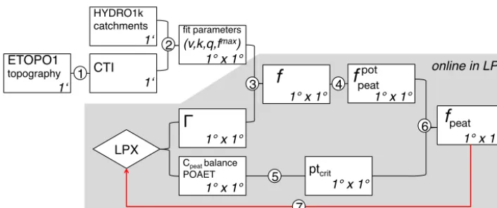
Figure 1 illustrates the information flow in DYPTOP. Steps 1–3 determine the inundated area fractionf and are described in Sect. 3. Steps 4–6 determine the peatland area fractionfpeatand are described in Sect. 4.
3.1 Topography and inundated area fraction
ETOPO1!
topography!
1‘!
!
Γ
!
1° x 1°!
!
CTI! 1‘!
HYDRO1k!
catchments! 1‘!
!
fit parameters!
(v,k,q,fmax) !
1° x 1°!
!
LPX! !
Cpeat balance!
POAET!
1° x 1°!
!
! !
!
1° x 1°!
!
!
!
!
1° x 1°!
!
1
2
3
!
!
1° x 1°!
!
6
!
ptcrit! 1° x 1°!
!
f
peatpot€
f
peat 45
online in LPX!
7
f
Figure 1. Overview of information flow of DYPTOP. Boxes represent spatial fields of the respective variables, given at the spatial resolution
as indicated in the lower right edge of each box. (1) Compound topographic index (CTI) values are derived from the ETOPO1 (2013) high resolution topography data set using the R library “topmodel” (Buytaert, 2011). (2) Fit parameters(v, k, q)are derived by applying the least-squares fitting algorithm “nls” in R (R Core Team, 2012) to best reproduce the “empirical” relationship between the water table position (0) and the flooded area fraction (f) as derived from the ETOPO1 data and Eqs. (2) and (3).fmaxis the maximum area fraction that is allowed to be flooded within a grid cell and is computed by using a globally uniform threshold value for CTI (CTImin) below which flooding is prohibited (Eq. 4). (3)(v, k, q, fmax)are prescribed to LPX-Bern to predictf as a function of0, which is interactively simulated in LPX-Bern. (4) The potential, hydrologically viable, peatland extentfpeatpot is set to the minimum of theN months with highest inundation over the preceding 31 years (see Eq. 13). (5) Peatland C balance criteria and the ratio of precipitation over actual evapotranspiration (POAET) are used to determine whether a peatland can establish in the respective grid cell. (6) If criteria are satisfied, the actual peatland areafpeat fraction converges over time tofpeatpot. (7) The presence of peatlands affects the local soil water storage and retention capacity and thus exerts a feedback via the mean grid-cell water table position0andf.
relationship is provided by the sub-grid scale distribution of the CTI. In the following, we refer to “pixels” (indexi, here ∼1 km) as the grid cells within each model grid cell (index
x, here 1◦×1◦). The CTI determines how likely a pixel is to get flooded (“floodability”). The higher the value, the higher its floodability. It is defined as
CTIi=ln(ai/tanβi) , (1)
whereairepresents the catchment area per pixeli, i.e. the
to-tal area that drains into/through the respective pixel.βirefers
to the slope of the pixel. Here, CTI values are derived from the ETOPO1 high resolution (1 arc min) topography data set (ETOPO1, 2013) and are calculated using the R library “top-model” (Buytaert, 2011) (Step 1 in Fig. 1). Deriving CTI fields from a topography data set instead of relying on avail-able CTI products allows us to extend CTI fields to areas below the present-day sea level for applications on palaeo-timescales.
Following the TOPMODEL approach, we calculate the threshold CTI∗xin each grid cellx, as a function of the grid-cell-mean water table position 0x. Here, 0x is in units of
mm above the surface. All pixelsiwith CTIi >CTI∗xare at
maximum soil water content. Here, this is interpreted as the respective pixel being flooded. CTI∗xis defined by
CTI∗x=CTIb−M·0x, (2)
where CTIbis the arithmetic mean CTI value, averaged over
the entire primary catchment areab in which the respective
pixel is located. This is a simplification in case two pix-elsi and j exist where CTIi >CTIj, and i lies upstream
fromj. In this case, the relative floodability of CTIi is
af-fected by the fact that CTIj has a low floodability (low CTI
value), when in effect there is hardly any influence as CTIj
lies downstream from CTIi. However, CTI values
gener-ally increase downstream (drainage areaa increases), hence CTIi>CTI∗>CTIj is not frequent. Note that the
catch-ment area may extend beyond the model grid cell in which the pixel is located. The catchment area data set is from HYDRO1K (2013). Thus, whether a pixel is flooded, hence CTIi>CTI∗x, depends on the floodability of other pixels in
the same catchment area.M is handled here as a free (and tunable, see Table 1 and Sect. 7.1.1) parameter. More strictly,
Mdescribes the exponential decrease in soil water transmis-sivity with depth (see Beven and Kirkby, 1979).
Accounting for the full topographical information con-tained in the CTI values within a grid cellx, the flooded area fractionfˆx within the respective grid cell is determined by
the total area of all pixels within grid cellxwith CTIi being
Figure 2. “Empirical” (black) and fitted (red) curves relating the grid cell mean water table position (0) to the flooded fraction of this grid cell. A mountainous grid cell (left, centred at 101.25◦W, 22.5◦N) and a flatland grid cell (right, centred at 93.75◦W, 20◦N) are shown as examples. Vertical blue lines illustrate0for each month as simulated by LPX for the period 1901–2012 (see Sect. 5.2).
Table 1. DYPTOP model parameters.
Parameter Value Description/Reference
M 8 TOPMODEL parameter, Eq. (2)
CTImin 12 Minimum CTI for floodability, Eq. (3)
λ 2 Exponential correction factor for effective soil depth, Eq. (11)
N 18 Minimum number of months with inundation, Eq. (13)
r 0.01 yr−1 Maximum relative peat expansion/contraction rate, Eq. (14) POAET∗ 1.0 Minimum precipitation-over-actual-evapotranspiration, Fig. 3 Cpeat∗ 50 kg C m−2 Minimum peat amount, Fig. 3
dCpeat∗
dt 10 g C m
−2yr−1 Minimum annual peat accumulation, Fig. 3
position. Thus we get ˆ
fx=
1
Ax X
i A∗i,
withA∗i =
(
Ai if CTIi≥max(CTI∗x,CTImin) 0 if CTIi<max(CTI∗x,CTImin),
(3)
and hence for the maximum inundated area fraction in grid cellx:
fxmax= 1
Ax X
i A∗i,
withA∗i =
(
Ai if CTIi≥CTImin 0 if CTIi<CTImin.
(4)
Ax is the total surface area of grid cellx, andiruns over
all pixels located within the respective grid cell. The choice of CTIminaffects the maximum possible extent of inundated land within a grid cell and is further discussed in Sect. 7.1.1. The distribution of CTI values within a given grid cell and the catchment mean CTI determines the inundated area
frac-POAET > 1
dCpeat dt >10 gCm
−2yr−1 C
peat>50 kgCm
−2
Y
ptcrit = FALSE
ptcrit = FALSE
N
N N
ptcrit = TRUE
Y
ptcrit = TRUE
Y
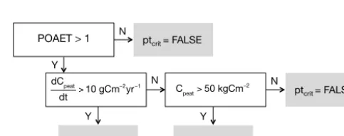
Figure 3. Illustration of decisions determining the criterion for
peat-land expansion ptcrit. The decision tree is evaluated starting in the upper-left box and variables are computed using the peatland bio-geochemistry model of LPX-Bern (Spahni et al., 2013) based on LPJ-WHyMe (Wania et al., 2009a, b).
tionfˆxof this grid cell for each0x(see Eq. 2). This
relation-ship is distinct for each grid cell and is illustrated in Fig. 2 for two example grid cells. Having to rely on the full information CTIi is computationally costly due to the (necessarily) high
Instead of fitting a gamma function to the distribution of CTIi, as has been done earlier (Sivapalan et al., 1987), we
directly define a function 9 fitted to the “empirical” rela-tionship9ˆ betweenfˆand0.9ˆ is established by evaluating
ˆ
f using Eqs. (2) and (3) for a sequence of0spanning a plau-sible range of values (here from−2000 mm to 1000 mm) and for each grid cellx individually.9ˆ generally has a shape as displayed for an example grid cell in Fig. 2 (black curve) and can be approximated by an asymmetric sigmoid func-tion 9 (red curve) with three parameters(v, k, q)x and for
CTImin=0. Here, we apply monthly mean values of 0as computed by LPX for each monthmand grid cellx:
9x(0x,m)=
1+vx·e−kx(0x,m−qx) −1/vx
. (5)
We determine parameters (v, k, q)x using the non-linear
least-squares fitting algorithm “nls” in R (R Core Team, 2012) (Step 2 in Fig. 1). Note that9xis distinct for each grid
cellx, as reflected by the values of parameters(v, k, q)x.
Ad-ditional information is contained in the cut-off value CTImin that determines the maximum flooded area fraction fxmax
(see Eq. 4). It follows (Step 3 in Fig. 1) that:
fx,m=min(9x(0x,m), fxmax). (6)
The two-dimensional (longitude×latitude) fields
(v, k, q, fmax)x carry the full information, here on
a 1◦×1◦ resolution, and can be used as input for any global model to predict the (monthly) value of the area fraction that is flooded (fx,m) from the (monthly) water
table position0x,m in grid cell x. These data are provided
in the Supplement and may be applied in combination with an implementation of Eqs. (6) and (5). An example code programmed as a subroutine in FORTRAN is also provided in the Supplement.
In conclusion, the concept presented here can be de-scribed by the re-mapping of9 to9ˆ, where the information
(CTI, M,CTImin)is reduced to(v, k, q, fxmax)x:
(CTI, M,CTImin)7−→(v, k, q, fxmax)x. (7)
The choice of CTIminandMdetermines the parameter set
(v, k, q, fxmax)x. The large array CTI is reduced to optimize
computational costs. In Sect. 7.1.1, we describe howMand CTIminare constrained using observation-based data.
The water table position (0) is the ultimate predictor vari-able forf and is calculated online by LPX-Bern. How0is defined exactly may depend on the nature of the soil water model implemented in the respective DGVM, and results for
f thus depend on the DGVM-specific predictions of0. The following subsection describes the definition of0 in LPX-Bern. All results shown in Sect. 6 are to be interpreted with respect to this DGVM-specific definition of0.
3.2 Definition of the water table position
The grid-cell-mean water table position0 is calculated as a grid-cell fraction-weighted mean,
0=fpeat·0peat+fmineral·0mineral+foldpeat·0oldpeat, (8) wherefmineral,fpeat, andfoldpeat are the grid-cell area frac-tions as described in Sect. 2.
The simulated inundated area fractionf is governed by model predictions of the water table position0. In the model for peatland-specific biogeochemistry,0peatis the key vari-able determining soil oxygen status and organic matter de-composition. It is explicitly simulated as described in Wa-nia et al. (2009b) (their Eq. 22). The definition of 0peat accounts for the particular hydraulic properties of peatland soils. This tends to constrain seasonal0peatvariations to gen-erally higher values than0mineralthrough mechanisms of en-hanced soil water storage and retention and reduced runoff.
On non-peatland soils (fmineral and foldpeat), no explicit variable representing the water table position 0mineral and
0oldpeat is available in LPX-Bern. In the following, we de-fine0mineraland0oldpeat as an index that is suitable for the present application.
On non-peatland soils, the water balance, surface and drainage runoff are modelled by a relatively simple “two-bucket” approach based on the original LPJ (Sitch et al., 2003). The change in water content of the upper layer is given by the balance between precipitation, snow melt, runoff, per-colation to the lower layer, evaporation, and the fraction of plant transpiration extracted from this layer. The change in the lower layer results from percolation from the upper layer, losses to ground water, and transpiration.
The soil water model version used here has been extended to account for heat diffusion, melting and thawing across eight soil layers, while the soil water content in the two buck-ets is uniformly distributed within the upper and lower four layers, respectively. Soil moisture – the governing variable for plant water status – is simulated as a scalar index for each bucket (see Eq. 9) as described in Sitch et al. (2003). This “mixed” approach allows for simulating the restric-tion of percolarestric-tion when frozen soil layers are present while still maintaining computational efficiency (as compared to a model where the full water budget and its vertical diffu-sion/percolation are resolved for each soil layer).
The soil moisture scalarθi in bucketivaries between 0 at
permanent wilting pointWPWP and 1 at field capacityWFC and is defined as
θi=
Wi−WPWP
WFC−WPWP
. (9)
Figure 4. Ranked monthly flooded area fraction f for a 31 years period (1982–2012) and for two regions comprising the Hudson Bay Lowlands (70–110◦W/48–58◦N, top) and the West Siberian Lowlands (50–180◦E/60–65◦N, bottom). Each line represents one grid cell. The monthly flooded area fractions are compared to observation-based data of peatland area fraction (Tarnocai et al., 2009) by colouring the line for each grid cell accordingly (see colour key).f is calculated as a function of the water table position computed by LPX for mineral soils only (left) and for the grid-cell area fraction-weighted mean0(right, see Eq. 8), i.e. before and after peatland establishment. The vertical blue line is drawn at ranked months=18, representing the model parameterN in Eq. (13). The intersect of a given line with the blue line definesfpeatpot in the respective grid cell.
below a certain level0∗=WFC/φ1z, determined by the soil depth1z, the porosityφ, andWFC. This may hinder an ap-plication of such models in combination with TOPMODEL, as argued in Ringeval et al. (2012).
Here, the monthly updated “water table position” in min-eral soils, 0mineral,m, is defined as an index consisting of
the combination of monthly mean water-filled pore space
(Wl·1zl/φ), the monthly total runoff, and the soil depth,
modified by the presence of frozen soil layers:
0mineral,m=
1
Nm
Nm
X
d=1
−zl0,d+
l0
X
l=1
Wl,d· 1zl
φ !
+runoffm
φ . (10)
Subscriptsm,d, andlrepresent months, days, and soil lay-ers,Nmis the number of days for monthm,l0is the number of the layer just above the first frozen soil layer counted from the top (surface,l=1),Wl,d is the daily updated soil liquid
water plus ice fraction in layer l,zl is the soil layer
thick-ness, φis the porosity (uniform over depth), and runoffmis
the sum of monthly total surface and drainage runoff.zl0,d is
the soil depth, reduced to the depth at the upper boundary of the uppermost frozen soil layer, if any is present. Otherwise, it is set to the nominal soil column depthzmax= −2000 mm. This mimics the amplified susceptibility to flooding on (par-tially) frozen soils.
However, Eq. (10) may overestimate flooding when the liquid soil water above the uppermost frozen soil layerl0is low. Therefore, we applied an effective soil depthzl∗
0,dinstead ofzl0,d in Eq. (10), defined as
z∗l
0,d=zl0,d−(zl0,d−zmax) e
−λ θd . (11)
θd is the daily updated soil moisture index (Eq. 9), averaged
over all soil layers abovel0, andλ is a parameter, here set to 2 (see Sect. 7.1.1). Equation (11) guarantees that at high soil moisture, the effective soil depthz∗l
0,dis equal tozl0,d. At low soil moisture,z∗l
4 Representing peatland distribution
Lateral expansion and contraction of peatland areas are sim-ulated dynamically as a convolution of (i) peatland carbon (C) balance conditions as simulated by LPX and (ii) flood-ing persistency as simulated by the TOPMODEL imple-mentation. Peatland C balance conditions are simulated for an area fraction fpeatmin=0.001 % in each grid cell globally. This value is small enough not to significantly affect the global C balance (0.0005 % of global peat C according to results presented in Sect. 6), but large enough to provide an effective “seed” for peatland establishment and expan-sion once conditions for peatland establishment are met (It takes 1158 years fromfpeatmin=0.001 to 1 at 1 % yr−1 expan-sion rate, see Sect. 4.3). On this minimum area, we apply the peatland-specific model for C dynamics and the water bal-ance as mentioned in Sect. 2.
4.1 Peatland establishment criteria
In each simulation year, a hierarchical series of conditions for peatland expansion or shrinking are evaluated for each grid cell, and the boolean variable ptcritis set (ptcrit=“true” if the conditions are met and “false” if they are not; see Fig. 3, and Step 4 in Fig. 1). The primary condition is re-lated to the ecosystem water balance, represented by annual total precipitation divided by (over) annual total actual evap-otranspiration (POAET). Global peatland occurrence analy-ses (Gallego-Sala and Prentice, 2013; Charman et al., 2013) have revealed the limiting role of precipitation over
equi-librium evapotranspiration. Here, we apply a threshold of
POAET∗=1 to limit peatlands to regions with a positive water balance. Simulated actual evapotranspiration is gov-erned by the water table position and varies between 79.5 and 109.5 % of equilibrium evapotranspiration (EET). This fol-lows from the definition given in Wania et al. (2009a) (their Eq. 23). EET is defined after Prentice et al. (1993) (their Eq. 5).
If this first condition is met, C balance criteria suitable for peatland expansion are satisfied either when peatland soil C accumulates with a multi-decadal average rate of more than 10 g Cm−2yr−1, or as long as total soil C exceeds the thresh-old of 50 kg m−2. All criteria are computed for each grid cell (note thatfpeat≥fpeatminfor all grid cells) for the current year by averaging the simulated C balance variables and POAET over the preceding 31 years. This is to reduce interannual variability in ptcrit, which is driven by interannual variabil-ity in climate (a 31 years time series is repeatedly prescribed during the spin-up; see Sect. 5.2).
4.2 Potential peatland area fraction
The potential peatland area fraction fpeatpot defines the max-imum possible peatland extent within each grid cell. fpeatpot
is approached during peatland expansion in the case ptcrit
is “true”, taking account of temporal inertia (see Eq. 14). It is determined independently from ptcritand captures both the flooding persistency and the seasonal maximum extent of flooding within the respective grid cell (see Step 5 in Fig. 1). The algorithm applied to determinefpeatpot can be described as follows. For each grid cell, all monthly values of the inun-dated area fractionfmof the preceding 31 years are sorted in
descending order. The sorting transforms the vectorftof∗.
f=(f1, . . .f372)→f∗= f1∗, . . .f
∗
372.
(12) The potential peatland area fractionfpeatpot is then defined as
fpeatpot =fN∗, (13)
whereN is a constrainable parameter. This procedure ac-counts for inundation persistency as a determining factor for peatland extent, i.e. fN∗ defines the area fraction that is inundated at leastN months during 31 years. We inves-tigated fpeatpot, applying values N=(10,15,18,20,25) (see Sect. 7.2.2). Figure 4 illustrates the sorted vectorsf∗, for two regions.
4.3 Lateral expansion and contraction
Finally, the actual peatland area fractionfpeat is simulated as a convolution of ptcritandfpeatpot. During the transient sim-ulation (after model spin-up), the annually updatedfpeat(t ) gradually expands towardsfpeatpot as long as ptcritis “true”, and contracts tofpeatmin, when ptcritis “false”. To account for iner-tia in lateral peatland expansion and contraction, the relative areal change rate is limited to 1 % yr−1(r=0.01 yr−1).
fpeat(t )=
min
(1+r)·fpeat(t−1), fpeatpot
, ptcrit=true
max
(1−r)·fpeat(t−1), fpeatmin
, ptcrit=false.
(14) Upon peatland contraction, the areafpeat(t−1)−fpeat(t ) is allocated tofoldpeat, and expanding peatlands first expand intofoldpeat. This guarantees that C and N mass on grid-cell area fractions that have never (in the course of the simulation) been covered by peatlands are kept track of separately, and prevents C, N, and soil water from being redistributed across the entire grid cell. At any given timetduring the simulation,
foldpeat(t )is thus determined by the maximum peatland area fraction in all preceding years in each grid cellxindividually:
foldpeat,x(t )=max(fpeat,x(t=0, . . . t ))−fpeat,x(t ). (15)
In LPX-Bern, the monthly varying inundated area fraction is used not only to derive annually varying fpeat, but also to simulate monthly varying contributing areas for methane emissions from inundated mineral soils (finund). No results for simulated methane emissions are presented in this paper. While contributing areas for methane emissions from peat-lands are constant within one year and equal tofpeat,finund is defined by
also illustrated byfpeat,0vs.fpeatin Figs. 8 and 9.fpeatthus imparts a positive feedback via0and the flooded area frac-tion f through mechanisms of enhanced soil water storage and retention and reduced runoff. Under transiently chang-ing climatic conditions, this leads to a hysteresis behaviour: once peatlands are established, they can persist even under conditions where no new peatlands would form.
5 Experimental setup and benchmark data
5.1 Model spin-up procedure for peatland area fraction Due to the slow turnover times of soil organic matter, pool size equilibration under given environmental conditions is at-tained only on timescales of 103years for mineral soils and around 104 years for peatland soils. Instead of running the model forward over several millennia, we apply an analyti-cal solution to shorten the model spin-up. Equilibrium soil C and N pool sizes (C∗) in models with first-order decay ki-netics are defined by their inputs by litter fall (I), and their turnover timesτ:
C∗=I · τ. (17)
This pool equilibration is applied in spin-up year 1000 for mineral soil pools by averagingI andτ over the preceding 31 years.
Complete equilibration of pools cannot be applied for peatlands due to their turnover times being on the same time scale as their age since initiation. The peatland-specific model spin-up is divided into three phases. Pool sizes are initialized to be empty. In the first phase (here, spin-up years 1–999), the soil and litter C and N pools gradually but slowly increase in response to litter inputs. At the end of phase one, the soil pools are scaled up to near-equilibrium. We assume that present-day litter inputs have been sustained for the pre-ceding t∗=12 000 yr and analytically calculate the respec-tive peatland soil pool sizes as
C∗=(1−e−t∗/τ)·I · τ. (18)
This spin-up procedure ensures that mineral soils are fully equilibrated, while peatland soils with long turnover times continue to slowly increase in size by the end of the spin-up. 5.2 Simulation protocol
Coupled C and N dynamics and the soil heat diffusion and water balance in terrestrial ecosystems are simulated by LPX-Bern, Version 1.2 (Stocker et al., 2013). This model version is extended to include the DYPTOP model as de-scribed in Sects. 3 and 4. Standard parameters are chosen as discussed further in Sects. 7.1.1 and 7.2.2:M=8 in Eq. (2), CTImin=12 in Eq. (4), N=18 in Eq. (13), and λ=2 in Eq. (11).
Two model simulations were carried out. In the first (S0), peatlands are not accounted for (peatland area fraction is zero everywhere and at all times). In this simulation, the inunda-tion fracinunda-tionf does not affect the carbon dynamics, nor any other model state variable. In this simulation, 0=0mineral and the potential peatland area fraction before peatland es-tablishmentfpeatpot can be quantified.
In the second simulation (S1), peatlands are accounted for andf is used to determine the peatland area fraction follow-ing the method outlined in Sect. 4. In this simulation,0is calculated as the grid-cell area fraction-weighted average0
in mineral and peatland soils (see Eq. 8), and the potential peatland area fraction after peatland establishmentfpeatpot can be quantified.
Figure 5. Top row: estimated (left, Prigent et al., 2007) and simulated (right) annual maximum inundated area fraction, averaged over 1993
to 2004. The fraction of simulated established peatlands (see Fig. 7) is subtracted from the simulated inundation area fraction for a better comparison with GIEMS. The data shown here thus correspond tofinund(Eq. 16). Note the non-linear scale. Bottom row: estimated (left) and simulated (right) month with maximum inundation extent. Months are numbered from 1 (January) to 12 (December). Boxes define regions for which mean seasonality is analysed in Fig. 6. Blank land grid cells in the map at the bottom-left represent locations where the inundation area is zero throughout the year.
a spin-up under present-day conditions appears less appro-priate.
5.3 Benchmark data 5.3.1 Inundation area
Prigent et al. (2007) combined satellite data from passive microwave, active microwave (scatterometer), altimetry, and Advanced Very High Resolution Radiometry (AVHRR) into a “multisatellite” method to estimate monthly inundated ar-eas over multiple years and covering the entire globe. The up-dated data set by Papa et al. (2010) is applied here and covers years 1993–2004. This is the first and – to date – only data set that represents the seasonal and inter-annual dynamics of in-undation areas. The original data are on a 0.25◦×0.25◦ spa-tial resolution (at the Equator) and have been regridded for the present application using area-weighted averages (see Fig. 5). Hereafter, “GIEMS” refers to the data set by Papa et al. (2010), which is based on Prigent et al. (2007).
This data set provides information on the temporal vari-ability of inundation that compares well with related hy-drological variables (Prigent et al., 2007). However, com-pared with static wetland maps, the satellite-derived data set of GIEMS notoriously underestimates the inundated area fraction in regions with small and dispersed flooding that amounts to less than about 10 % of the grid-cell area (Prigent et al., 2007). A comparison of GIEMS inundation areas with the Global Lakes and Wetlands Database (GLWD, Lehner
and Döll, 2004) suggests that areas classified in GLWD as peatlands (“Bog, Fen, Mire”), “wetlands”, and “Swamp Forest, Flooded Forest” are generally under-represented in GIEMS. This mostly affects regions in boreal Canada, East-ern Siberia, WestEast-ern Amazonia, Congo, and the Tibetan Plateau. This is confirmed by a study focusing on the Ama-zon catchment and relying on synthetic aperture radar in combination with airborne videography (Melack and Hess, 2010). This regional data product suggests higher inundation area fractions than other remotely sensed data (∼15 % aver-aged over the Amazon catchment). Detecting surface water under dense vegetation generally appears to be challenging due to microwave signal attenuation.
5.3.2 Peatland distribution
Tarnocai et al. (2009) mapped soils in permafrost regions across the northern circumpolar region. For the present study, we converted this data set to a gridded field so that the frac-tion within each 1◦×1◦ grid cell covered by either histels
pat-total in
undated area (1000 km
JAN MAR MAY JUL SEP NOV 0
200 400
total in
undated area (1000 km
JAN MAR MAY JUL SEP NOV 0
20 40
total in
undated area (1000 km
JAN MAR MAY JUL SEP NOV 0
100
Figure 6. Observed and simulated mean seasonality (mean over 1993–2004, based on simulation S1) of total inundated area by region (AF –
Africa, NA – North America, SI – Siberia, IC – India/China and others, SEA – South East Asian Islands, SA – South America). Outlines of these regions are given by the boxes in Fig. 5, bottom. Blue bars in plots for NA and SI represent simulated snow cover as a fraction of annual maximum (blue=1, white=0). The fraction of simulated established peatlands (see Fig. 7) is subtracted from the simulated inundation area fraction for a better comparison with GIEMS. Dashed red lines represent simulated inundation additionally corrected for snow cover (areas with with snow cover depth>30 mm snow water equivalents are masked out) and rice cultivation areas (using the maximum of simulation inundation and wet rice cultivation area after Leff et al. (2004) withf=max(frice, f )).
terns at a high resolution (relying on maps of 1:250 000 to 1:3 000 000 scale), this transformation appears pragmatic.
The same issue applies to the alternative peatland distribu-tion benchmark data set by Yu et al. (2010). These authors provide a map that delineates “peatland-abundant” regions, i.e. where peatlands cover at least 5 % of the landmass. Orig-inal binary data on 0.05◦×0.05◦are regridded here to repre-sent the fractional area with significant peatland cover frac-tion on the 1◦×1◦grid applied for the present simulations. This information is not directly comparable to the fractional peatland area but should help here to visualize the global dis-tribution of peatland-dominated regions also in areas outside regions affected by permafrost. The peatland area fraction benchmark data sets are illustrated in Figs. 7, 8, and 9.
6 Results
6.1 Inundation areas
Simulation results suggest that major seasonally inundated areas can be found at high northern latitudes in the Cana-dian and Siberian tundra with values off around 25 % and along major rivers in tropical and sub-tropical regions (west-ern Amazon, Ganges/Brahmaputra, Fig. 5). The location and extent of these major simulated inundated areas agree well with observational data (GIEMS), but are underestimated in regions where wet rice cultivation is abundant as rice
culti-vation is not accounted for in the present simulations (south and east Asia).
On peatlands, the water table is generally below the sur-face, which implies that remotely sensed data do not detect or underestimate inundation areas in regions dominated by peatlands. Indeed, the GIEMS data set suggests no signifi-cant inundation in regions dominated by peatlands.
Wetland fractionsf of around 10 % are simulated in areas of eastern Siberia, the Tibetan Plateau and across large ar-eas of the Amazon basin. These extensive arar-eas of sar-easonal inundation are not seen in the GIEMS data set. More spa-tially confined wetland areas with high seasonal maximum values off across the South American and African conti-nents are captured by DYPTOP, although simulated fractions are lower than suggested by the GIEMS data. Simulated ex-tensive inundation areas in forested regions of the Amazon and the Siberian boreal zone are not captured in the GIEMS data set, while high values in the GIEMS data along water bodies (e.g. Amazon) are not simulated by DYPTOP.
pat-terning of maximum inundation between the Northern and Southern Hemispheres, a feature well captured by the model. In the boreal region, inundation seasonality is dominated by the timing of snow melt. The timing of the seasonal max-imum is generally simulated too early compared to obser-vational data. This mismatch is most pronounced in North America. A more detailed regional analysis is conducted be-low.
Most important wetland CH4 source regions are located in the tropics (Bousquet et al., 2006) and – to a lesser de-gree – in peatland-dominated areas of the boreal zone. To assess the simulated inundation seasonality in more detail, we thus focus on a set of regions as indicated by the boxes in Fig. 5 (bottom). The spatial domains are selected to group areas characterized by a similar seasonal inundation regime. Figure 6 reveals that the seasonality of inundation, as well as absolute total inundated area over the course of the season, is well captured by the model. In general, the observed sea-sonal maxima and minima are closely matched. Mismatches in timing are biggest for the seasonal maximum in high northern latitudes (too early maximum extent in NA and SI) and to seasonal minima in tropical regions of the African (AF) and South American (SA) continents, where the sim-ulated rate of inundation retreat after the seasonal maximum is too rapid.
Across regions, there is no consistency as to whether the model overestimates or underestimates total inundated area and differences are likely linked to regional characteristics. For example, in the region comprising India, China and parts of South-East Asia (IC), the model considerably underesti-mates inundated area, particularly at its seasonal peak. This has to be interpreted with regard to the fact that anthro-pogenic modifications of the land surface in areas of wet rice cultivation increase the flooded area beyond naturally inun-dated regions (e.g. rice paddies constructed on slopes). This anthropogenic extension of flooded areas is most relevant in the wet season, while in the dry season, rice paddies are com-monly drained, resulting in an amplification of the seasonal amplitude. Additionally accounting for information on rice cultivation areas improves the agreement between modelled and observed inundation areas in region IC (dashed line in Fig. 6).
In boreal regions, simulated inundation is of relatively short duration and occurs during and after the snow melt when soils are still partially frozen and drainage is inhib-ited. Compared to observational data, the modelled onset and maximum inundation tend to be too early. This mismatch is most pronounced in NA, where also the maximum extent is underestimated. As indicated in Fig. 6 by the blue bars, sim-ulated inundation onset occurs during months where snow cover is still present. The model is formulated so thatf may attain non-zero values as soon as the uppermost soil layer is no longer frozen, irrespective of remaining snow cover. In contrast, satellite-derived data of GIEMS suggest no inunda-tion where snow is present by design (Ringeval et al., 2012).
This helps to explain the mismatch in simulated and observed high-latitude inundation in early spring (see dashed lines in Fig. 6, regions NA and SI).
6.2 Peatland areas
Simulated total peatland area fpeat north of 30◦N is 3.2 mio.km2. This is somewhat lower than the range of avail-able estimates. Tarnocai et al. (2009) estimated the total peatland area in boreal permafrost regions to 3.6 mio.km2. This estimate is lower than the older estimate of 3.88 to 4.09 mio.km2by Maltby and Immirzi (1993) and the value of 4.0 mio.km2adopted and reported in Yu et al. (2010), both of which include also peatlands in non-permafrost regions. Simulated tropical (30◦S to 30◦N) peatland area amounts to 0.92 mio.km2. This is higher than the value of 0.37 mio.km2 reported in Yu et al. (2010) and 0.44 mio.km2 reported by Page et al. (2011). Simulated tropical peatland area in South-East Asia is 0.32 mio.km2, higher than the estimate of 0.25 mio.km2 by Page et al. (2011). Southern peatlands (south of 30◦S) are simulated to cover 0.037 mio.km2; less than the value reported in Yu et al. (2010) of 0.045 mio.km2. The global distribution of the simulated peatland area frac-tion can be compared to the benchmark maps by Tarnocai et al. (2009) and Yu et al. (2010) as displayed in Fig. 7. The model successfully predicts the major peatland areas across the globe. According to the benchmark maps, the largest peat complexes can be found in the Hudson Bay Lowland (HBL) and in the West Siberian Lowland (WSL). Both are simulated by the model with area fraction values on the same order as derived from observations. Also smaller spatial features are well captured. The model suggests significant tropical peatland areas in Western Amazonia and on the South-East Asian islands, in good agreement with the map by Yu et al. (2010). However, these authors suggest important peatland areas also in the Tropics and in the Southern Hemisphere (e.g. the Congo Basin, Patagonia), where the model suggests none or only small peatland extent.
In the following, a focus on the two regions where the largest peatland complexes are located will serve to illustrate these model predictions and allow a more detailed compari-son with the benchmark maps.
As outlined in Sect. 4, the distribution of the peatland area fractionfpeatis simulated as the combination of (i) the suitability of climate and peatland vegetation growth condi-tions for long-term C accumulation in soils, (ii) the flooding persistency, and (iii) the effect of peatland presence on the regional-scale hydrology by imposing a positive feedback on the extent of peatlands. These three steps are visualized as the potential peatland fractionfpeat,0pot before the peatland wa-ter table position feedback, the potential peatland fraction
contrac-DYPTOP: fpeat DYPTOP: fpeat
0 0.1 0.2 0.3 0.4 0.5 0.6 0.7 0.8 0.9 1
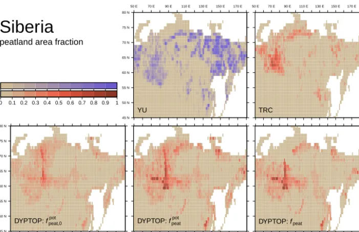
Figure 7. Observed and simulated peatland area fraction. Top row: observed, YU is based on Yu et al. (2010), TRC is based on Tarnocai
et al. (2009). Original YU data delineate grid cells with a significant peatland cover fraction (>5 %). Original binary data on 0.05◦×0.05◦ are regridded to represent the fractional area with significant peatland cover fraction on the 1◦×1◦grid. This information is not directly comparable to other panels and is therefore illustrated with a distinct colour key. Bottom row: simulated,fpeatpotis the potential, hydrologically suitable peatland area fraction after peatland establishment,fpeatis the simulated actual peatland area fraction taking account of the carbon balance criteria.
tion. Figures 8 and 9 illustrate these three steps for the boreal regions of North America and Siberia.
The spatial distribution offpeatpot reflects both the topogra-phy and the soil water balance, suggesting that areas in North America with the highest extent and persistency of flood-ing are located around the Hudson Bay includflood-ing large ar-eas on Baffin Island, across a large area of Quebec around 50◦N, and in south-western Alaska. In Siberia, large fpeatpot
are simulated across the WSL at around 60◦N, the North Siberian Lowland at around 70◦N and 90–110◦E, and along the north-east Siberian coast.
In areas where peatlands are simulated to establish, the mean water table position0is generally lifted upwards and flooding persistency tends to be extended. This increases the simulated potential peatland area fraction to values of around 0.9–1.0 along the southern coast of Hudson Bay (HBL) and 0.5–1.0 in the WSL. Outside areas of significant peatland oc-currence, this mechanism takes no effect and thus separates peat-dominated areas from their surroundings and results in the high spatial heterogeneity found by Tarnocai et al. (2009). Although peatlands are simulated to establish in the Quebec region of 60 to 80◦W, and 50◦N,fpeatdoes not attain values as high as in the HBL. This is ultimately due to the limit to the maximum inundated area set by the choice of CTIminin Eq. (3). In other words, topographical properties do not allow for extensive peatland establishment as in the flat terrain of the HBL.
Another way to display this effect is visualized in Fig. 4 which illustrates the array of ranked inundation fractions for each grid cell (f in Eq. 12) before (left) and after (right) peatland establishment. In the latter case, inundation is ex-tended throughout the season and affects larger area frac-tions. Moreover, this mechanism tends to affect mostly those cells that feature large peatland area fractions also according to Tarnocai et al. (2009) and is thus crucial to predict spatially concentrated peatlands in large flatlands.
Other major peatland regions suggested by Yu et al. (2010) around Great Bear Lake (55–55◦N/120◦W) and in Eastern
Siberia are under-represented by the model mainly due to topographical restrictions (see fpeatpot). However, benchmark maps are not consistent with respect to the extent and pres-ence of peatlands in Eastern Siberia.
At higher latitudes of the tundra regions, peatland growth conditions (ptcrit) are mainly responsible for limiting their es-tablishment. Model predictions are consistent with the maps of Tarnocai et al. (2009) and Yu et al. (2010) in suggesting no significant peatland occurrence beyond a climatical northern frontier where cold temperatures limit plant productivity as illustrated in Fig. 8.
Index
North America
peatland area fraction
0 0.1 0.2 0.3 0.4 0.5 0.6 0.7 0.8 0.9 1 45 N 50 N 55 N 60 N 65 N 70 N 75 N
−170 E −150 E −130 E −110 E −90 E −70 E −50 E
YU
45 N 50 N 55 N 60 N 65 N 70 N 75 N −170 E −150 E −130 E −110 E −90 E −70 E −50 E
TRC
45 N 50 N 55 N 60 N 65 N 70 N 75 N
−170 E −150 E −130 E −110 E −90 E −70 E −50 E DYPTOP: fpeat,0
pot
−170 E −150 E −130 E −110 E −90 E −70 E −50 E DYPTOP: fpeat
pot
45 N 50 N 55 N 60 N 65 N 70 N 75 N
−170 E −150 E −130 E −110 E −90 E −70 E −50 E DYPTOP: fpeat
Figure 8. Observed and simulated peatland area fraction in North America. Top row: observed, YU is based on Yu et al. (2010), TRC is
based on Tarnocai et al. (2009). Original YU data delineate grid cells with a significant peatland cover fraction (>5 %). Original binary data on 0.05◦×0.05◦are regridded to represent the fractional area with significant peatland cover fraction on the 1◦×1◦grid. This information is not directly comparable to other panels and is therefore illustrated with a distinct colour key. Bottom row: simulated,fpeat,0pot is the potential
peatland area fraction, considering hydrological suitability without the peatland-water table position feedback,fpeatpotis the potential peatland area fraction, considering hydrological suitability including the peatland-water table position feedback;fpeatis the simulated actual peatland area fraction, taking account of the peatland establishment criteria (ptcrit) and peat expansion and contraction.
is largely limited by the long-term soil carbon balance. In these regions, the difference between litter inputs (governed by NPP) and decomposition rates (governed by soil temper-ature and moisture) is not sufficiently large to allow for long-term C accumulation in peatland soils. In the remaining ar-eas, LPX simulates suitable conditions for peatland estab-lishment, but their extent is limited by the topographical set-ting and ultimately by the simulated inundation persistency. The global overview of Fig. 10 reveals the dominant role of topography to limit peatlands not only along major moun-tain ranges (e.g. Ural, Rocky Mounmoun-tains), but also in eastern Siberia and Quebec. Smaller areas with long-term C accu-mulation in peatland soils are simulated in the mid-latitudes and the tropics, but these appear to be located mainly in areas where topography and inundation persistency limit peatland extent.
6.3 Peatland carbon
Simulated global C stored in peatland soils is 555 GtC (mean over years 1982–2012), with 460 GtC stored in northern, 88 GtC in tropical, and 8 GtC in southern peatlands. This is broadly compatible with the estimate by Yu et al. (2010) of 547, 50, and 15 GtC for northern, tropical, and southern peat-land C stocks.
Note that C storage in all peatland soils is simulated un-der the assumption that accumulation occurred over 12 kyr
of constant pre-industrial climate and CO2 (see Sect. 5.2). This simplified setup is chosen to assess the capabilities of a dynamic peatland model without having to rely on infor-mation of the climatic past. Therefore, values should not be considered as an explicit estimate for present-day peatland C storage and are thus not highlighted further.
7 Discussion
The TOPMODEL approach presented here provides a cost-efficient solution to the challenge of dynamically simulat-ing the global distribution and the seasonal variation of in-undated areas. We combine this information with simulated C accumulation in persistently inundated soils to predict the spatial distribution of peatlands and its temporal change. 7.1 TOPMODEL implementation
com-parable to flooding data that represent areas where the water table is above the surface. TOPMODEL predictions for the area fraction at maximum soil water should be regarded as a surrogate for the inundation area fraction that should fol-low similar spatial and seasonal patterns and exhibit a similar sensitivity to climate change.
7.1.1 Choice of model parameters
Apart from LPX-specific variables related to the soil water balance, the simulated inundated area fractionf is governed by the function9 and is thus sensitive to the choice of pa-rameters M(in Eq. 2) and CTImin(in Eq. 3). Similarly, the peatland area fractionfpeatdepends not only on LPX’s pre-dictions for the soil C balance, but (in addition to M and CTImin) also on the choice ofNin Eq. (13) andλin Eq. (11) (for a discussion on peatland-specific parameter choice, see Sect. 7.2.2).
Mrepresents a physically based parameter describing the exponential decrease of soil transmissivity with depth (Beven and Kirkby, 1979). Here, we consider M as a tunable but globally uniform parameter. This is in contrast to Ringeval et al. (2012), who modified the CTI values to obtain best re-sults. We tested the model performance in terms of simulated
f for a range of parameter valuesMand CTIminthat yield plausible results for the total simulated inundated area f. Then, given a selected parameter combination (M, CTImin), we assessed a range of parameter values N to simulate the potential peatland area fractionfpeatpot.
Increasing M causes a general contraction in f. Note, however, thatMandf do not relate linearly, but depend on the distribution of CTI. CTImin“caps” the maximum flooded area fraction in each grid cell and thus limitsf in areas with generally low CTI values (mountainous regions). We first constrained CTIminto a range that appears plausible. The ef-fect of varying CTImin within this range (here we assessed CTImin=10, 12, and 14) is rather small for the annual mean total inundated area but slightly affects the seasonal ampli-tude.
ploration of a broader range of parameter value combina-tions partly resolved the apparent differences in spatial het-erogeneity but resulted in a pronounced underestimation of the seasonal variability and an overestimation of total inun-dated area.
7.1.2 Comparison with GIEMS
The model is generally successful at capturing the global dis-tribution of the seasonal maximum inundated area fraction and the seasonal timing of maxima across the globe. Differ-ences in observed and simulated maximum inundation are mainly linked to the spatial pattern and the distribution of values for maximum inundation. While the TOPMODEL ap-proach suggests large areas of extensive inundation with rel-atively low values, the GIEMS data suggest more spatially confined inundation areas and feature areas with high val-ues that are not captured by the TOPMODEL approach. For example, simulated extensive inundation with values around 5–20 % across large areas in the Amazon region, the Tibetan Plateau, or Eastern Siberia appear not to be supported by the GIEMS data. In contrast, high values along rivers (e.g. Amazon, Mississippi, Euphrates, Ganges, Brahmaputra) and in regions containing major or numerous inland water bod-ies (e.g. boreal Canada, Paraná, Pantanal, Lake Chad) are not captured by our TOPMODEL implementation. This apparent disagreement has to be interpreted with regard to the caveats of the GIEMS data set mentioned in Sect. 5.3.1. A simi-lar mismatch between observations and TOPMODEL-based simulation results was found by Ringeval et al. (2014). Ex-tensive inundation is simulated by DYPTOP in areas clas-sified as “Flooded Forest” or “Wetland” in the Global Lakes and Wetlands Database (Lehner and Döll, 2004). Melack and Hess (2010) quantify the “floodable” area fraction of mapped areas within the Amazon basin at 15 %. This agrees well with the seasonal maximum inundated area fraction across the Amazon catchment of 13 % suggested by our results (av-erage over 1992–2004).
and thus excludes permanent water bodies. Consequently, the maximum simulated inundation area fraction is limited to the land area fraction in the respective grid cell, while values in the GIEMS data include permanent water bodies. This con-ceptual difference in the nature of the observational vs. model data contributes to the apparent disagreement in regions with extensive water bodies as mentioned above.
Third, high values of observed annual maximum inunda-tion area in India, around the Mekong river, and in southern and eastern China are due to widespread wet rice agricul-ture with “anthropogenic wetlands” in the form of rice pad-dies. The model applied here does not account for any an-thropogenic land use or land cover change. It is to be noted that these anthropogenic land surface modifications appear to have resulted in a substantial amplification of naturally oc-curring flooding and its seasonal amplitude.
7.1.3 Regional characteristics
While hydrological studies commonly focus on the scale of river basins, inundation is not necessarily confined to an in-dividual basin. We thus investigated six deliberately selected continental-scale regions where each region is characterized by a similar seasonal hydrological regime and contains some of the major global wetlands. Within each region, the model broadly captures the observed range of total inundated area and the timing of seasonality. Simulated areas do not exhibit any consistent bias across regions and model-observation dif-ferences appear to be linked to land cover characteristics in individual regions (e.g. extensive forest cover, or “anthro-pogenic wetlands” as mentioned above).
The model applied here neglects the temporal dynamics of downstream water redistribution within the catchment. In-stead, inundation is driven by the variations in the immediate soil water balance which does not account for delayed ef-fects of preceding runoff. This aspect is likely to contribute to the overestimated rate of inundation retreat after the sea-sonal maximum in areas with large river basins (see SA and AF in Fig. 6). Such a flooding hysteresis has also been dis-covered by Prigent et al. (2007) by comparing precipitation seasonality with inundation seasonality.
In high-latitude regions of North America and Siberia, a similar hysteresis between river discharge and inundation area has been identified by Papa et al. (2008). The model applied here fails to reproduce this pattern, with the sea-sonal maximum inundation being too early and the retreat too quick. The former may be linked to a crude model rep-resentation of snow melt, ice jams in the river valley during early spring (Ringeval et al., 2012), or the fact that inunda-tion is simulated as soon as the uppermost soil layer is no longer frozen, irrespective of remaining snow cover, which would prevent satellites from detecting water. A similar mis-match has been found by Ringeval et al. (2012) in boreal North America. The overestimated rate of retreat may also be related to the structure of different river basins where
dis-connections between the river channel and floodplains may cause delayed inundation retreat but it is not captured by the model (Ringeval et al., 2012).
7.1.4 TOPMODEL in combination with soil moisture models
Model predictions for inundation areas are determined by the simulated soil water balance. However, soil moisture across the soil profile, percolation, and runoff generation are often not physically resolved in vegetation and land surface mod-els. This makes it difficult to evaluate modelled soil mois-ture against observational data, which themselves are subject to notorious caveats (Schumann et al., 2009). In LPX, soil moisture is modelled as an index ranging from 0 at the per-manent wilting point to 1 at field capacity, while water in ex-cess of the field capacity is diverted to runoff. This prevents the soil pore volume from being fully water-filled and hence the water table position from reaching the surface. Yet TOP-MODEL essentially relies on the information of the water ta-ble depth (or deficit to saturation). How can this challenge be met? Here, we define “0” as an index combining soil water content and runoff. This resolves the problem of notoriously low actual water table positions in index-based soil moisture models. Furthermore,0is modified to account for the pres-ence of impermeable frozen soil layers. This leads to a higher susceptibility to flooding in affected regions.
Additionally, we tested to what degree additional informa-tion on the drainage capacity (permeability) of the sub-soil substrate could help to improve simulation results. The new data set on sub-soil permeability by Gleeson et al. (2011) is designed for global applications in land surface/vegetation models. We found that in combination with a soil water bal-ance model of the type implemented in LPX, this additional information does not suit its purpose as soil moisture in the upper layers is hardly affected by drainage from the low-est layer. However, an implementation of this data set may have great potential in combination with a soil water bal-ance model where percolation across soil layers and runoff are simulated based on physical diffusion equations and in-filtration limitation (Ekici et al., 2014).
7.1.5 TOPMODEL as a diagnostic
balance, but the latter may vary most as heterotrophic activ-ity responsible for decomposition is largely inhibited under anoxic conditions, i.e. when soils are waterlogged. However, water saturation/flooding is constrained by the local topo-graphical setting and any prediction of the peatland distribu-tion has to account for this sub-grid scale informadistribu-tion. There-fore, we applied a TOPMODEL implementation to account for soil moisture redistribution within a catchment area and to dynamically determine where inundation is sufficiently persistent for peatland establishment, and combined this with a model for C and water dynamics in peatland soils.
Most previous modelling efforts had to rely on externally prescribed maps defining the peatland distribution based on present-day observations, and available paleoecological syn-theses have relied exclusively on basal dates of existing peat-lands (MacDonald et al., 2006; Yu et al., 2010; Yu, 2011), thus implicitly ruling out the existence of peatlands that have now disappeared. Also the response of peatland extent un-der future scenarios of climate change has been contradictory (Ise et al., 2008; Gignac et al., 1998; Bragazza et al., 2008), partly owing to the unresolved processes of lateral expansion and retreat. Kleinen et al. (2012) have proposed a solution to some of these challenges by combining a TOPMODEL ap-proach with the LPJ-WhyMe model for peatland C and wa-ter dynamics. The DYPTOP model presented here follows the same path and extends the scope by adding the tempo-ral dimension of peatland expansion and retreat in response to changes in climate, CO2 and (potentially) the presence of ice sheets. This opens up a new perspective on the terres-trial C balance over multi-millennial timescales and glacial– interglacial cycles where peatlands may both appear and dis-appear in different regions.
Compared to the model presented by Kleinen et al. (2012), DYPTOP also appears successful at producing the previously unresolved spatial heterogeneity of the global-scale peatland distribution. This is mainly achieved by accounting for the el-evation of the grid-cell-mean water table depth by peatlands and their large water retention capacity. Additional tests (not shown) have also revealed that it is crucial to average CTI values in Eq. (2) over the respective catchment area, and not
eral peatland expansion and contraction. In the approach cho-sen here, peatland area fraction may scale up from the min-imum fraction of 0.001 to 100 % in 1158 yr. This is set by the model parametersfpeatmin, and the relative areal change rate of 1 % yr−1 in Eq. (14). This approach assumes that expan-sion is proportional to the peatland area and implies expo-nential areal growth where the potential peatland area frac-tion is attained on centennial to millennial timescales after initiation (ptcritswitched to TRUE). The choice of these pa-rameters does not significantly affect the results presented here as shifts in the spatial peatland distribution were rel-atively minor throughout the 20th century. Simulated peat-land C storage in grid cells not fulfilling establishment crite-ria (ptcrit=FALSE) is only 2.9 TgC (0.0005 % of the global simulated peat C at 1900 (570 PgC)) and is therefore negli-gible for global C budgets. Further studies could be aimed at assessing these temporal dynamics by benchmarking DYP-TOP driven by transiently changing climate and CO2since the Last Glacial Maximum. Peatland initiation could be used as a target variable and compared to observational data on basal ages (MacDonald et al., 2006).
7.2.2 Choice of model parameters
We assessed the simulated peatland area fraction and total C storage for a range of DYPTOP model parametersN (see Eq. 13),λ(see Eq. 11),Cpeat∗ , anddC
∗ peat
dt (see Fig. 3) and
com-pared results with data from Yu et al. (2010) and Tarnocai et al. (2009). Increasing N reducesfpeatpot and vice versa. λ
affects0mineraland increasing values reducefpeatpot in regions affected by permafrost (most effectively in east Siberian bo-real regions). This can be assessed offline, asfpeatpot repre-sents the potential peatland area fraction before peatland es-tablishment and depends only onf =9(0mineral). However, the simulated actual peatland area fraction is subject to the effects of peatland establishment and an offline optimiza-tion to constrain parameters is not possible. Furthermore, the simulated peatland soil C pools and therefore (indirectly)