A Variable Structural Control for a Flexible Plate

(1)

A New Fuzzy Regression Model by Mixing Fuzzy and Crisp Inputs

Magda M. M. Haggag

1

Abstract

This paper proposes a new form of the multiple regression model (mixed model) based on adding both fuzzy and crisp input data. The least squares approach of the proposed multiple regression parameters are derived in different cases. This derivation is based on the fact that each fuzzy datum is a nonempty compact interval of the real line. The main contribution is to mix both fuzzy and crisp predictors in the linear regression model. The mixed fuzzy crisp model will be introduced mathematically and by coded via R-language. The least squares of the regression parameters will be derived and evaluated using distance measures. Numerical examples using generated data showed best results for the mixed fuzzy crisp multiple regression models compared to the multiple fuzzy models.

Keywords: Bertolouzza distance, Compact data sets, Euclidean distance, Fuzzy least squares, Fuzzy variables, Fuzzy regression, tight data.

(1) Introduction

Linear regression models are used to model the functional relationship between the response and the predictors linearly. This relationship is used for describing and estimating the response variable from predictor variables. Some important assumptions are needed to build a relationship, such as existing enough data, the validity of the linear assumption, the exactness of the relationship, and the existence of a crisp data for variables and coefficients. The fuzzy regression model is a practical alternative if the linear regression model does not fulfill the above assumptions. A fuzzy linear regression model first introduced by Tanaka et al. (1982). Their approach handled after that by many authors, such as Tanaka and Lee (1988); Tanaka and Watada (1988); Tanaka et al. (1989); Diamond (1988, 1990, 1992); Diamond and Koener (1997); D’Urso and Gastaldi (2000); Yang and Lin (2002); D’Urso (2003); Gonzalez-Rodriguez et al. (2009); Choi and Yoon (2010); Yoon and Choi (2009, 2013); D’Urso and Massari (2013).

Fuzzy regression models have been treated from different points of view depending upon the type of input and output data. There are three different kinds of models:

 Crisp input and fuzzy output with fuzzy coefficients.  Fuzzy input and fuzzy output with crisp coefficients.  Fuzzy input and fuzzy output with fuzzy coefficients.

The least squares method is used to estimate the fuzzy regression model. (See for instance, Diamond (1988, 1990, 1992)).

The objective of this paper is to extend the simple linear regression model to the multiple one and estimate it with the least squares approach. This extension is based on adding both fuzzy and crisp predictors to the linear regression model, and the resulting model is called the mixed fuzzy crisp (MFC).

1_{Associate Professor of Statistics, Head of the Department of Statistics, Mathematics, and Insurance, Faculty of Commerce,}

(2)

Our extended model will be evaluated using the extended squared distance of Diamond (1988). Generated data are applied to compare the estimation results of the proposed MFC model with the usual multiple fuzzy MF regression model.

This paper will be outlined as follows. Section (2) presents some definition regarding fuzzy random variables (FRVs), fuzzy distance and possibility distributions will be introduced. In section (3) fuzzy linear regression models will be considered. The proposed mixed fuzzy and crisp (MFC) linear regression model will be introduced in section (4). Section (5) considers the numerical applications using generated and real data examples. The concluding remarks will be discussed in section (6).

(2) Mathematical Preliminaries

Some definitions and notes will be presented in this section for the requirements of this work. 2.1 Sets Representation of Fuzzy Numbers

Let

 

p c R

K denotes the class of all non-empty compact intervals of p

R

and let

 

p c R

F denotes the class of all fuzzy numbers of p

R

. Then,

 

p c R

F will be defined as follows:

 

p 



: p 

 

0,1| _ _c

 

p 





 

0,1



,

c R A R A K R

F (1)

where

A

 is the α-cut set of A if







0 ,

1 

, and A0 is called the support of A. (Zadeh, 1975).

For a given A,BF_c

 

R , and

b



R

, the followings hold:

The sum of A and B is called the Minkowski sum, defined as: S ABF_c

 

R . (Zadeh, 1975). The scalar product of b and the set A is defined as: PbAF_c

 

R . (Zadeh, 1975).

A fuzzy number DF_c

 

R is called the Hukuhara difference of A and B defined as:

D



A



_H

B

, it is shown that the Hukuhara difference is the inverse operation of addition



, where

A



B



D

.(Zadeh, 1975).

2.2 Left and Right (L-R) Representation of Fuzzy Numbers

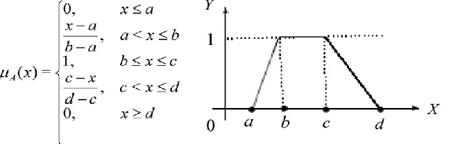
Let A∈T(R) is a FRV, where T(R) is a set of trapezoidal fuzzy numbers of Fc(R). A trapezoidal fuzzy number A is

defined as A=Tra(Al,Au,Av,Ar), where Al∈R and Ar∈R arethe left and right limits of the trapezoidal fuzzy number A,

respectively. AlsoAu∈R and Av∈R arethe left and right middle points of A, respectively, as shown in Figure (1). When

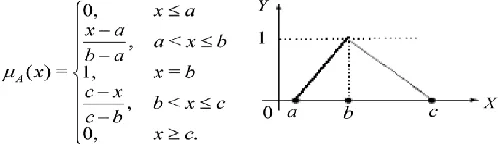
Au = Av =Am, a fuzzy number A will be a triangular, i.e., A=Tri(Al,Am,Ar), as shown in Figure (2)

If Al=a, Au=b,Av=c,and Ar=d, a stylized representation of a trapezoidal fuzzy number A can be represented in

the following L-R form:

A trapezoidal fuzzy number A is specified by a shape function with the following membership (Figure (1)):

(3)

When c=b, a triangular fuzzy number A is specified by a shape function with the following membership (Figure (2)):

Figure (2): Triangular Fuzzy Number 2.3 Metrics in Fuzzy Numbers Space

To measure the distance between any two fuzzy numbers A, and B in

F

_c

 

R

, an extended version of the Euclidean (L2) distance (

d

_E



A

,

B



) is defined by:







_



 



 





_

1



 



 



0

2 1

0

2 2

,

B

A



B



d



A



B



d



A

d

_E _L _L _U _U , (4)

where

A

L

 



and AU

 



are the lower and upper



-cuts of a fuzzy number A. (Grzegorzewski, 1998 ).

Bertoluzza et al. (1995) have proposed the so-called Bertoluzza metric d(A,B), which is defined as:







_

_{ }



 



 





_

_{ }



 



 



1 , 0

2 1

, 0

2 2

,

B

mid

A

_

mid

B

_

d



spr

A

_

spr

B

_

d



A

d

, (5)

where

 

2

L U

A

mid

_







 denotes the midpoint of

A

, and

 

2

L U

A

spr

_







 denotes the spread (or radius) of

A

,







 

0 ,

1

. AUand AL denote the upper bound and lower bound of A, respectively.

The Hausdroff

d

_H



A

,

B



metric for A,BFc

 

R is given by:



A

,

B



max



inf

A

inf

B

,

sup

A

sup

B



,

d

_H





(6)

where infA is the infimum value of A, and supA is the supremum value of A. The d_p



A,B



metric for A,BF_c

 

R , and 1 pis given by:





sup

,

2

1 inf

inf

2

1 ,

1

p p p

p

A

B

A

B

A

B

d













_

_

_



(7).

where infA and supA are the infimum and supremum values of A, respectively. (See Vitale, 1985).

The distance between fuzzy numbers can be defined as the distance between their membership functions. The distance dp



A,B



between the two fuzzy numbers A,B is given by:









p

X

p

B A

p A B dm

d

1

, 









, for 1 p, (8)

and



A B



essential

 

x

 

x

d A B

X x

p ,  _ sup







for p, (9)

where X 



is a Lebesgue measurable set, m is a Lebesgue measure on X. (See Klir and Yuan, 1995).

(4)



A B



 

x

 

x x



X E



dp , 0



A 



B    ,

If the two functions d1and d2 defined such that:

d1 and d2 : XFXF R,

where XF is a fuzzy set and X={x1,x2,…,xn} is a fuzzy random variable (FRV), and

A

,

B



X

F.

Then:





_

 





 n

i

i B i

A x x

B A d

1

1 ,



, (10)

and





_



 







 n

i

i B i

A x x

B A d

1

2

2 ,



, (11)

Are called fuzzy distances. (Rudin, 1984).

The FRVs used in this paper are considered as functions from a probability space (Ω,A,P) into the metric space (Fc(R),dθ), where θ>0. The sample mean Xn and sample variance

2 ,n





of the FRV X are defined by:



n



n X X X

n

X 1 1 2... , (12)

and



i n



n

i

n d X X

n ,

1

1 2 2

,





 





. (13)

If X and Y are two FRVs , then the Bertoluzza covariance between them is defined as:



X,Y



covmid



X,Y



covspr



X,Y



cov  



, (14)







_

_{ }

_



 



 

 



_

_{ }



 



 

 

 0,1

1 , 0

1

1 ,

cov mid X _ mid Y _ d



mid X _ mid Y _ d



n Y

X _i _i _n _n

n

i

mid (15)







_

_{ }

_



 





 





_

_{ }



 



 

 

 0,1

1 , 0

1

1 ,

cov mid X _ mid Y _ d



mid X _ mid Y _ d



n Y

X i i n n

n

i mid

(3) Fuzzy Linear Regression Models

3.1 The Standard Linear Regression Models

Consider the following standard simple linear regression model:

i i

i X

Y 



₀



₁ 



, i=1,2,…,n, (16)

where



0, and



1 are unknown parameters, X is the predictor, Y is the response variable and



is the error

term of the model, with

E





\

X





0

and finite variance. The least squares estimators of



0, and



1are obtained by

minimizing the sum of squared error criterion, Q, as follows:









 

 n

i

i X

Y Q

1

2 1 1 0 , ₁

0

min

arg



 . (17)

(5)





2 1

2 1 1

x

n

x

y

x

n

y

x

b

_n

i i n

i i i









 _, _and_b _y _b_x

1

0   . (18)

The multiple linear regression model is one:







 X

Y , (19)

where Y is an (n×1) column vector of the dependent variable, X is an (n×p) matrix of predictors, β is a (p×1) vector of unknown parameters to be estimated, and ε is an (n×1) vector of errors distributed as N(0,σ2_I_n_{). The least}

squares estimator of β , denoted by b is given by:



XX



XY

b  1  , (20)

which is obtained by minimizing the corresponding criterion, Q as:





 





 Y X Y X

Qargmin    . (21)

3.2 Simple Fuzzy Linear Regression Models

In the case of using fuzzy data, fuzzy regression models will be used to estimate the unknown parameters. Consider the following fuzzy simple linear regression models:





~ ~

~

1 0 

 i

i x

y , (22)





~

1 0





_i

i

x

y

, (23)





~

1 0





_i

i

x

y

, (24)

where



0

,

and



1, are crisp parameters,

x

is a crisp variable, 0 1

~

,

~



and

are fuzzy parameters, ~yis a fuzzy

response variable,

~

x

is a fuzzy predictor. As a lack of linearity of

 

p c R

F ,



~

is reduced to a non-FRV. (See

Gonzalez-Rodriguez et al. (2009)).

The regression functions of models (22), (23), and (24) will be approximated as follows:

X

Y

E

(

~

\

~

)





₀





₁

~

, (25)

X

Y

E

(

~

\

)





~

₀





~

₁ , (26)

X

Y

E

(

~

\

~

)





~

₀





~

₁

~

, (27)

The least squares estimators of the parameters in models (22):(24) are derived using using triangular and trapezoidal fuzzy numbers. The derivation is approximated by optimizing the least squares criterion. In this work, the least squares optimization criterion which is an extension version of that introduced by Diamond (1988) will be used. 3.3 The least Squares Approach for of the Simple Fuzzy Regression Models Using Triangular Fuzzy Numbers

The least squares estimators of the parameters in model (22) are obtained by minimizing the least squares criterion as follows:





_









 n

i

i x

y d Q

1

1 0 2 ,

1

0, argmin ~, ~

1 0



 (28)

Diamond (1988) showed that there are two cases arising when 0

1 



or 0

1 



. Using the triangular fuzzy number, the objective function in (28), when 0

1 

(6)











 









              n i ir ir im im il il n i i i x y x y x y x y d Q 1 2 1 0 2 1 0 2 1 0 , 1 1 0 2 , 1 0 1 0 1 0 min arg ~ , ~ min arg ,



    (29)

By differentiating of Eq. (29) with respect to the parameters



₁and



0, and equating the equations by zero:





_

_

_

_

_

_

0

2

2 ,

1 1 1 0 1 1 1 1 0 1 1 1 1 0 1 1 1

0











    n i r i ir r i n i m i im m i n i l i il l

i

y

x

y

x

y

x

Q

_







_

_

_

_

_

_

0

2

2 ,

1 1 1 0 1 1 1 0 1 1 1 0 0 1

0











    n i r i ir n i m i im n i l i

il

x

y

x

y

x

y

Q

_



The least squares estimators,

b

1 and



0

b of



₁and



0 respectively, are obtained as follows:











  











_n i ir im il n i ir ir im im il il

x

n

x

y

x

n

y

x

y

x

y

x

b

1 2 2 2 2 1 1

3

, (30)

x b y

b₀   ₁ , (31)

where, yil , yim , and yir are the left, middle, and right value of yi , respectively, for i=1,2,…,n. Also, xil , xim , and

xir are the left, middle, and right value of xi , respectively, for i=1,2,…,n. y



y y y



n

i

ir im

il /3

1





 

 , and



x x x



n

x

n

i

ir im

il /3

1



    .

For the second case, where 0

1 



, the objective function of (28) will be as follows:











 









              n i il ir im im ir il n i i i x y x y x y x y d Q 1 2 1 0 2 1 0 2 1 0 , 1 1 0 2 , 1 0 1 0 1 0 min arg ~ , ~ min arg ,



   

, (32)

and differentiating of Eq. (32), the least squares estimators,

b

1 and



0

b of



₁and



0 respectively, are

obtained as follows:











  











_n i ir im il n i ir ir im im il il

x

n

x

y

x

n

y

x

y

x

y

x

b

1 2 2 2 2 1 1

3

, (33)

b₀  yb₁x. (34)

Diamond (1988 [5], 1990[6]) showed that for every fuzzy nondegenerate data set that

b

1



b

1 , and the least

(7)

Definition (3.1)

Consider the fuzzy data sets yi



yil,yim,yir



~ _ _{, and}





ir im il

i x x x

x , ,

~ _ _{, for i=1,2,…,n, the set is said to be} nondegenerated, if not all observations in a set are made at the same datum.

Definition (3.2)

Consider the fuzzy data sets yi



yil,yim,yir



~ _ _{, and}





ir im il

i x x x

x , ,

~ _ _{, for i=1,2,…,n, the set is said to be} tight if either

b

₁



0

or

b

₁



0

. If

b

₁



0

the data set is said to be tight positive, and if

b

₁



0

the data set is said to be tight negative. (Diamond (1988[5]).

The least squares estimators of the parameters in model (23) are obtained by minimizing the squared distances between the regression model and the regression function as follows:





_





   n i i i x y d Q 1 1 0 2 , 1 0 ~ ~ , ~ min arg ~ , ~ 1 0



  (35)

where



~

₀







₀_l

,



₀_m

,



₀_r



and



~

₁







₁_l

,



₁_m

,



₁_r



are two triangular fuzzy numbers. Eq. (35) can be written as:

 









 



2



1 0 2 1 0 2 1 0 , 1 1 0 2 , 1 0 1 0 1 0 min arg ~ ~ , ~ min arg ~ , ~ i r r ir i m m im i l l il n i i

i x y x y x y x

y d

Q



              



 (36)



₁l,



₁m,



₁r and



0l,



0m,



0r, the least

squares estimators,

b

1l,

b

1m,

b

1rand b0l, b0m,

b

0r are obtained when

x

i≥ 0 as follows:





 



 





_n i i n i l il i l

x

n

x

y

x

n

y

x

b

1 2 2 1 1 ,





 



 





_n i i n i m im i m

x

n

x

y

x

n

y

x

b

1 2 2 1 1 ,





 



 





_n i i n i r ir i r

x

n

x

y

x

n

y

x

b

1 2 2 1

1 , (37)

x

b

y

b

₀_l



_l



₁_l ,

b

₀_l



y

_l



b

₁_l

x

, .

b

₀_r



y

_r



b

₁_r

x

. (38) when

x

i< 0 , least squares estimators,

b

1l,

b

1m,

b

1rand b0l, b0m,

b

0r are obtained as follows:





 



 





_n i i n i r ir i l

x

n

x

y

x

n

y

x

b

1 2 2 1 1 ,





 



 





_n i i n i m im i m

x

n

x

y

x

n

y

x

b

1 2 2 1 1 ,





 



 





_n i i n i l il i r

x

n

x

y

x

n

y

x

b

1 2 2 1

1 , (37)

x b y

b₀_l  _l ₁_r , b₀_m y_mb₁_mx , b₀_r y_r b₁_lx. (38)

The least squares estimators of the parameters in model (24) are obtained by minimizing the squared distances between the regression model and the regression function as follows:





_





   n i i i x y d Q 1 1 0 2 , 1 0 ~ ~ ~ , ~ min arg ~ , ~ 1 0



 (39)

where 0



0l

,

0m

,

0r



~

_





, 1



1l

,

1m

,

1r



~

_





, and

~

x

i





x

il

,

x

im

,

x

ir



are triangular fuzzy numbers, and

i

x

~

1 0



(8)

 









 



2



1 0 2 1 0 2 1 0 , 1 1 0 2 , 1 0 1 0 1 0 min arg ~ ~ , ~ min arg ~ , ~ ir r r ir im m m im il l l il n i i

i x y x y x y x

y d

Q



              



 (40)



1l,



1m,



1r and



0l,



0m,



0r, the least

squares estimators,

b

1l,

b

1m,

b

1rand b0l, b0m,

b

0r are obtained as follows when xi's

~ _and

1

~



are positive fuzzy numbers.





 



 





_n i l il n i l l il il l

x

n

x

y

x

n

y

x

b

1 2 2 1 1 ,





 



 





_n i m im n i m m im il m

x

n

x

y

x

n

y

x

b

1 2 2 1 1 ,





 



 





_n i r ir n i r r ir ir r

x

n

x

y

x

n

y

x

b

1 2 2 1

1 , (41)

l r l

l

y

b

x

b

₀





₁ ,

b

0m



y

m



b

1m

x

m , b0r  yr b1lxr. (42)

The derivation of the fuzzy simple least squares estimators using trapezoidal fuzzy numbers can be easily found. 3.4 Multivariate Fuzzy Linear Regression Models

3.4.1 Multivariate Fuzzy Linear Regression Models for Fuzzy Predictors and Crisp Parameters

Consider the case of fuzzy simple linear regression models defined in (22), the multiple fuzzy regression model may be formalized as follows:

i ip p i

i

i x x x

y



~



~ ...



~



~ ~

2 2 1 1

0     

 . (43)

Suppose using centered values of fuzzy predictors, Eq. (43) can be written in matrix form as follows:





~

~_ _

X

Y , (44)

where, Y~ is an (n×1) vector , X~ is an (n×p) matrix of p fuzzy predictors, and



is a (p×1) vector of unknown p crisp parameters. As a result of the lack of linearity of

 

p

c R

F ,



~

is reduced to a non-FRV



. (See Gonzalez-Rodriguez et al. (2009)).

Y~, X~,



, and



are formalized in matrix form as follows:















n

y

Y

~

2 1



,















   p n n n p p

x

X

~

2 1 2 22 21 1 12 11











,















p





2 1 , and















n



~

2 1



,

where yi



yil,yim,yir



~ _ _{, and}





ijr ijm ijl

ij x x x

x , ,

~ _ _{, for i=1,2,…,n, and j=1,2,…,p.}

The least squares estimator of β in model (44), for triangular fuzzy variables, can be formalized as follows:



X

l



X

l



X

m



X

m



X

r



X

r





X

l



Y

l



X

m



Y

m



X

r



Y

r





1

ˆ



, (45)

where,



ijl j



l x x

X   , Xm 



xijmxj



, Xr 



xijr xj



, are (n×p) left, middle, and right fuzzy matrices of

predictors. Yl 



y1l,y2l,...,ynl



, Ym 



y1m,y2m,...,ynm



, Yr 



y1r,y2r,...,ynr



, are (n×1) response vectors

such that: p ipl l i l i

il x x x

y  ₁



₁ ₂



₂...



, for i=1,2,…,n

p ipm m i m i

im x x x

(9)

p ipr r

i r i

ir x x x

y  ₁



₁ ₂



₂...



, for i=1,2,…,n

The least squares estimator of β in model (44), for trapezoidal fuzzy variables, can be formalized as follows:



X

l



X

l



X

u



X

u



X



X



X

r



X

r





X

l



Y

l



X

u



Y

u



X



Y



X

r



Y

r







  





ˆ

1

, (46)

where,



ijl j



l x x

X   , Xu 



xiju xj



, X 



xij xj



,Xr 



xijr xj



, are (n×p) left, middle left, middle

right, and right fuzzy matrices of predictors. Yl 



y1l,y2l,...,ynl



, Yu 



y1u,y2u,...,ynu



,



  



 y y yn

Y  ₁ , ₂ ,..., , Yr 



y1r,y2r,...,ynr



, are (n×1) response vectors such that: p

ipl l

i l i

il x x x

y  ₁



₁ ₂



₂...



, for i=1,2,…,n

p ipu u

i u i

iu x x x

y  ₁



₁ ₂



₂ ...



, for i=1,2,…,n

p ip i

i

i x x x

y  1



1 2



2... 



for i=1,2,…,n p

ipr r

i r i

ir x x x

y  1



1 2



2...



, for i=1,2,…,n

3.4.2 Multivariate Fuzzy Linear Regression Models for Crisp Predictors and Fuzzy Parameters

Consider the case of fuzzy simple linear regression models defined in (23), the multiple fuzzy regression model can be generalized as follows:

i ip p i

i

x

y





~





~





~



...





~





~

2 2 1 1

0 . (333)

Suppose using centered values of crisp predictors, Eq. (43) can be written in matrix form as follows:







 ~

~

X

Y , (44)

where, Y~ is an (n×1) fuzzy vector , X is an (n×p) matrix of p crisp predictors, and



~ is a (p×1) vector of unknown p fuzzy parameters. As a result of the lack of linearity of

 

p

c R

F ,



~



. (See

Y~, X ,



~, and

















n

y

Y

~

2 1



,















  

p n n

n

p p

x

X











2 1

2 22

21

1 12

11

,

    

 

    

 



p



~ ~ ~

~ 2

1

 , and















n





2 1

,

where yi



yil,yim,yir



~ _ _{, and}





jr jm jl

j



~



,

, for i=1,2,…,n, and j=1,2,…,p.

The least squares estimator



ˆ of



~in model (44), for triangular fuzzy variables, can be formalized as follows:





l



m



r





ˆ

_

ˆ

_,

ˆ

_,

ˆ

_,

where,





 

l l



X



X



Y

1

ˆ



, (45)







m



m



X



X



Y

1

ˆ



,





 

r r



X



X



Y

1

ˆ



,

(10)



xij xj



X   , and Yl 



y1l,y2l,...,ynl



, Ym 



y1m,y2m,...,ynm



, Yr 



y1r,y2r,...,ynr



, are (n×1)

response vectors such that:

pl ip l

i l i

il x x x

y  1



1  2



2 ...



, for i=1,2,…,n

pm ip m

i m i

im x x x

y  1



1  2



2 ...



, for i=1,2,…,n

pr ip r

i r i

ir x x x

y  ₁



₁  ₂



₂ ...



, for i=1,2,…,n

The least squares estimator of



~in model (44), for trapezoidal fuzzy variables, can be formalized as follows:





l



u



v



r





ˆ

_

ˆ

_,

ˆ

_,

ˆ

_,

ˆ

_,

where,





 

l l



X



X



Y

1

ˆ



,





 

u u



X



X



Y

1

ˆ



,





 

v m



X



X



Y

1

ˆ







 

r r



X



X



Y

1

ˆ



.

3.4.3 Multivariate Fuzzy Linear Regression Models for Fuzzy Predictors and Fuzzy Parameters

Consider the case of fuzzy simple linear regression models defined in (24), the multiple fuzzy regression model can be generalized as follows:

i ip p i

i

x

y





~





~





~



...





~





~

2 2 1 1

0 .

Suppose using centered values of crisp predictors, Eq. (43) can be written in matrix form as follows:







 ~~

~

X

Y , (44)

where, Y~ is an (n×1) fuzzy vector , X~ is an (n×p) matrix of p fuzzy predictors, and



~ is a (p×1) vector of unknown p fuzzy parameters. As a result of the lack of linearity of

 

p

c R

F ,



~



. (See

Y~, X~,



~, and

















n

y

Y

~

2 1



,















  

p n n

n

p p

x

X

~

2 1

2 22

21

1 12

11











,

    

 

    

 



p



~ ~ ~

~ 2

1

 , and















n





2 1

,

where yi



yil,yim,yir



~ _ _,





ijr ijm ijl

ij x x x

x , ,

~ _ _and





jr jm jl

j



~



,

, for i=1,2,…,n, and j=1,2,…,p. The least squares estimator



ˆ of



~in model (44), for triangular fuzzy variables, can be formalized as follows:





l



m



r





ˆ

_

ˆ

_,

ˆ

_,

ˆ

_,

where,



l l





l l



l



X



X



Y

1

ˆ



, (45)



m m





m m



m



X



X



Y

1

ˆ



,



r r





r r



r  XX XY 1

ˆ



,

(11)



ijl j



l x x

X   , Xm 



xijmxj



, Xr 



xijr xj



, are (n×p) left, middle, and right fuzzy matrices of

predictors.Yl 



y1l,y2l,...,ynl



, Ym 



y1m,y2m,...,ynm



, Yr 



y1r,y2r,...,ynr



, are (n×1) response vectors

such that:

pl ipl l

l i l l i

il x x x

y  1



1  2



2 ...



, for i=1,2,…,n

pm ipm m

m i m m i

im x x x

y  ₁



₁  ₂



₂ ...



, for i=1,2,…,n

pr ipr r

r i r r i

ir x x x

y  ₁



₁  ₂



₂ ...



, for i=1,2,…,n

The least squares estimator of



~in model (44), for trapezoidal fuzzy variables, can be formalized as follows:



ˆ

_l





X

_l



X

_l



1



X

_l



Y

_l



,

u





X

u



X

u





X

u



Y

u



1

ˆ



,



v v





v v



v



X



X



Y

1

ˆ



r 



XrXr





XrYr



1

ˆ



.

(4) The Proposed Mixed Fuzzy Crisp (MFC) Regression Model

All the fuzzy multiple regression models that have been considered in the literature handled the cases where all the predictors are fuzzy or all are crisp.

In this section, a new multiple linear regression model which mixes the fuzzy and crisp predictors in one model called “Mixed Fuzzy Crisp” (MFC) regression model, is proposed.The least squares approach for the new model is derived based on positive tight data as defined in (3.2) and triangular fuzzy numbers. Also, the properties of the resulting regression parameters are introduced in two cases: first, when the parameters are fuzzy, and second when the parameters are crisp.

4.1 The Proposed Mixed Fuzzy Crisp (MFC) Regression Model Using Crisp Parameters

Consider the case where the multiple linear regression model concludes some fuzzy and some crisp predictors. The computations will be done using triangular fuzzy number, and can applied to trapezoidal one. Assuming centered predictors, the proposed simplest form of multiple model that contain two predictors, one is crisp and the other is fuzzy, with crisp parameters will be as follows:

i i i

i x x

y 



1~1



2 2 



~ _. ₍₄₇₎

where yi



yil,yim,yir



~ _ _{, and}





r i m i l i

i x x x

x₁ ₁, ₁ , ₁

~ _ _{, for i=1,2,…,n,}





im im im

i x x x

x₂  , , , and



i is a non-fuzzy

error with mean equal zero. The regression function of model (47) will be as follows:

E

(

~

y

\

~

x

₁

,

x

₂

)





₁

~

x

₁





₂

x

₂.

The derivation of the least squares estimators is done by minimizing the squared distances between the regression model and the regression function as follows:

























_











_

_

_

_

_













 



 

n

i

n

i

i r i ir i

m i im n

i

i l i il

n

i

i i

i n

i

i i

i

x

y

x

y

x

y

x

y

x

y

d

Q

1 1

2 2 1 1 1 2

2 2 1 1 1

2 2 1 1 1 ,

1

2 2 2 1 1 ,

1

2 2 1 1 2 ,

2 1

~

min

arg

~

,

~

min

arg

~

,

~

min

arg

,

1 0

1 0 1

0



 

  



(48)



₁, and



2, the following equations are

(12)

  _ _ _ _ _ _ 0 2 2 2 , 1 1 2 2 1 1 1 2 2 1 1 1 1 2 2 1 1 1 1 1

0          

 

_

    n i n i i r i ir r i i m i im m i n i i l i il l

i y x x x y x x x y x x

x

Q _ _ _ _ _ _

  





1



1 1 2 2



1



1 1 2 2



0

1

2 2 1 1

1         





 i m im im i ir ir ir i

n i i l i il l

x





        









n i n i n i ir r i im m i il l i n i n i r i r i n i n i m i m i n i n i l i l

i

x

y

x

y

x

y

x

1 1 1

1 1 1 1 1 2 1 2 2 1 1 1 1 2 1 2 2 1 1 1 1 2 1 2 2 1

1







_



                _ _     n i n i n i ir r i im m i il l i n i n i n i n i r i m i l i r i m i l

i x x x x x x x x x y x y x y

x

1 1 1

1 1

1

1 1 1 1

2 1 2 1 2 1 2 2 1 2 1 2 1 1 

 , (49)

and,





_

_

_

_

_

_

0 2 2 2 , 1 1 2 2 1 1 2 2 2 1 1 2 1 2 2 1 1 2 2 1

0          

 

_

    n i n i i r i ir i i m i im i n i i l i il

x

Q

_















0

1 1 2 2 1 1 2 2 2 1 1 2 1 2 2 1 1

2         





   n i n i i r i ir i i m i im i n i i l i il

x





              n i ir i n i im i n i il i n i n i n i i i r i i m i n i i l

i x x x x x x x y x y x y

x 1 2 1 2 1 2

1 1 1

2 2 2 2 1 1 2 1 1 1 2 1

1



3



. (50)

Solving the equations (49) and (50), the least squares estimators,



ˆ

₁, and



ˆ

₂, of



₁, and



₂are obtained respectively, as follows:





 





 



   











_n i n i i ir im il n i i n i ir r i im m i il l i

x

y

x

y

x

y

x

y

x

1 1 2 2 1 2 2 2 1 2 1 1 1 1 1 1

3

3 ˆ



, (51)









 



  









_n i i n i n i ir im il ir r i im m i il l i

x

y

x

y

x

y

x

1 2 1 1 1 2 2 2 1 1 1 1 2

ˆ



, (52)

where, yil , yim , and yir are the left, middle, and right value of yi , respectively, for i=1,2,…,n. Also, xi1l , xi1m ,

and xi1r are the left, middle, and right i’s value of

~

x

₁ , respectively, for i=1,2,…,n.





_



     n i i n i i ir i im i

ilx y x y x x

y y 1 2 1 2 2

2 / , and









     n i i n i ir im

il x x x

x x

1 2 1

1 / are the weighted means of ~y and

1

~

_x

_{, respectively, using the observations of the crisp predictor} 2

x

as weights. All the above results can be shown for trapezoidal fuzzy data.