6XUIDFH5HFRQVWUXFWLRQIURP3DUWLDOO\6WUXFWXUHG
1RLV\&ORXGRI3RLQWV8VLQJ%6SOLQHV
5DLPXQGDV/LXWNHYLþLXV$QGULXV'DYLGVRQDV
Department of Systems Analysis, Vytautas Magnus University Vileikos st. 8, LT – 44404, Kaunas Lithuania
e-mail: [email protected], [email protected]
http://dx.doi.org/10.5755/j01.itc.42.1.1391
$EVWUDFW. This paper presents a new approach how to reconstruct a parametric surface from a partially structured and noisy cloud of points representing surface that has a centre-line, such that all perpendicular rays to that line intersects with a surface not more than once. Presented algorithm analyses partially structured cloud of points, generated by point based 3D scanner and calculates parameters to build a non-uniform B-spline 3D mesh.
.H\ZRUGV3D surface reconstruction; Non-uniform B-spline; Parametric surfaces; 3D scanning and visualization; Point cloud approximation.
,QWURGXFWLRQ
Digital 3D models are widely used in scientific data visualization, entertainment industry, orthotics and prosthetics (medicine), quality control and inspection, industrial design, documentation of cultural artefacts and many other areas. There are many techniques to create digital 3D models and one of those techniques is a 3D model generation from a cloud of points, acquired from 3D scanners. An output of a point based digital 3D scanner is a set of surface coordinates that are used as a raw data either for a further pre-processing or a direct synthesis of a 3D model. To generate a 3D geometric model from a cloud of points most often triangulation algorithms like Cocone or Crust are used because of their ability to process unstructured cloud of points (acquired coordinates from a 3D scanner) [12]. The triangulation methods work well when the cloud of points is dense enough and is not noisy, because a surface is reconstructed by combining neighbour points into triangles. The quality of the result surface very much depends on the distance between and the position of the points in a cloud. Another important thing to note about the triangulation algorithms is that additional data pre-processing, like triangle mesh simplification or refinement, smoothing, reorientation of faces, filling of the holes and other repairs is usually needed in order to increase the quality and decrease complexity of the reconstructed surface.
An alternative to triangulation algorithms are algorithms that use parametric curves for the
reconstruction of a surface from coordinates. Such algorithms gained attention for several advantages: parametric surfaces are the exact analytical representations, have the potential of the three dimensional shape editing, parametric models require less data to describe an object, have easily adjustable level of detail (LOD), and are convertible to triangulated one, but not vice versa [14].
This paper presents an algorithm for creating a parametric surface from a partially structured and noisy cloud of points. An algorithm calculates coefficients of a non-uniform B-spline surface, i.e. fits a B-spline surface to a cloud of points.
6RXUFHGDWDDQGGHILQLWLRQV
In this paper a cloud of points that represents a surface of an object is acquired using an experimental 3D scanner [10]. This 3D scanner rotates an object in small steps and measures a distance to its surface at different levels (see Figure 1).
Measured data are stored in a cylindrical coordinate system representation and are converted to the Cartesian space during a pre-processing step. Conversion is required, because linear interpolation, approximation, filtration of flat surface areas in cylindrical coordinate system would cause undesired curvature (arcs, etc.) on the final surface. Also data may be acquired in Cartesian coordinate system if other 3D scanners are used.
All points in the same level have common coordinate zand form a layer. Distribution of points in the same layer and between layers can be arbitrary.
A presented algorithm is capable of reconstructing a 3D surface, which has a centre-line, such that all perpendicular rays coming out from that line intersect with the surface not more than once.
Surface points are defined for a scanned surface as:
च,൫ݔ,,ݕ,,ݖ,൯, (1)
ݖ,=ݖ,ାଵ, 1 ݆ ߚ, 1 ݅ ߛ .
Here x,y, and zrepresent point’s coordinates in the Cartesian coordinate system, ɀ is a number of layers and ȕi is a number of points in a single layer i.
In this paper a presented algorithm converts a cloud of points into a parametric non-uniform B-spline surface that is defined as:
ࡼ(ݑ,ݒ) =σ௦ୀσௗୀ௧ ࡺ,(ݑ)ࡺௗ,(ݒ)ࡼ,ௗ (2)
ݑ ݑ ݑାଵ,ݒ ݒ ݒାଵ.
Here p is a surface degree in u direction; q is a surface degree in v direction; ࢁ= { ݑ|0 ݇ ݏ+
+ 1} is a B-spline’s knot vector in u direction;
ࢂ= {ݒ|0 ݈ ݐ+ݍ+ 1} is a B-spline’s knot
vector in v direction; ࡺ,(ݑ) and ࡺௗ,(ݒ) are B-spline’s blending functions of degree p and q,
respectively; Pc,d are B-spline’s control (de-Boor) points; u and vare parametrization intervals (infinite set of points in a predefined range) and should not be confused with single values. The parameters U, V,
ࡺ,(ݑ), ࡺௗ,(ݒ)and Pc,dare described in more detail in the following sections.
5HSUHVHQWDWLRQRISDUWLDOO\VWUXFWXUHGFORXG
RISRLQWVLQWRDSDUDPHWULFVXUIDFH
2YHUYLHZRIDQDOJRULWKP
This paper describes a new approach how to compute unknown parameters U,V,ࡺ,(ݑ), ࡺௗ,(ݒ) and ࡼ,ௗ of a parametric B-spline surface P(u,v), described in (2) so that it approximates a cloud of points च.
Calculating parameters for a B-Spline surface equation directly from a cloud of points is a difficult task. In order to perform this task, knot vectors for a surface have to be defined. It appears that in a generated data cloud there are no two perpendicular
directions for which selected knot values could meet Shoenberg-Whitney conditions [13]. Those conditions are necessary and sufficient for the approximation of cloud of points with a B-spline to be possible.
To overcome the problem, an approach to split a cloud of points into several slices was proposed, implemented and results presented to demonstrate its advantage over the known algorithms.
In the presented approach a cloud of points is split into three different matrices X,Y, and Z, where each corresponding entry in matrices contains a corresponding coordinate of a point. These matrices then are used as a data source to calculate B-Spline parameters for each coordinate separately from equations:
ࡼ(௫)(ݑ,ݒ) =σ σ ࡺ
,(ݑ)ࡺௗ,(ݒ)ࡼ,ௗ
(௫) ௧
ௗୀ ௦
ୀ (3)
ࡼ(௬)(ݑ,ݒ) =σ σ ࡺ,(ݑ)ࡺௗ,(ݒ)ࡼ,ௗ
(௬)
௧ ௗୀ ௦
ୀ (4)
ݑ ݑ ݑାଵ,ݒ ݒ ݒାଵ.
B-Spline parameters for Z coordinate values are derived from the already calculated parameters, as described in Subsection 3.5.
A process to calculate unknown parameters of equations (3) and (4) is divided into four steps that are explained in details in the next subsections (see Figure 2).
)LJXUH. The process of parametric surface creation The first step is a pre-processing step where input data are converted from cylindrical to Cartesian coordinate system. Then, during the second step, knot vectors Uand V have to be defined. This is done by subdividing pre-processed data into estimated number of segments towards two perpendicular directions u
used to create corresponding knot vectors U and V. During the third step B-spline blending functions
ࡺ,(ݑ)andࡺௗ,(ݒ)are calculated from knot vectors and data projections in uand vdirections, using Cox-deBoor recurrence [5]. In the last, forth step, B-spline control points Pc,d are calculated based on blending functions and other calculated data by applying optimization in the least square sense.
When parameters for equations (3) and (4) are calculated, they are combined to form parameters for a parametric surface (2) that approximates input dataच. Then a parametric surface can be displayed or saved for the further use.
3UHSURFHVVLQJRILQSXWGDWD
Experimental 3D scanner stores acquired points in the cylindrical coordinate system [10]. Pre-processing step is necessary to convert those points into the Cartesian representation.
Experimental 3D scanner, used for data acquisition, operates in a non-ideal environment; it has specific mechanical characteristics, limited accuracy and is affected by electrical noise. As a result, at different levels measurements might occur at different positions and if the measurements are stored in a matrix Cas given below in (5), the matrix will most likely contain some number of empty elements rij[10].
To decrease the size of the matrix C, acquired data in columns are quantized into 8000 intervals in a range of (0° - 360°) with a step size equal to 0,045°. Step size value here is a smallest detectable step size of a stepper motor, converted into angle and divided by 2. The number of rows in the matrix C depends on the number of stops a laser sensor makes in a vertical direction (Figure 1). A distance between layers in this case varied in a range [1,25-1,55] mm. An absolute vertical position of a layer is stored in a first column of the matrix C. The structure of the matrix Cis:
=
ۉ ۈ ۈ ۈ ۇ
0 ߠଵ ߠଶ … ߠ … ߠ
߬ଵ ݎଵ,ଵ ݎଵ,ଶ … ݎଵ, … ݎଵ,
߬ଶ ݎଶ,ଵ ݎଶ,ଶ … ݎଶ, … ݎଶ,
ڭ ڭ ڭ ڰ ڭ ڰ ڭ
߬ ݎ,ଵ ݎ,ଶ … ݎ, … ݎ,
ڭ ڭ ڭ ڰ ڭ ڰ ڭ
߬ ݎ,ଵ ݎ,ଶ … ݎ, … ݎ,ی
ۋ ۋ ۋ ۊ
(5)
here ߠ,ݎ,߬are angle, radius and height respectively, m
is the number of layers and n is the number of quantization intervals in every layer i (Figure 3).
)LJXUH. Relationship between cylindrical and Cartesian
coordinate systems
A conversion from the cylindrical to the Cartesian coordinate system is straightforward:
ቐ
ݔ,=ݎ,× cosߠ,
ݕ,=ݎ,× sinߠ ,
ݖ,=߬.
(6)
After the conversion, object’s surface is represented by ݉×݊ number of points, including empty ones. Conversion results are stored in three separate matrices X, Y and Z, where each row corresponds to a layer data in a cloud of points:
ࢄ= (ݔ,),ࢅ= (ݕ,),ࢆ= (ݖ,) (7)
ݖ,=ݖ,ାଵ, 1 ݅ ݉, 1 ݆ ݊.
MatricesX,Yand Zare sparse because matrix (5) consists of empty entries.
The sparseness is the most undesirable property of a data set and needs to be corrected to proceed. The problem can be solved by inserting data into sparse areas using, for example interpolation between neighbor data points. If the input data contains a considerable amount of noise, it is recommended to apply data filtering before performing data correction. Otherwise noise can lead to undesirable deformations on the reconstructed surface. Recommendations on the selection of filters can be found in [4].
Data sparseness can be eliminated using a linear interpolation algorithm. In this paper a slightly modified algorithm was used:
SURFHGXUHinterpolate(X,Y,ș)
// in: X – x coordinates of surface points // in: Y – y coordinates of surface points // in: ș – position angle from matrix (5) // out: X,Y
EHJLQ
IRUeach row iin matrix XGR
=index of last non empty element in row i; ݎ =index of first non empty element in row i; IRUeach column jin matrix XGR
LIࢄ,is not empty WKHQ p=j;
r=index of next non empty element in row i; LIris empty WKHQ
r= index of first non empty element in row i; HQGLI
HOVH
LIߠ> ߠWKHQݍ=ߠെ360; HOVHݍ=ߠ;HQGLI
LIߠ> ߠWKHQݍ݆=ߠെ360; HOVHݍ݆=ߠ;HQGLI
݇=ିఏ ೝି;
ࢄ,=ࢄ,× (1െ ݇) +ࢄ,×݇;
ࢅ,=ࢅ,× (1െ ݇) +ࢅ,×݇;
Further steps in the algorithm will be performed with pre-processed matrices Xand Y.
&DOFXODWLRQRINQRWYHFWRUV
A B-spline surface is defined by a set of curves that intersect and form surface patches. To create such a structure, matrices XandY are subdivided into estimated number of segments: rnumber of segments in a row direction u and w number of segments in a column direction v(Figure 4).
)LJXUH. Segmentation of matrices. The same schema is
used to create segments in matrices Xand Y
These segments are called B-spline local segments or knot intervals. The number of segments and the number of data points in them depend on input data distribution in coordinate space and a degree of a surface in both directions uand v. In B-spline theory, a cubic spline is the most common type, sufficient to approximate most types of shapes, so cubic B-spline surface i.e. of order 4 (degree = 3) is used through this paper too.
Input data spacing in row direction u is directly related to z coordinate of each data layer. To maintain this information and use it in calculations, a vector H
is defined as:
ࡴ= (݄ଵ,݄ଶ, … ,݄, … ,݄) = (ݖଵ,ଵ,ݖଶ,ଵ, … ,ݖ,ଵ). (8) To represent input data spacing in column direction va vector Ais defined as:
=൫ܽଵ,ܽଶ, … ,ܽ, … ,ܽ൯= (1,2, … ,݊). (9) Because data points in v direction were interpolated using linear interpolation, spacing of points is considered to be uniform and is encoded as a sequence 1,2,...,n in the vector A. Segments of B-splines are estimated from the vectors Hand Arather than values in matrices Xand Y.
Segments have to be selected according to the following requirements:
ݑ ݄ ݑାଵ,
1 ݅ ݉, 0 ݇ ݎ, 1 ݎ ݉ െ , (10)
ݒ ܽ ݒାଵ,
1 ݆ ݊, 0 ݈ ݓ, 1 ݓ ݊ െ ݍ. (11)
Here r and w are numbers of segments in directions u and v, respectively; p and q are B-spline degrees in directions uand v, respectively; ݑand ݒ are B-spline knots, which match with position values of segment endpoints in corresponding directions u
and v. These requirements ensure that Shoenberg-Whitney conditions are met i.e. it is possible to create a valid parametric surface that approximates a given data set [13].
The number of segments r and w depends on a priori knowledge about the input data and the desired approximation properties, and should be selected individually. A common methodology on how to select
rand wwas not developed as it was not a scope of this research. In an ideal case, a quantity of segments in each direction should be selected so that curves of selected degrees p and q are flexible enough to accurately approximate data that fall into successive segments. In practice, there should be at least one segment defined in each direction, but usually the number of segments should be greater than one in order to create a good surface approximation. On the other hand, if too many data points fall into a single segment, smoothing effect arise and a final surface might be distorted. If noise presents in input data, smoothing effect might be desired and it can be controlled by changing the number and the size of segments. In this paper 100 segments were chosen in the row direction uand 100 segments - in the column direction vin order to define knot vectors.
Knots ݑand ݒin corresponding directions u and
v can be calculated using predefined functions as segmentation templates and selected depending on variation of values in vectors A and H. Examples of such functions can be a linear function, a Gaussian function, or other. If distances between values in vectors Aand Hare random, a use of linear function is suggested. In the presented algorithm a linear function was used to define knots (see algorithm calcKnots below).
Knot vectors U and V are created from knots ݑ
and ݒ. In order to force B-spline curves to begin at the first control point and to end at the last control point, knot vectors were modified by duplicating the first and the last knots pand qtimes, respectively. As a result, the knot vector Uis:
ࢁ= (ݑ, … ,ݑ,ݑଵ,ݑଶ, … ,ݑିଵ,ݑ, … ,ݑ) (12) and vector Vis:
SURFHGXUHcalcKnots(H,A,r,w,p,q) // in: H – see equation (8)
// in: A – see equation (9)
// in: r – number of segments in udirection // in: w – number of segments in vdirection // out: U,V – knot vectors
EHJLQ
m= length(H);
IRUi= 0 to (r+ 2 × p)GR LIi<pWKHQ
Ui+1=H1;
HOVHLIi>r+p – 2WKHQ Ui+1=Hm;
HOVH
Ui+1=H1+ (i - p) × (Hm – H1) / m – 1;
HQGLI HQGIRU n= length(A);
IRUj= 0 to (w+ 2 × q)GR LIj<pWKHQ
Vj+1=A1;
HOVHLIj>w+q – 2WKHQ Vj+1=An;
HOVH
Vj+1=A1+ (j - q)× (Am – A1) / n – 1;
HQGLI HQGIRU HQG
The same knot vectors are used to approximate data in both matrices Xand Y.
&DOFXODWLRQRI%VSOLQHEOHQGLQJIXQFWLRQV
B-spline’s are constructed using basis functions, which are blended together and transformed by control points in order to achieve a desired shape. These functions are named blending functions and according to (2)-(4) are encoded in parameters ࡺ,(ݑ) and
ࡺௗ,(ݒ) . At this point relation between parametrization intervals uand vin expressions (3)-(4) and values hi and aj in expressions (10)-(11) can be
noticed. As a result, blending functions can be calculated using parameters݄א ݑ, and ܽא ݒand be denoted as ࡺ,(݄)andࡺௗ,(ܽ).
B-spline blending functions ࡺ,(݄)andࡺௗ,(ܽ) are defined by p+1 and q+1 non-zero coefficients respectively. Coefficients must be selected to satisfy the following requirements:
ࡺ,(݄)0, ࡺௗ,(ܽ)0,
σ௦ୀࡺ,(݄) = 1, σ௧ௗୀࡺௗ,൫ܽ൯= 1, (14)
ݑ ݄ ݑାଵ,1 ݅ ݉,
ݒ ܽ ݒାଵ, 1 ݆ ݊.
Here ࢁ= {ݑ|0 ݇ ݏ++ 1} and
ࢂ= {ݒ|0 ݈ ݐ+ݍ+ 1} are B-spline’s knot
vectors.
Coefficients of blending functions ࡺ,(݄) and
ࡺௗ,൫ܽ൯in this paper are calculated using Cox-de Boor recurrences [5]:
Initialise ࡺ,(݄) =൜1,0, otherwise ݄א ൣݑ,ݑାଵ൯,
ࡺௗ,൫ܽ൯=൜1,0, otherwise ܽא ൣݒ,ݒାଵ൯,
ࡺ,(݄) = (݄െ ݑ)
ࡺ,ିଵ(݄)
ݑାെ ݑ
+
+൫ݑାାଵെ ݄൯ ࡺାଵ,ିଵ(݄) ݑାାଵെ ݑାଵ,
(15)
ࡺௗ,൫ܽ൯=൫ܽെ ݒ൯
ࡺௗ,ିଵ൫ܽ൯
ݒାെ ݒ
+
+൫ݒାାଵെ ܽ൯ࡺௗାଵ,ିଵ൫ܽ൯ ݒାାଵെ ݒାଵ .
(16)
The same two sets of parameters ࡺ,(݄) and
ࡺௗ,(ܽ)are used to approximate data in matrices X and Y, because the knot vectors U, V and the parameters in vectors H,Afor both matrices are also the same. Matrices Xand Yare defined in (7).
&DOFXODWLRQRI%VSOLQHFRQWUROSRLQWV
The shape of B-spline surface P(u,v) is formed using control (de-Boor) points ࡼ,ௗand blending functions ࡺ,(ݑ)and ࡺௗ,(ݒ), equation (2). Control points normally do not belong to B-Spline surface, but this property depends on knot vectors. In the proposed algorithm knot vectors are designed so that the control points at the edges of a surface match with the surface points.
As knot vectors and blending functions are calculated using parameters݄א ݑ,ܽ א ݒ, equation (2) can be expressed as:
ࡼ൫݄,ܽ൯=σ௦ୀσௗୀ௧ ࡺ,(݄)ࡺௗ,൫ܽ൯ࡼ,ௗ, (17)
ݑ ݄ ݑାଵ,ݒ ܽ ݒାଵ,
1 ݅ ݉, 1 ݆ ݊.
Here ࢁ= {ݑ|0 ݇ ݏ++ 1} and ࢂ=
{ݒ|0 ݈ ݐ+ݍ+ 1}are B-spline knot vectors.
Since ࡺ,(ݑ) in (17) does not depend on the index d, the equation can be rewritten as:
ࡼ൫݄,ܽ൯=σ௦ୀࡺ,(݄)൫σ௧ௗୀࡺௗ,൫ܽ൯ࡼ,ௗ൯.(18)
Then inner sum can be denoted as ࡽ,:
ࡼ൫݄,ܽ൯=σ௦ୀࡺ,(݄)ࡽ,, (19)
ࡽ,=σ௧ௗୀࡺௗ,൫ܽ൯ࡼ,ௗ. (20)
ߜଶ= minொ,ೕσ หࡰ,െ ࡺ,ࡽ,ห ଶ
ୀଵ , (21)
ࡺ,=൮
ܰଵ,ଵ ܰଵ,ଶ ڮ ܰଵ,௦
ܰଶ,ଵ ܰଶ,ଶ ڮ ܰଶ,௦
ڭ ڭ ڰ ڭ
ܰ,ଵ ܰ,ଶ ڮ ܰ,௦
൲,
ࡽ,=
ۉ ۇ
ܳଵ,
ܳଶ,
ڭ
ܳ௦,ی
ۊ,ࡰ,=
ۉ ۇ
ܦଵ,
ܦଶ,
ڭ
ܦ,ی
ۊ,
0 ܿ ݏ, 1 ݆ ݊.
Here |ή| is the length of vector, ࡰ, stores the acquired data coordinates Xor Y.
Equation (20) hides sover-determined systems of linear equations with s×t unknown coefficientsࡼ,ௗ. Assuming that the parameters ࡺௗ,൫ܽ൯are stored in the matrix ࡺ,ௗ, the unknown coefficients can be calculated by minimizing a sum:
߮ଶ= min,σ หࡽ, ் െ ࡺ
,ௗࡼ்,ௗห ଶ
ୀଵ , (22)
ࡺ,ௗ=൮
ܰଵ,ଵ ܰଵ,ଶ ڮ ܰଵ,௧
ܰଶ,ଵ ܰଶ,ଶ ڮ ܰଶ,௧
ڭ ڭ ڰ ڭ
ܰ,ଵ ܰ,ଶ ڮ ܰ,௧
൲,
ࡼ,ௗ=൮
ܲଵ,
ܲଶ,
ڭ ܲ௧,
൲
்
,ࡽ,=൮
ܦଵ,
ܦଶ,
ڭ ܦ,
൲
்
,
0 ܿ ݏ, 0 ݀ ݐ.
All over-determined systems of linear equations can be solved separately using least squares or other algorithms.
Expressions in equations (21) and (22) are minimized twice: the first time – to find control points
ࡼ(௫,ௗ)and to approximate the data in the matrix X, and the second time – to find control points ࡼ,ௗ
(௬)
and to approximate the data in matrix Y. Both matrices are defined in (7).
In the experiments described in this paper, a minimization problem is solved using QR decomposition. In case of large input data (over 200 000 points), Householder transformations are used to perform QR decomposition [7].
A final parametric surface P(u,v) will contain c×d
control points:
ࡼ,ௗ=ቀࡼ,ௗ
(௫),ࡼ ,ௗ
(௬),ࡼ ,ௗ
(௭)ቁ, (23)
0 ܿ ݏ, 0 ݀ ݐ.
The third component ࡼ(௭,ௗ)can be calculated using the following equation:
ࡼ(௭,ௗ)=൫ࢁశభାڮାࢁశ൯
. (24)
Here Uis the knot vector in u direction, and p is the degree of a surface in udirection.
6WRULQJSDUDPHWULFVXUIDFH
In order to restore a parametric surface it is enough to store the values of two knot vectors in both uand v
directions (Section 3.3) and control points ࡼ,ௗ (Section 3.5). Most of the 3D APIs accept those parameters in their surface reconstruction functions.
As an alternative, control points ࡼ,ௗand sets of parameters ࡺ,(ݑ) and ࡺௗ,(ݒ) can be saved (Section 3.4). Then there would not be necessary to recalculate coefficients of blending functions when loading a surface from a hard disk drive, but this approach has several disadvantages: 1) it takes at least 3 times more storage space on a hard disk drive; 2) collocation matrices are usually not accepted in well-known 3D API’s, such as OpenGL, etc., and 3) GPU based visualisation of a parametric surface, including generation of collocation matrices from knot’s, is usually done faster than providing already predefined collocation matrices so saving of parameters of blending functions does not add any value.
STEP, IGES and others file formats can be considered for saving and describing parametric surface in more standardized way. Although today’s CAD system’s have their own methods for representing and exchanging data. As a result data representation and exchange issues may arise. Some recommendations how to minimize bad consequences of the data exchange using STEP is provided in [11].
,PSOHPHQWDWLRQ
The presented surface reconstruction algorithm is part of the 3D surface reconstruction system (see Figure 5).
systems of linear equations has to be solved. MATLAB implementation of QR algorithm was used (function qr) for this task. qr function in Matlab uses the LAPACK [9] routines DGEQP3, DORMQR and DTRTRS (see MATLAB documentation). The presented surface reconstruction algorithm calculates B-spline surface parameters and outputs them into a text file. This file then is used as an input data in the visualization step. Model visualization part was implemented using C# language and Tao Framework - OpenGL wrapper for .NET.
([SHULPHQWDOUHVXOWV
For the experiments a statue (Figure 6 (a)) was scanned using a point based laser scanner [10]. As a result, a set of 144 450 data points in 136 layers was acquired and saved in a sparse data matrix (5). This set of points was used as input data for testing different surface reconstruction algorithms. The result of the presented surface reconstruction algorithm is shown in Figure 6 (g-h) and was compared to the neighbour triangulation algorithm (f) described in [4] and the other three well known 3D surface reconstruction
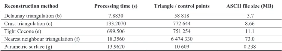
algorithms: Delaunay, Crust and Tight Cocone, Figure 6 (b-e). The performance and other statistical results were also compared and provided in a Table 1.
The processing time in Table 1 includes average time required to read the data, to calculate 3D surface and to save the results on storage disk using a PC with 2.4GHz Core 2 Duo CPU and 4GB memory. 3D surface was visualized using OpenGL library and hardware accelerated graphics enabled. Triangulation results were stored in a plain text object file format (OFF). This has to be taken into account when comparing sizes of output file presented in Table 1.
Figure 6b shows a result of simple Delaunay triangulation algorithm. This algorithm gave the worst visual result. Data points in a resulting data structure were not connected correctly and a large number of triangles were positioned incorrectly too. A triangle mesh was created using CGAL implementation of Delaunay triangulation [2] and a natural neighbor approach.
Figures 6c and 6d show the results of the Crust triangulation algorithm [1]. The algorithm does a
a) b) c) d)
e) f) g) h)
)LJXUH. Results of surface reconstruction algorithms: (a) a test object – 18,2 cm height statue , (b) Delaunay triangulation [2], (c) Crust triangulation [1], (d) Crust triangulation with surface correction, (e) Tight Cocone triangulation [6] with surface
7DEOHExperimental statistics of methods for surface reconstruction (average values)
5HFRQVWUXFWLRQPHWKRG 3URFHVVLQJWLPHV 7ULDQJOHFRQWUROSRLQWV $6&,,ILOHVL]H0%
Delaunay triangulation (b) 7.8830 58 818 3.7
Crust triangulation (c) 133.2070 772 644 8.66
Tight Cocone (e) 699.506 751 254 11.1
Nearest neighbour triangulation (f) 18.3560 6 474 330 73.0
Parametric surface (g) 13.9620 10 609 0.238
manifold extraction in order to form a regular surface and uses a ball pivoting method to extract a manifold and to return outward’s normal’s orientation. Because of the noise and uneven distribution of the input data, the resulting surface is not water-tight (there are holes on the surface), have errors in manifold structure and the orientation of faces. Surface after reorientation of triangle faces is shown in figure 6d. The errors are best seen at the bottom part and near the ear on the head of the statue. Also, small noise covers the entire surface. The performance of the algorithm is the worst if compared to the other analyzed algorithms.
Figure 6e shows the result of the Tight Cocone algorithm. The algorithm is based on the cocone algorithm that uses a single Voronoi/Delaunay computation. It is supposed to be water-tight and is claimed to be scale and density independent [6]. In this algorithm, the number of holes is reduced by stitching them from existing Delaunay triangles and without inserting new points. The result is similar to the one produced by the Crust algorithm: the surface is not water-tight, has errors in the manifold structure and the orientation of faces. The algorithm was tested with several parameters. Only the best achieved result (after performing face reorientation) is presented in figure 6e. The Tight Cocone triangulation algorithm takes about 50 times more time and about 46 times more storage space for a surface reconstruction than using our parametric reconstruction algorithm (see Table 1). The code for the Tight Cocone, released for academic use, can be downloaded from [3].
Figure 6f shows a result of simple nearest neighbour triangulation algorithm that creates tight triangulated surface and can be used to perform real time triangulation with partial data. The algorithm is based on RBF, triangle strips and predictable structure of cloud of points [4]. The algorithm gives better results than the previous triangulation algorithms. The recreated surface is water-tight and without noticable errors, processing time is relatively small. However, the algorithm creates a large number of triangles. This might be a problem to render and manipulate such a reconstructed surface. Also, the generated output is not very smooth if compared to the presented algorithm.
The result of the algorithm, presented in this paper, (Figure 6g) is constructed from cubic non-uniform B-spline curves that lay down horizontally and vertically as shown in Figure 6h. The surface contains 100 B-spline segments in each directions and the total
of 103x103=10609 control points. 150 approximation steps in each direction in B-spline surface were made to draw the surface displayed in Figure 6g and 80 steps - for the surface in Figure 6h. The generated surface is watertight (without surface holes) and smooth compared to the results of the previously analyzed algorithms. Our algorithm needs less processing time to calculate surface’s parameters than the Crust and the Tight Cocone algorithms and uses much less storage space to store output results than the analyzed triangulation algorithms (Table 1).
In order to evaluate an approximation accuracy of the presented algorithm in this experiment, vectors connecting input data points and corresponding points on the B-spline surface were calculated. The mean of vector lengths is 0.1377 mm, the standard deviation is 0.2385 mm. These numbers are influenced by the noise and measurement errors that are present in the input data and are filtered out in the B-spline surface.
&RQFOXVLRQV
Experimental results presented in this paper show that the proposed algorithm can be successfully used for the reconstruction of complex geometric surfaces from a partially structured cloud of points that does not fit into a data grid. The algorithm combines well-known parametric and optimisation algorithms with the coordinate-wise surface generation approach to create a non-uniform B-spline surface that can be described with 15 times less data if compared to triangulation surfaces.
The proposed strategy to split input data into separate groups by coordinates and process separately was shown to be working and can lead to expected results.
It was demonstrated that QR decomposition and Householder reflection algorithms can be effectively used for the calculation B-spline surface parameters. Linear interpolation, used in the pre-processing step to adjust input data is shown to be sufficient to solve points-to-surface problem when the input data set is unorganized. This technique simplifies the process of surface subdivision. It also provides information about the distribution of surface points.
)XUWKHUUHVHDUFK
The presented algorithm is targeted to the reconstruction of surfaces, which have a centre-line such that all perpendicular rays to that line intersect with the surface not more than once. In general, it is possible to use the algorithm with the other types of objects. In that case, an object should be subdivided into parts, which satisfy Shoenberg-Whitney conditions [13]. Then parts of the object should be parameterised separately and joined together to form a final surface. The join can be performed using a direct degree elevation of NURBS curves [8] and an integration of curve segments.
In the presented algorithm a linear subdivision of acquired data into segments is used, but possibly better results could be achieved by performing density analysis of the cloud of points and adjusting segments accordingly.
$FNQRZOHGJPHQWV
7KHDXWKRUVZRXOGOLNHWRWKDQN7RPDV.ULODYLþLXV
and Kazimieras Padvelskis from Vytautas Magnus University for their valuable remarks and suggestions, and Tamal K. Dey from the department of CIS at Ohio State University for providing implementation of Tight Cocone algorithm.
5HIHUHQFHV
[1] 1$PHQWD 0%HUQ 0.DPY\VVHOLV. A New
Voronoi-Based Surface Reconstruction Algorithm. In: SIGGRAPH 98, pp. 415-421.
[2] CGAL-Computational Geometry Algorithms Library, 2011. Available at: http://www.cgal.org/.
[3] COCONECocone Software for surface reconstruction and medial axisAvailable at: http://www.cse.ohio-state.edu/~tamaldey/cocone.html
[4] $'DYLGVRQDV 5/LXWNHYLþLXV A PLC Application for Data Scanning and Visualization. In: Proceedings of International Conference “Electrical and Control Technologies–2008”, Kaunas, 2008, pp. 144-149. [5] &GH%RRUOn calculating with B-splines. In: Journal
of Approximation Theory, 6, 1972, pp. 50–62.
[6] 7. 'H\ 6*RVZDPLTight Cocone: A water tight surface reconstructor. In: Proceedings of 8th ACM Symposium. Solid Modeling Appl.,2003, pp. 127-134. [7] *+*ROXE &)9DQ /RDQ Matrix Computations
(3rd ed.), Johns Hopkins University Press, 1996.
[8] .-DQNDXVNDV '5XEOLDXVNDV Direct degree elevation of NURBS curves. In: Information Technology and Control, 2010, Vol. 39, No. 4, pp. 269-283.
[9] LAPACK–Linear Algebra Package. Version 3.3.1, 2011. Available at: http://www.netlib.org/lapack.
[10]5/LXWNHYLþLXV $ 'DYLGVRQDV Positioning of stepper motors in graphical data acquisition system. In: Proceedings of International Conference “Electrical and Control Technologies – 2009”, Kaunas, 2009, pp. 70-74.
[11]* /LXWNXV $ 5LãNXV $ 7RPNHYLþLXV
$/HQNHYLþLXVIssues with exchange of presentation data among CAD systems. In: Information Technology and Control, 2012, Vol. 41, pp. 385-391.
[12]90DWXNDV 03DXOLQDV $8ãLQVNDV
5$GDãNHYLþLXV 50HãNDXVNDV '$ 9DOLQþLXV Survey of Point Cloud Reconstruction Methods. In: Proceedings of International Conference “Electrical and Control Technologies – 2008”, Kaunas, 2008, pp. 150-153.
[13]-6FKRHQEHUJ $:KLWQH\ On Pólya frequency functions. III. The positivity of translation determinants with an application to the interpolation problem by spline curves. Transactions of the American Mathematical Society, 1953, Vol. 74, pp. 246-259.
[14]$:DWW 3D Computer Graphics. Third Edition. Addison-Wesley Publishing, 2000.