Application of Wireless Sensor in Automatic Device

Application of Wireless Sensor in Automatic Device

Baolin Su!!_{", Quanyu Zhang, Boyang Zhang}

Suihua University, Heilongjiang, China [email protected]

Abstract—To improve the cost and accuracy in the positioning method of wireless sensor network in automatic devices, we proposed an improved dis-tance based positioning method. We analyzed the positioning algorithm based on RSSI, TOA, TDOA, AOA distance measure. Due to different geographic shape, the right trajectory is important to the algorithm. We replaced hyperbola curve with asymptote in this study because the hyperbola positioning algorithm is not energy efficiency. We designed the positioning process of asymptote line algorithm. For the computational complexity, the hyperbola asymptotes are judged by the intersection point, which has an additional step compared to the maximum likelihood method. However, the maximum likelihood method must calculate the quadratic equations. The simulation results show that the algo-rithm proposed in this study is better than maximum likelihood method in posi-tioning accuracy and the two algorithms have the same computational complex-city. The process of positioning presented in this study is simple and has a low cost.

Keywords—wireless sensor, mobile anchor node, asymptotic line

1

Introduction

Wireless sensor network is a network composed of a large number of cheap wire-less sensor nodes. It is a kind of computer network composed of many automatic network device randomly distributed in space. These devices use sensors to coopera-tively monitor the environment situation or physical information of different loca-tions, such as temperature, humidity, smell, sound, vibration, pressure, motion or pollutants [1]. The development of wireless sensor network originated in battlefield monitoring and military applications. But now it is used in many fields, such as envi-ronmental and ecological monitoring, health monitoring, home automation, bio medi-cal, emergency rescue and disaster relief, remote control of hazardous area, traffic control and so on [2]. It is a hot research field in the world, which involves many disciplines, high cross and highly integrated knowledge. These applications cannot be separated from positioning technology as the support.

2

State of art

The positioning method of wireless sensor network is divided into range based and range free positioning methods. In distance based positioning, distance measurement methods include TOA, TDOA, and RSSI, and the method to measure the angle con-tains AOA [4]. In consequence, the positioning method based on distance can be divided into: TOA based positioning, TDOA based positioning, RSSI based position-ing and AOA based positionposition-ing[4].

TOA based positioning. In the wireless sensor network, the model of the ultrasonic ranging is that each anchor node installs an ultrasonic generating device, and ordinary nodes are mounted an ultrasonic receiving device. The anchor node transmits ultra-sonic time around and also sends a radio frequency signal. When the ultraultra-sonic wave is emitted, the RF signal sends its transmit time and anchor node position information. In the use of distance measurement, it is necessary to ensure strict time synchroniza-tion, and at the same time, the ultrasonic will be affected by NLOS (non line of sight) propagation. Although the positioning precision based on the positioning algorithm has higher requirements, the nodes maintain strict clock synchronization [5]. The degree of precision of the equipment has a very high demand, and the cost of posi-tioning is high, so it is rarely used at present.

TDOA based positioning. In the positioning mechanism based on the time differ-ence (TDOA), the anchor nodes simultaneously transmit ultrasonic signals and radio frequency signal. When the unknown node receives the radio frequency signal, it is recorded at the time of T1, and when the ultrasonic signal is received, the current time is recorded as T2. This algorithm also requires additional hardware equipment to produce ultrasonic signal and radio frequency signal[6]. But its implementation is easy and it has high positioning accuracy. T1 and T2 are the time recorded for un-known nodes, and (T2-T1) is the absolute time difference of the two signals, which will not make influence because of asynchrony time between nodes. As a result, TDOA range has no strict requirement of time synchronization. However, the ultra-sonic will decay strongly with the increase of distance, so the nodes need to be dense-ly distributed, otherwise the ultrasonic cannot complete the ranging task.

RSSI based positioning algorithm. The RSSI is to transmit at a specific power at the transmitter, and the received power is measured at the receiver. The distance measurement method is obtained based on the comparison between the power loss and the existing empirical model curves. Because the sensor nodes have wireless communication capabilities, this method does not require the aid of additional equip-ment for ranging. The ranging cost is low, but because the actual application envi-ronment is more complex, NLOS, multipath propagation and other issues will have a certain impact on the power loss [6]. Therefore, the use of RSSI ranging, compared with TOA, TDOA has a large range error, which is suitable for the environment has not high requirements of the positioning precision.

measurement angle are complex, it requires greater power consumption. Thus, it is rarely used in sensor network positioning.

Compare the above four algorithms, RSSI does not require additional hardware fa-cilities to support the ranging, cost and complexity is low, and the positioning accura-cy is not high. TDOA, compared with TOA, does not require strict time synchroniza-tion, which is more desirable. While the positioning based on AOA needs complex hardware, so the usually used ranging methods are RSSI and TDOA.

3

Distance based positioning method for wireless sensor

networks

3.1 Mathematical model of hyperbola asymptote positioning based on distance

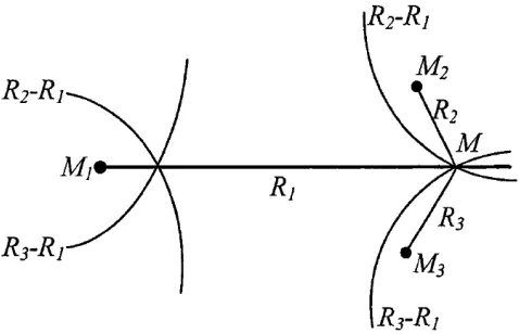
The propagation time of the ultrasonic signal between the unknown node and the moving anchor node is t, and the distance between the unknown node and the anchor node is Ri=vti, i=1, 2, 3..., in which v represents the speed of ultrasonic propagation.

It is known that the distance difference between the anchor node M1 and anchor node

M2 to the unknown node is R21=R2-R1, the unknown node must be located in the

hy-perbola curve with the anchor nodes M1 and M2 as the focuses and the distance

differ-ence to the two focuses of R21. While the distance difference from the anchor nodes

M1 and M2 to the unknown node is R31=R3-R1, it can be determined that the unknown

node is located in the hyperbola curve with the anchor nodes M1 and M2 as the

focus-es, and two focal distance difference of R31. This intersection of the two curves is the

mark of unknown node. Because hyperbola curve has symmetry, the intersection point is two, which requires the adoption of a priori conditions to determine the cor-rect coordinates of the unknown nodes. For instance, it can be judged by the distance measurement. The hyperbola position is shown in figure 1.

The relationship between the unknown node (x, y) and anchor node (xi, yi) in

hy-perbola positioning is:

(x

!

x

)

+

(y

!

y

)

!

(x

!

x

)

+

(y

!

y

)

=

R

(x

!

x

)

+

(y

!

y

)

!

(x

!

x

)

+

(y

!

y

)

=

R

"

#

$

%$

(1)

The equations (1) are nonlinear equations, and R1i is the difference of propagation

distance between the unknown node to the mobile anchor node position 1 and the mobile anchor node position i, and the distance from the unknown node to the posi-tion of the mobile anchor node i is:

R

=

R

+

R

R

=

(R

+

R

)

=

x

+

y

!

2xx

!

2yy

+

x

+

y

When i=1, we can get:

R

+

2

R

R

=

x

+

y

!

2

xx

!

2

yy

!

x

!

y

Here xi1 and yi1 are represented as xi-x1 and yi-y1, respectively. According to (4), it

can be sen that if R1 is regarded as a unknown number, then the equation can be

con-sidered as the equation about x, y and R1, which is conductive to solve the equations.

According to equation (4), we can get a set of equations. When solving the equa-tions, we must first of all see whether the equations have consistency. The consistency refers to the number of equations is equal to that of the unknown, so the equations can obtain the only solution. For example, for the two-dimensional coordinate system, in order to obtain the coordinates information of the unknown nodes, we must know the two values of TDOA, namely the distance difference from the unknown node to the mobile anchor node to the second position and that from the third position to the first position. Thus, the equations obtained have consistency. Two equations correspond to two unknowns, and the only solution can be obtained. However, when an unknown node position received the information of more than three mobile anchor nodes, with multiple distance difference, thus we obtained multiple equations. Coupled with the ranging error, equations cannot solve the only solution. When faced with this situa-tion, we can use the least squares algorithm for the estimate calculation.

3.2 Solving algorithm of positioning equation

In the positioning of wireless sensor networks, ranging method used is ultrasonic distance measurement. The ultrasonic ranging error is caused by several main factors of temperature, humidity, atmospheric pressure, NLOS, ultrasonic transmitter and receiver direction, ultrasonic receiver error, software processing delay and so on [7]. Next, we make a specific analysis of these main factors one by one.

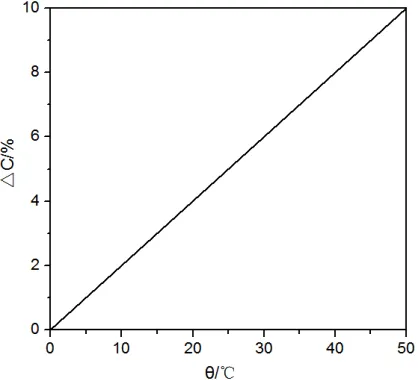
The change of sound speed with increase of temperature is shown in figure 2.

Fig. 2. Increment diagram of sound temperature velocity in air

In the process of the temperature changing from 0 DEG C to 40 DEG C, there will be a change of about 7% of the speed of sound. As a result, in order to improve the accuracy of ultrasonic ranging, when calculating, it needs to consider the influence of temperature, and to revise it. In general, (5) is used to modify the spread velocity in the air.

c

=

331

+

0.6

!

NLOS (non line of sight). If the transmission between mobile anchor nodes and unknown nodes is the transmission of non line of sight, it needs to transmit the infor-mation through the refraction of obstacle and reflection. In this case, the ultrasonic transmission will transmit for a longer time, which will result in that the calculated distance is too large, and the ranging has errors.

Directivity of ultrasonic transmitter and receiver. In general, the ultrasonic sensor emission is not full directional. The strengths of transmit signals in different direc-tions are very different, and the received signal strength is also very different. The signal strength, in general, in ultrasonic wave emitted by the transmitter at 0 degrees offset, is the largest, while in 50 degrees offset, the signal strength will have a signifi-cant decline.

arrival time, thus increasing the ranging distance [8]. In addition, with the increase of transmission distance, the ultrasonic signal has a certain attenuation. Therefore, the larger the transmission distance is, the more serious the ultrasonic attenuation will be. At the receiving end, the more the time spent for amplification of signal. This will cause the time delay, which will make the measured distance larger than the actual distance. This is the error is caused by the ultrasonic receiving.

Software processing delay. Software processing delay refers to the software pro-cessing time after receiving the anchor node signal, which depends on the speed of the processor. And this time will also cause range error so that the measured distance becomes larger.

The frequency and type of ultrasonic sensor. When the ultrasonic spreads in the air, the higher the frequency is, the greater the power will be, and the faster the velocity in the air is. As a result, the attenuation is greater, and the propagation distance is small-er. Consequently, the sensitivity and performance of ultrasonic sensors will affect the ranging accuracy.

Through the above analysis of the ranging error, it is found that in the factors for ranging error, some are random, and some error is due to the system itself. For each node, the error caused by the system is the same, such as the error brought by the temperature, and errors caused by software delay. And in the ultrasonic receiving, because the signal intensity is different, the detection time is not the same, but the detection time will cause the measured distance increases. Assuming that an unknown node receives the information of two different positions of mobile anchor node and calculates the distance to the corresponding position [9]. The subtraction of the two distance is conducted, and we can offset the ranging error caused by the common factors. In this way, their distance difference is closer to the actual distance differ-ence. Thus, the positioning error can be reduced in the positioning operation. We make use of the mathematical form for the description of it in the following.

Generally, it is believed that there is a certain correlation between range errors. Let X and Y be the Gauss white noise with expectation of 0 and the same variance, as well as the same distribution. The relationship coefficient ! between them is:

!

=

E (X

[

!

E(X))(Y

!

E(Y ))

]

E (X

"#

!

E(X))

$%

E (Y

"#

!

E(Y ))

$%

According to (6), we can get:

D

(

X

!

Y

)

=

E

"#

((

X

!

Y

)

!

E

(

X

!

Y

))

$%

=

2(1

!

!

)

D

(

X

)

hyperbola positioning is relatively large, and the process is more complex, which also uses the estimation algorithm. As a result, based on hyperbola positioning, this paper makes improvement. The hyperbola is replaced by asymptote for positioning. Accord-ing to the knowledge learned in high school, a hyperbola will correspond to the two lines. And the definition of asymptote is that if a point on the curve along the curve tends to infinity, the distance from the point to a straight line tends to zero, and then the line is called asymptote for the curve. We can use the asymptote of the hyperbola to replace hyperbola function because the asymptote is the line that hyperbola infi-nitely close to. If we can use asymptote to replace hyperbola, it can bring such bene-fits. Because the asymptote is a straight line, he process of calculation is relatively simple, and it is easier to calculate the the intersection of two lines than the intersec-tion of the two curves. The calculaintersec-tion amount is small, so it can reduce the computa-tional complexity and hardware devices are easy to implement, thus reducing the cost of positioning. The calculation process is simple so that it can save energy, and ener-gy is a very important performance index in the wireless sensor networks.

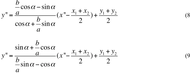
(8) and (9) are the asymptote equations for hyperbola with the distance difference from (x1, y1) and (x2, y2) to two intersections of 2a.

y"

=

b

a

cos

!

!

sin

!

cos

!

+

b

a

sin

!

(x"

!

x

+

x

2

)

+

y

+

y

2

y"

=

sin

!

+

b

a

cos

!

b

a

sin

! !

cos

!

(x"

!

x

+

x

2

)

+

y

+

y

2

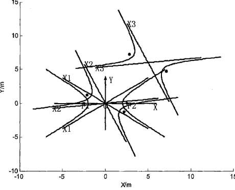
Fig. 3. Hyperbola and Asymptote

By the above algorithm, we can make a general evaluation of the hyperbola and asymptote positioning algorithm, and compared with the algorithm using hyperbola for positioning, the calculation process of asymptote is relatively simple, not related to the problem of solving quadratic equations. In addition, in the solution for intersec-tion, the amount of calculation is greatly reduced. The asymptote is just infinite close of hyperbola, but it is not hyperbola. As a result, the asymptote itself will bring the error, which is the one aspect. In addition, because a hyperbola has two lines, the number of intersection points is not only one. Then, the measured distance infor-mation is applied to test the intersection, to see the distance of which intersection to anchor nodes at different positions is the closest to the measured distance, and then the intersection is taken as the location point. Through the above analysis, there are some benefits for replacing asymptote by hyperbola, but it also brings unfavorable factors. In later chapters, through the simulation, we will prove that the positioning accuracy of positioning through replacing the hyperbola by asymptote has been sig-nificantly improved as compared to the original algorithm. It indicates that the posi-tioning error caused by replacing the hyperbola by asymptote is very small, and the proportion in the position error is relatively small. Moreover, the total amount of computation is no more and complicated than that of the original algorithm.

4

Experimental simulation and result analysis

4.1 Hyperbola and asymptote positioning algorithm implementation process

and all the unknown nodes are equipped with an ultrasonic receiving device. The mobile anchor node moves every certain distance, it sends the ultrasonic signal around; when the anchor node transmits ultrasonic signals around, at the same time, it also transmits radio frequency signal. RF (Radio Frequency) signal contains infor-mation: the coordinate information of anchor nodes. When the nodes to be positioned receive radio frequency signals sent by the mobile anchor node, the time is record as T1, and then open ultrasonic receiver to wait for the arrival of the ultrasonic wave. When the ultrasonic wave arrives, the time is recorded as T2. Because the radio signal propagation speed is far greater than that of the ultrasonic, radio propagation time is ignored and then the coordinate information and the ultrasonic propagation time are correspondingly stored.

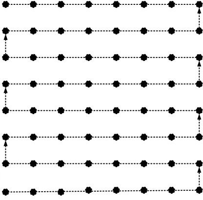
The move locus of single track method designed is shown in Figure 4. The design environment is in a regular rectangular area, the mobile anchor node moves along the trajectory as shown in Figure 4. When reach a particular point, it emitted radio fre-quency signal and ultrasonic signal. And the nodes in the communication radius scope receive the the signal, and through its own calculation, the distance to the specific location of the mobile anchor node can be obtained. After receiving the distance to different position of more than three mobile anchor nodes, we can locate the unknown nodes. Therefore, the three position of the mobile anchor node can be used to calcu-late the two hyperbolas. Because a hyperbola has two asymptote, the intersection obtained is four. It also needs to determine which is the approximate coordinates of unknown nodes, and thus it needs to use prior knowledge to judge. The measures taken in the paper is to take the distance measured in the previous part as the basis of judgment. We can compare the distance between the four nodes to the anchor node and the measured distance, and find the closest point as the coordinates of the un-known node.

According to the above conditions, simulation is carried out. The selected area is 600 * 600 square meters area, general nodes are randomly deployed in the area, and the number of deployed is 50. The premise of the simulation experiment design is based on the assumption that the ranging error obeys normal distribution (0, 1). Set the anchor node communication radius to 1.5 times of each anchor node moving dis-tance. With the change of the distance of each movement, its communication radius increase proportionally. According to the above conditions, simulation is carried out, and 100 times repeated experiments are done and simulation results are obtained.

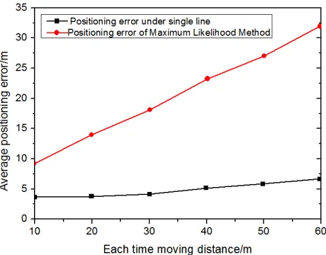
Through simulation, it can be found that most nodes can get their own approximate position, and the point at the boundary can basically achieve the positioning, but there are individual nodes, because of the too great error, will cause the positioning failure. In the above environment, the simulations of the algorithm positioning and maximum likelihood method positioning are performed, respectively. They are compared, and the simulation results are shown in figure 5.

Fig. 5. Average error in the condition of moving distance difference every time

4.2 Comparison with the increase of ranging error

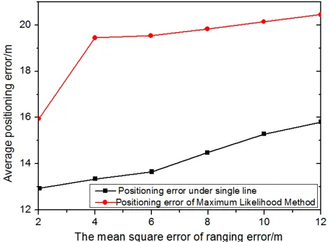
The simulation environment still chooses 600 * 600 square meters area, general nodes are randomly deployed in the general area, and the number of deployed is 50. The simulation results are obtained by the 100 times repeated experiments. The simu-lations of the positioning algorithm and the maximum likelihood method are per-formed, respectively, in the above location environment. They are compared, and the simulation results are shown in figure 6.

Fig. 6. Average error in the condition of increasing distance error

It can be seen from the figure that, the error of hyperbola asymptote positioning al-gorithm is less than that of the maximum likelihood method. From a single aspect, with the increase of the ranging error, the positioning accuracy is also gradually in-creasing. In terms of the hyperbola asymptote positioning method, with the increase of measurement error, the positioning error also increase, and the growth rate will increase with the increase of ranging error. The ranging error increases the same pro-portion, the positioning error may cause a greater proportion increase. In conse-quence, it is necessary to control the increase of ranging error as far as possible, to ensure the change of positioning precision. The ranging error is affected by environ-ment, temperature, humidity, and some sudden changes. Therefore, when positioning, we should make specific analysis of the positioning error based on the specific envi-ronment, so as to make it reasonably use the nature of ranging.

5

Conclusions

distance measurement technology is further explored. The hyperbolic positioning algorithm is improved, and asymptote positioning algorithm is proposed. The simula-tion results show that the posisimula-tioning accuracy of hyperbolic asymptote is higher than that of the maximum likelihood method in computational complexity. The hyperbolic asymptote to judge the intersection is a step more than the maximum likelihood meth-od. But the maximum likelihood method requires the quadratic equations calculation. Therefore, in terms of the computation, the two are almost in the same level, and the hyperbola asymptote positioning has certain advantages.

6

References

[1]Hao, X. (2016). Wireless sensor networks positioning based on graph embedding with polynomial mapping: Computer Networks, 106: 151-160. 2 https://doi.org/10.1016/j.com net.2016.06.032

[2]Chakchai S. (2016). Soft computing-based positionings in wireless sensor networks: Per-vasive and Mobile Computing, 29: 17-37. https://doi.org/10.1016/j.pmcj.2015.06.010 [3]Diego, V. Q. (2017). Survey and systematic mapping of industrial Wireless Sensor

Net-works: Journal of Network and Computer Applications, 97: 96-125. https://doi.org/10.1016/j.jnca.2017.08.019

[4]Tashnim, J. S. (2016). Advances on positioning techniques for wireless sensor networks: A survey: Computer Networks, 110: 284-305. https://doi.org/10.1016/j.comnet.2016.10.006 [5]Colin, E. (2017). positioning in wireless sensor networks: A Dempster-Shafer evidence

theoretical approach: Ad Hoc Networks, 54: 30-41. https://doi.org/10.1016/j.adhoc. 2016.09.020

[6]Eliyeh, M. (2017). A robust method for underwater wireless sensor joint positioning and synchronization: Ocean Engineering, 137: 276-286. https://doi.org/10.1016/j.oceaneng. 2017.04.006

[7]Angel, S. (2016). Cooperative method for wireless sensor network positioning: Ad Hoc Networks, 2016: 61-72. https://doi.org/10.1016/j.adhoc.2016.01.003

[8]Slavisa, T. (2017). Distributed algorithm for target positioning in wireless sensor networks using RSS and AoA measurements: Pervasive and Mobile Computing, 37: 63-77. https://doi.org/10.1016/j.pmcj.2016.09.013

[9]Alessandro, R. (2013). An integrated system based on wireless sensor networks for patient monitoring, positioning and tracking: Ad Hoc Networks, 11(1): 39-53. https://doi.org/10.1016/j.adhoc.2012.04.006

[10]Guangjie, H. (2013). positioning algorithms of Wireless Sensor Networks: a survey: Tele-communication Systems, 52(4): 2419-2436. https://doi.org/10.1007/s11235-011-9564-7

7

Authors

WuBaolin Su, Quanyu Zhang and Boyang Zhang are with College of Electri-cal Engineering, Suihua University, Heilongjiang, China.