Algorithms and Performance Analysis for Synchrophasor and Grid State Estimation

(1)

PhD Dissertation

International Doctorate School in Information and Communication Technologies

DISI - University of Trento

ALGORITHMS AND PERFORMANCE ANALYSIS FOR

SYNCHROPHASOR AND GRID STATE ESTIMATION

Grazia Barchi

Advisor:

Prof. Dario Petri

University of Trento

(2)

(3)

(4)

(5)

Abstract

The electrical quantities of future power networks are expected to exhibit strong fluc-tuations caused by dynamic bidirectional energy flows transferred from/to a multitude of “prosumers”. Such variations have to be accurately measured in real-time either for efficient power distribution or for safety and protection purposes. This task can be ac-complished by the Phasor Measurement Units (PMUs), which measure the phasor of voltage or current waveforms synchronized to the Coordinated Universal Time (UTC). Accuracy of synchrophasor measurements is one of the many open challenges that need to be addressed in order to guarantee smart grid reliability and availability. Synchrophasor measurement has gained an undisputed relevance in the research community working on power delivery issues for various reasons. Among them, state estimation (SE) of both transmission and distribution networks is one of the most important. Within this general context, this dissertation covers two complementary topics.

In the first part, starting from the concept of synchrophasor and from the definition of the parameters to evaluate PMU performances, useful guidelines to design a filter-based synchrophasor estimator are provided. Afterwards, an extensive performance comparison of some state-of-the-art synchrophasor estimation algorithms is reported in most of the static and dynamic conditions described in the IEEE Standards C37.118.1-2011. Also, a novel technique able to address both static and dynamic disturbances is presented and analyzed in depth. In this respect, special attention is devoted to phasor angle estimation accuracy, which is particularly important for active distribution networks.

The second part of the dissertation is focused on the role and the impact of PMUs for grid state estimation. After recalling the state estimation problem and the traditional Weighted Least Square (WLS) technique to solve it, a general uncertainty sensitivity analysis to different types of measurements is introduced and justified both theoretically and through simulations. Afterwards, the effect of a growing number of PMUs on WLS-based state estimation uncertainty is evaluated as a function of instrumental accuracy and line parameters tolerance. Finally, a Bayesian linear state estimator (BLSE) based on a linear approximation of power flow equations for distribution networks is presented. The main advantage of BLSE is that in most cases it is so accurate as the WLS technique, but it is computationally lighter, faster and more stable from the numerical point of view.

(6)

(7)

Acknowledgements

This work is the conclusion of three years of passionate research, which has involved also several other people.

First of all, I would like to express my gratitude to my advisor, Prof. Dario Petri, for his guidance and motivation during the whole PhD program. I would like to thank Dr. David Macii and Dr. Daniele Fontanelli for their suggestions and precious support.

Special thanks goes to Prof. Kameshwar Poolla and to Prof. Alexandra von Meier for the opportunity that they gave me to be a visiting scholar at the University of California, Berkeley; and to Prof. Luca Schenato, Dr. Reza Arghandeh and Dr. Guido Cavraro for the fruitful scientific collaboration while I was there.

Finally, I would like to thank my family and my friends for their endless support and the colleagues who I have met in these years.

(8)

(9)

Publications as author and co-author

International Journals

[J.1 ] G. Barchi, D. Fontanelli, D. Macii and D. Petri, “On the Accuracy of Phasor Angle Measurements in Power Networks”, on IEEE Trans. Instrumentation and Measurement,vol., no., pp., . 2015

[J.2 ] G. Barchi, D. Macii, D. Belega and D. Petri, “Performance of synchrophasor estimators in transient conditions: A comparative analysis”, IEEE Trans. Instru-mentation and Measurement,vol.62, no.9, pp.2410-2418, Sept. 2013

[J.3 ]G. Barchi, D. Macii and D. Petri, “Synchrophasor Estimators Accuracy: A Com-parative Analysis,” IEEE Trans. Instrumentation and Measurement,vol.62, no.5, pp.963-973, May 2013

International Conference Proceedings

[I.1 ] L. Schenato, G. Barchi, D. Macii, R. Arghandeh, K. Poolla and A. Von Meier, “Bayesian Linear State Estimation using Smart Meters and PMUs Measurements in Distribution Grids,”IEEE International Conference on Smart Grid Communica-tions 2014, pp. 1-6, Venice, Italy, 3-6 Nov 2014.

[I.2 ] D. Macii, G. Barchiand D. Petri,“Uncertainty Sensitivity Analysis of WLS-based Grid State Estimators,”IEEE International Workshop on Applied Measurements for Power Systems, pp. 1-6, Aachen, Germany, 24-27 Sep 2014.

[I.3 ]D. Macii,G. Barchi and L.Schenato, “On the Role of Phasor Measurement Units for Distribution System State Estimation,” IEEE Workshop on Environmental, Energy and Structural Monitoring, pp. 1-6, Naples, Italy, 17-18 Sep 2014.

[I.4 ]G. Barchi, D. Fontanelli, D. Macii and D. Petri, “Frequency-domain Phase Mea-surement Algorithms for Distribution Systems,” IEEE International Instrumenta-tion and Measurement Technology Conference (I2MTC), pp. 1828-1833, Montev-ideo, Uruguay, 12-15 May 2014.

[I.5 ]G. Barchi, D. Macii, and D. Petri, “Phasor Measurement Units for Smart Grids: Estimation Algorithms and Performance Issues”, AEIT Meeting 2013, Oct. 2013.

(10)

[I.7 ]G. Barchi, D. Macii and D. Petri,“Effect of transient conditions on DFT-based synchrophasor estimator performance”, IEEE International Workshop on Applied Measurements for Power Systems (AMPS), pp. 1-6, Sep. 2012.

[I.8 ] G. Barchi and D. Petri,“An improved dynamic synchrophasor estimator”, IEEE International Energy Conference and Exhibition (ENERGYCON), pp. 812-817, Sep. 2012.

[I.9 ]G. Barchi, D. Macii and D. Petri, “Accuracy of One-cycle DFT-based Synchropha-sor Estimators in Steady-state and Dynamic Conditions”, IEEE International In-strumentation and Measurement Technology Conference (I2MTC), pp. 1529-1534, May 2012.

(11)

(12)

Chapter 1

Introduction

1.1

Context of the research

(17)

2 Introduction

Figure 1.1: Total carbon dioxide emissions from the consumption of energy (millions metric tons) [Source: Energy Information Administration, U.S. Government]

flows supported by suitable infrastructures for both communication and protection. The introduction of information and communication technologies (ICT) in the power networks creates the so-called smart power grids. In the near future the smart grid will allow us to integrate small production plants and new loads devices (e.g. the electric vehicles) thus giving to prosumers (producers-consumers) an active role in electricity pricing. At the same time continuous service, adequate amplitude and frequency stability at the minimum cost, security, and an acceptable impact on the environment will have to be ensured and possibly improved. The term continuous service refers mainly to reliability and availability of the network [3]. Indeed, in the recent years much research work has focused on solutions to increase transmission capacity with a low environmental impact, to improve system operation after the integration of variable energy resources (VERs) such as wind-based or photovoltaic plants [4], and to avoid catastrophic black-outs like those happened in the North-East of U.S. and in Italy in 2003.

(18)

Context of the research 3

Figure 1.2: Total primary energy consumption per capita (millions Btu per person) [Source: Energy Information Administration, U.S. Government]

(19)

4 Introduction

Figure 1.3: Total renewable electricity net generation (Billions kWh) [Source: Energy Information Ad-ministration, U.S. Government]

the role of this type of instruments. These applications include (but are not limited to) fast protection equipment (i.e. with response times in the order of few ms) [8], voltage stability and oscillation monitoring [9, 10], fault detection and location [11], islanding maneuvers [12, 13], state estimation [14] and load modeling [15].

1.2

Objectives and contribution of the research work

Next-generation PMUs are required to exhibit superior accuracy and responsiveness at lower costs. Also, they are supposed to measure not only phasors, but also waveform frequencies and frequency changes. Even if PMU performances are affected by different uncertainty sources, the estimation algorithm plays an essential role in instrument per-formance. Several novel estimation techniques have been developed in the last years in the attempt of both mitigating the effect of static disturbances (such as harmonics and inter-harmonics) and tracking fast phasor changes due to intrinsic variations of the net-work operating conditions. Due to the recent definition of various algorithms based on the so-called phasor dynamic model, a detailed comparison between their performances can be hardly found in the literature. So one of the primary goals of this research work is to fill at least partially this gap by presenting and testing quite famous estimation algorithms in a common and widely accepted framework: the conditions described in the IEEE Standards C37.118.1-2011 and its Amendment IEEE C37.118.1a-2014.

(20)

Objectives and contribution of the research work 5

be devoted to the problem of phasor angle estimation, which is quite unexplored and is particularly important at the distribution level, where PMU deployment is expected to be massive in the near future.

The second part of the thesis covers a complementary aspect, namely the role of PMUs for grid state estimation, which is considered as one of the most relevant applications of synchrophasor measurements. Many works related to this topic already exist, but most of them focus on optimal PMU placement to maximize state estimation accuracy or to minimize the overall monitoring costs. In this thesis instead the emphasis is mainly on how the number and the accuracy of synchrophasor measurements influence state estimation especially at the distribution level. At first, a theoretical analysis of the sensitivity to measurement uncertainty of the well-known Weighted Least Squares (WLS) estimation technique is reported (properly supported by meaningful simulations) in order to identify what types of measurements are most critical for state estimation. Thus this analysis paves the way to a deeper understanding of the impact of PMUs on state estimation uncertainty in distribution systems. Then, a novel linear Bayesian state estimation algorithm relying on both PMU-based phasor measurements and real/reactive power pseudo-measurements is proposed in order to achieve reasonably accurate state estimates with less numerical problems and with a lower computation burden than using the WLS approach.

In conclusion, the thesis is structured as follows.

Chapter 2 deals with an overview of synchrophasor measurements and PMUs. At first, the common structure of PMUs is described, along with how the synchrophasor data are collected. Then, important definitions as well as some static and dynamic testing conditions based on the IEEE Standard C37.118.1-2011 are introduced. Such testing conditions will be also used in Chapter 3 and Chapter 4. Finally, some general guidelines to design a filter for synchrophasor estimation are reported.

In Chapter 3 three state-of-the-art techniques for synchrophasor estimation are de-scribed and their performances are extensively analyzed and compared under the steady-state and dynamic conditions reported in the IEEE Standard C37.118.1-2011.

In Chapter 4 a novel synchrophasor estimator is proposed and validated through simu-lations in most of the conditions reported in the Standard. In view of using this algorithm in PMUs for distribution systems (where a superior phase measurement accuracy is re-quired), the phasor angle measurement accuracy alone is analyzed and compared with the accuracy of other two state-of-the-art algorithms.

(21)

6 Introduction

(22)

Chapter 2

Synchrophasors and PMUs

As stated in Chapter 1, the PMUs are the key elements of the WAMS, as they measure the phasors of different waveforms over a wide area at the same time. This chapter presents at first an overview of a common PMU architecture which the specific function of each block. Then, the main concepts taken from the current synchrophasor Standard IEEE C37.118.1-2011 and used in the rest of the thesis are introduced. At last some guidelines to design suitable filters for synchrophasor measurement are proposed.

2.1

Phasor Measurement Unit

The first prototypes of PMUs were built at the Virginia Tech in the early 1980s. At present, PMUs by different manufacturers may differ in various important aspects. Nonethe-less, a quite general PMU architecture is shown in Fig. 2.1 [6]. The input waveform, i.e.

Anti-aliasing filter

A/D Converter

Phasor Micro-processor Phase-locked

oscillator GPS

receiver Modem

Analog inputs

Figure 2.1: A common Phasor Measurement Unit architecture. Source: [6].

Part of this chapter was published in

(23)

8 Synchrophasors and PMUs

voltage or current, is acquired by a signal conditioning module (that typically just con-sists of an anti-aliasing filter), followed by an Analog-to-Digital Converter (ADC). The sampling clock signal (with a frequency in the order of tens of kilo-samples/second) is phase-locked with a train of pulses synchronized to the UTC through a GPS receiver or through wired synchronization protocols such as IRIG-B or the Precision Time Protocol (PTP) [16]). The digitized electrical waveform is sent to an embedded processing com-ponent, such as a microprocessor (µP), which calculates the synchronized phasor using a specific estimation algorithm, frequency and rate of change of frequency (ROCOF). Addi-tionally, it relies on the synchronization block to time-stamp the measurements. Finally, the estimated values are transmitted to other PMUs or the Phasor Data Concentrators (PDCs), which are able to collect data from different PMUs and align their in time. Gen-erally, four types of files are exchanged between PMUs, i.e. configuration, header and data files. In addition, command files are used to control the PMUs from a higher level of the network hierarchy [17]. The PMUs are placed and installed in power system substa-tions. In order to use PMUs measurement in different applications (e.g. state estimation, fault detection, stability estimation, control...), they have to be controlled remotely. For such reasons a hierarchical architecture that involves PMUs, communication systems and PDC, as shown in Fig. 2.2 has to be realized. The PMUs measurement data can be stored locally for diagnostic purposes or can be sent to PDCs for high-level filtering and mon-itoring. Many applications require data from several PMUs. After bad data exclusion, time-stamps alignment, coherent records are gathered by the PDCs themselves. In order to extend the PDCs data-gathering capability the Super Data Concentrator or direct ( monitoring system/station) is used at a higher hierarchical level.

PMU

Phasor Data Concentrator

Super Data Concentrator

PMU PMU PMU

Phasor Data Concentrator

Storage Storage

Data storage Real-time

application

(24)

Concept of synchrophasor in the series of standards

IEEE C37.118-2011 9

2.2

Concept of synchrophasor in the series of standards

IEEE C37.118-2011

The goal of PMU is to perform real-time and accurate measurements of the phasors synchronized to the UTC, in order to track possible variations, to detect abnormal phe-nomena and to support control operations in power grid. However, to operate correctly it is necessary that synchrophasor measurements and data messaging are compliant with the definition and the performance requirements of suitable Standards. The synchrophasor definition was standardized for the first time in 1995 in the IEEE Std 1344. This standard introduces also concepts such time accuracy, synchronization to UTC and requirements for waveform sampling. Ten years later, more complete and meaningful changes were in-troduced in the IEEE Std C37.118-2005. This specifies how to evaluate the measurement performance and the message structure for synchrophasor data. It defines the Total Vec-tor Error (TVE) as the main accuracy index and its limits in steady-state conditions in order to fulfill the compliance requirements. However the need to analyze synchrophasor performance also under dynamic conditions (i.e in presence of amplitude/phase variations or frequency ramp) led to the current and revised version in late 2011.

The new standard, IEEE Std C37.118-2011, is divided in two parts: the first one, i.e IEEE Std C37.118.1-2011 in the following simply called ”the Standard” [18], provides the definitions of synchrophasor, waveform frequency and rate of change of frequency (ROCOF). Moreover it deals with the compliance boundaries and tests to evaluate the performance of PMUs under steady-state and dynamic conditions. The second part, IEEE Std C37.118.2-2011 deals with the synchrophasor data transfer and data formats [17]. Two performance classes are defined in the Standard IEEE C37.118.1-2011, i.e. P-class andM-class, in order to meet orthogonal applicative needs. TheP-class PMUs are mainly oriented to those applications requiring a fast measurement response time (e.g. for safety-critical, protection purposes). Conversely, the M-class PMUs are used when measurement accuracy is more important than measurement speed. All the compliance tests under steady-state and dynamic conditions are specified in the Standard. Recently, an amendment of the Standard, called IEEE C37.118.1a-2014 was published in order to fix some inconsistencies and to relax some constraints difficult to meet especially re-lated to frequency and ROCOF estimation (see 2.2.1). In spite of the recent publication of Amendment IEEE Std C37.118.1a-2014 in the rest of the dissertation the IEEE Std C37.118.1-2011 will be considered as reference document, except in the few particular cases.

(25)

Frames per second, for 50 Hz and 60 Hz systems are listed in the Tab.2.1. Other reporting rates(100 frames/s or 120 frames/s or rates lower than 10 frames/s, such as 1 frames/s), are also encouraged.

Table 2.1: PMU reporting rates[18].

System frequency 50Hz 60 Hz

Reporting rates (Fs - frames per second) 10 25 50 10 12 15 20 30 60

In the following the main concepts introduced in the Standard and used in the rest of dissertation are presented and explained.

2.2.1 Synchrophasor, frequency and ROCOF definitions Model signal and synchrophasor

In AC power systems an electrical waveform (i.e. current or voltage) x(t) of nominal frequency f0 (i.e. 50 Hz or 60 Hz) can be expressed as

x(t) =Acos(2πf0t+φ) (2.1)

where A is the amplitude and φ is the initial phase. A common representation of (2.1) through its complex static phasor is defined as

¯

X = √A

2e jφ

. (2.2)

A synchronized phasor or synchrophasor of an electrical signal in (2.1) is the value ¯X in (2.2) at a known reference time, tr, synchronized to the Coordinated Universal Time (UTC) [18]. The convention reported in the Standard for synchrophasor representation is shown in Fig. 2.3. On the left, the synchrophasor angle is 0 degrees when the maximum of (2.1) occurs at the UTC second rollover, on the right the synchrophasor angle is –90 degrees when the positive zero crossing occurs at the UTC second rollover.

In steady-state conditions the waveform frequency, amplitude and phase parameters can be considered as constant during the whole observation interval, while in a more realistic scenario they are affected by both amplitude and phase variations caused by power oscillations and other disturbances. So, in order to analyze the behavior of a power system under both steady-state and dynamic conditions, a generalization of the electrical waveform model in (2.1) is

(26)

Concept of synchrophasor in the series of standards

IEEE C37.118-2011 11

t=0 (1 PPS)

𝑋 = 𝐴₂

A _A

t=0 (1 PPS)

𝑋 = 𝐴₂𝑒−𝑗𝜋2

Figure 2.3: Convention for synchrophasor representation [18].

whereA,f0andφhave the same meaning as in (2.1), 2πδf0tis the accumulated phase shift due to the static fractional off-nominal frequency offsetδ,εa(t) describes the time-varying amplitude fluctuations, εp(t) includes possible phase fluctuations and η(t) generally in-cludes possible narrowband components (e.g. harmonics and additive wideband noise).

Since both amplitude and phase in (2.3) change as a function of time, the synchropha-sor at the UTC reference time tr is defined as

¯

Xr = ¯X(tr) = A(tr)

√

2 e

jϕ(tr) ₌ _√A

2[1 +εa(tr)]·e

j[2πf0(1+δ)tr+εp(tr)+φ] _(2.4)

Frequency and rate of change of frequency estimation

A last generation PMU is able to measure not only the synchrophasor, but also the waveform frequency and the rate of change frequency estimation (ROCOF). Starting from equation (2.3), ifεa(·) and η(·) are negligible, the sinusoidal signal can be rewritten as

x(t) =Acos[ϕ(t)] (2.5)

whereϕ(t) = 2πf0(1 +δ)t+εp(t) +φ. Thus frequency of signal x(t) in (2.5) at timetr is defined by

fr =f(tr) = 1 2π

dϕ(tr)

dt =f0+f0δ+

1 2π

dεp(tr)

dt =f0+ ∆f(tr) (2.6) where ∆f(tr) is the instantaneous deviation frequency from the nominal value. Finally, the corresponding ROCOF is defined as follow

ROCOFr =ROCOF(tr) =

df(tr)

dt =

1 2π

d2_ϕ(t r)

dt2 =

d∆f(tr)

(27)

Figure 2.4: Graphical representation of TVE definition.

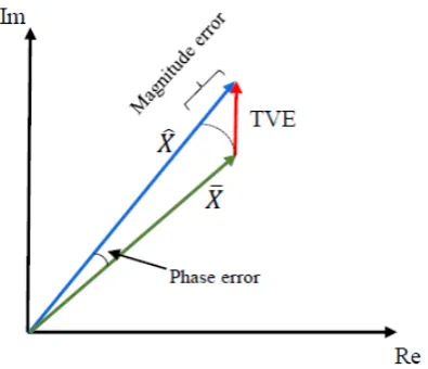
2.2.2 Measurement evaluation Total Vector Error

The estimation accuracy of the synchrophasor measured by PMU is in the Standard typically expressed in terms of Total Vector Error (TVE). Indeed, TVE combines the effect of magnitude errors, phase errors and synchronization uncertainty. If we denote the estimated phasor as ˆX¯ and the actual phasor value as ¯X, the TVE can be defined as

T V Er =

|Xˆ¯r−X¯r|

|X¯r|

(2.8)

where the subscriptr indicates that both the estimated and the actual value of the phasor are computed at the reference time tr.

Frequency and ROCOF measurement error

In the last version of the Standard the frequency measurement error and the ROCOF measurement error are given by the difference between the actual values and the estimated values. They are defined as

F Er = |fr−fˆr|=|∆fr−∆ ˆfr| (2.9)

RF Er =

dfr

dt −

dfˆr dt

(2.10)

(28)

Reference signal processing models 13

T

V

E

[%

]

Time Step input

t=0

response time 1%

Figure 2.5: Example of amplitude step change over the time [18].

Response time and delay time

In order to evaluate the performance of an algorithm when sudden amplitude or phase change occurs, the Standard suggests to evaluate both the response time and the delay time. Especially the response time will be used in the following. However both definitions as they are reported in the Standard are recalled.

The measurement response time “is the time to transition between two steady-state mea-surements before and after a step change is applied to the input. It shall be determined as the difference between the time that the measurement leaves a specified accuracy limit and the time it reenters and stays within that limit when a step change is applied to the PMU input.[...] Accuracy limits are the TVE, FE, and RFE values for the phasor, frequency, and ROCOF measurements, respectively”[18]. In the case of TVE (that is the only pa-rameter considered in next sections) the limit specified by the Standard is set equal to 1%. In Fig. 2.5 an example of TVE response time resulting from an amplitude step is shown.

The delay time is defined as “the time when the stepped parameter achieves a value that is halfway between the starting and ending steady-state values”[18].

2.3

Reference signal processing models

(29)

Antialiasing

filter ADC

Analog front-end

LP filter W(ω)

Synchronized

Clock to UTC oscillator (Quadrature f0) sin 2πf0 cos2πf0

Re

Im

x(t) x[n]

Mag

Ang

Figure 2.6: Block diagram of the synchrophasor estimation model suggested in the Standard IEEE C37.118.1-2011.

down-conversion and digital low-pass filtering of the in-phase and quadrature components of voltage and current waveforms. Two examples of low-pass filters having quite different performances in terms of latency and accuracy are also reported in the same annex: one for protection-oriented applications (P-class reference model) and the other when high measurement accuracy is required (M-class reference model). Starting from (2.3), if the phase fluctuations εp(t) are negligible, but δ6= 0, then phasor (2.4) rotates at a constant rate δf0. The block diagram of the basic synchrophasor estimation model described in Annex C of the Standard is shown in Fig. 2.6 [18]. The expression of the estimator is

ˆ ¯

Xr =

 



√

2 W(0) ·

PN2−1 n=−N−1

2

w[n]x[r+n]·e−jM2π(r+n) N odd

√

2 W(0) ·

PN2

n=−N₂ w[n]x[r+n]·e

−j2_Mπ(r+n) _N _even (2.11)

where:

• x[·] is the digitized input waveform sampled at a ratefs by the front-end analog-to-digital converter (ADC);

• N is the number of impulse response coefficients of the chosen filter;

• M = fs/f0 represents the number of samples in one nominal waveform cycle. Ac-cordingly, 2π/M is the angular frequency of the two quadrature digital sine-waves that are mixed with the input signal;

• w[·] is the impulse response of the adopted low-pass Finite Impulse Response filter;

• W(ν) is the frequency response of the filter, ν = f /fs is the normalized digital frequency and W(0) is the filter DC gain.

(30)

Reference signal processing models 15

is odd, whereas it lies between two subsequent samples (i.e., at time (r−1/2)/fs), when N is even. As a consequence, while W(ν) is generally designed to provide a linear phase response, in (2.11) no phase delay is introduced by the filter (i.e. its phase response is zero). Notice that if we refer to C = N/M as the number of nominal waveform cycles inN samples, (2.11) can be equivalently regarded as the C−th sample of the windowed Discrete-time Fourier Transform of the sequence x[·] centered at time tr. Therefore, the estimation approach described in [18] and the windowed DFT-based phasor estimators basically coincide, since the adopted sliding window simply acts as a filter [19].

2.3.1 P-Class filter model

The Annex C suggests a fixed-length two-cycle triangular FIR filter, with an odd number of samples, regardless of PMU reporting rates. The filter coefficientsw[n] are:

w[n] =

1− 2

N + 2|n|

(2.12)

where n = −N/2, .., N/2 and N is the filter order. The P-class filter works well at the nominal frequency when the observation interval matches exactly the period of the collected sine-wave. However in presence of off-nominal frequency deviations, a magnitude correction applied to the final phasor is required [18].

2.3.2 M-Class filter model for phasor

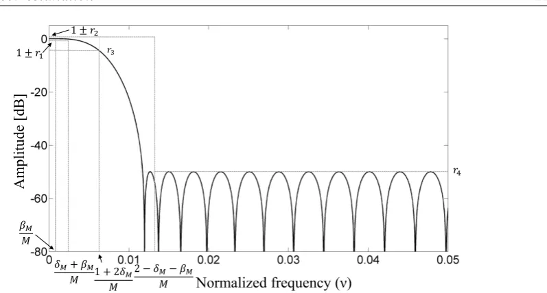
TheM-class requires that the filter is able to attenuate significantly the signals above the Nyquist frequency for a given reporting rate. This filter provides more accurate results in the presence of noise and interfering signals, but with longer reporting delays. In the amendment to the Standard the filter mask specifications are shown in Fig. 2.7. The window coefficients can be computed with

w[n] =

sin2π× 2Ff r

Fsamp ×n

2π× 2Ff r

Fsamp ×n

h[n] (2.13)

(31)

Figure 2.7: Reference algorithm filter frequency response mask specification for M class [18].

2.4

Proposed guidelines for filter-based

synchrophasor estimation

As shown in paragraph 2.3.1 and 2.3.2, the Standard reports two examples of low-pass filters with different performances in terms of latency and accuracy. However, no clear filter design criteria are provided. In [20] and [21] the authors describe and analyze the performance of two orthogonal filters with time-frequency characteristics that are particularly suitable for fault location and measurement. In [22] a raised-cosine filter with a negligible phase distortion is described to halve the phasor estimation delay. In [23] and [24] two filters for P-class and M-class phasor estimation, respectively, are proposed to improve the performance of the basic model reported in Annex C of the Standard.

In this section, the same model is used as a starting point to identify optimal filter design criteria. Some simulation results support the proposed analysis.

2.4.1 Filter design criteria

According to (2.3), an electrical waveform in dynamic conditions can be regarded as an amplitude and phase modulated signal around a carrier of frequency (1 +δ)·f0. If we suppose, for the sake of simplicity, that the modulating signals are two sine waves, εa(t) and εp(t) can be expressed as

(32)

Proposed guidelines for filter-based

synchrophasor estimation 17

and

εp(t) = kpcos[2πδpf0t+αp] (2.15) where ka (with ka ≤ kaM ) is the amplitude modulation index, δa = fa/f0 is the

corre-sponding fractional frequency,kp (withkp ≤kpM) is the amplitude (expressed in radians)

of the phase modulation signal and δp = fp/f0 is the fractional modulation frequency. Under this assumption, it can be easily proved that the spectrum of (2.3) consists of an infinite series of monochromatic terms located at frequencies [h·(1+δ)+m·δp+l·δa]·f0, for h≤1, andl = –1,0,1 [25]. This is due to the fact each tone resulting from phase modu-lation is in turn modulated also in amplitude, thus generating three spectral components at frequencies (m·δp+l·δa)·f0. The two side terms (i.e., shifted by±δa·f0 with respect to m·δp·f0) are proportional to ka. Moreover, the amplitude of each triple of spectral com-ponents is proportional toJm(kp), i.e. the first-kind Bessel function of order m computed at kp. Since the values of |Jm(kp)|, for a given kp, decrease monotonically as a function of |m|, the effective bandwidth of (2.3) containing 98% of the signal power around the carrier is 2·β ·f0, with β = (kp + 1)δp +δa [25]. Notice that, in accordance with (2.4), εa(t) and εp(t) are intrinsically part of the phasor to be estimated, whereas harmonics in (2.3) represent a disturbance and, consequently, must be suitably filtered to improve synchrophasor estimation. By mixing the digitized input sequence with two quadrature sine-waves of nominal frequency f0 (or equivalently, of normalized frequency 1/M), the fundamental component as well as the modulating terms of (2.3) are down-converted to the baseband, around frequency δ·f0. Thus, if the static fractional frequency offset δ lies in the interval [–δM, δM] (where δM represents the maximum value of the frequency measurement uncertainty assured by the considered PMU), the one-sided normalized filter bandwidth that must be used to preserve both static and dynamic phasor contributions is:

BWp =

(δp+βM)·f0 fs

= δM + (kpM + 1)·δpM +δaM

M , (2.16)

whereβM,δaM and δpM denote the maximum allowed values ofβ, δa and δp, respectively.

Such values can be hardly known a priori. However, for filter design purposes, they can be set in compliance with the requirements of some standard document such as the IEEE C37.118.1-2011 and the amendment IEEE C37.118.1a-2014. It is worth noticing that βM/M is the bandwidth increment needed to track fast phasor fluctuations.

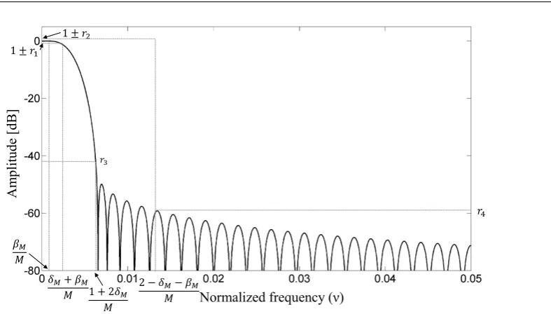
Fig. 2.8 provides a qualitative overview of the main features of the low-pass filter to be used for phasor estimation after signal down-conversion. Parameters r1 and r2 represent the maximum ripple amplitudes in the filter pass-band. In general, the flatness in-band requirements can be relaxed in the frequency interval [±δM/M,±(δM +βM)/M] (i.e.

r2 > r1), because phase and amplitude fluctuations are expected to be quite small (e.g.,

(33)

1

M

1 − 2δ𝑀

M

1 + 2δ_𝑀

M

δ_𝑀

M

𝛽𝑀

M

2

M

1 + 3δ_𝑀

M

1 − 3δ_𝑀

M

2+δ_𝑀

M 1 + 𝑟1

1 − 𝑟1 1 + 𝑟2

1 − 𝑟2

2 +δ_𝑀 + 𝛽_𝑀

M

Static and dynamic band

Image frequency and 3rd_harmonic

2nd_harmonic 2−δ𝑀

M

2 −δ_𝑀 − 𝛽_𝑀

M

𝑟3 𝑟4

Figure 2.8: Qualitative representation of the filter design requirements in the frequency domain, including static and dynamic in-band flatness specifications, second-order and third-order harmonic attenuation and image tone cancellation.

the transition band of the filter must not exceed (1–2δM)/M. This value corresponds to the lower end of the frequency interval [(1–2δM)/M,(1+2δM)/M], where the second-order signal harmonic lies as a result of signal down-conversion.

(34)

i.e.

T V E =

ˆ ¯ Xr−X¯r

X¯r

= ˆ ¯

Xb,r+ ˆX¯i,r+

PH

h=2Xˆ¯h,r−X¯r

X¯r

6 ˆ ¯

Xb,r−X¯r

X¯r

+ ˆ ¯ Xi,r X¯r

+ H X h=2 ˆ ¯ Xh,r X¯r

, (2.17)

where ˆX¯b,r is the baseband waveform component of the estimated phasor (namely the component of interest of the input signal), ˆX¯i,r is the error contribution caused by the infiltration of the image component and ˆX¯h,r, for h= 1,· · · , H are the error terms due to imperfect harmonics filtering. If the phase modulation index is small enough (namely if kp 1, as it is typically expected in practice), thenJ0(kp)≈1,|J−1(kp)|=|J1(kp)|<0.1 and |Jm(kp)| ≈ 0, for m >1. Therefore, after a few algebraic steps it can be shown that the following inequality holds, i.e.

|Xˆ¯b,r−X¯r |

|X¯r |

< r1+|r2−r1 | ·

h_k aM

2 + k_aM+1

10

i

(1−kaM)

. (2.18)

As far as the image and harmonic contributions are concerned, it is straightforward to show that ˆ ¯ Xi,r X¯_r

+ H X h=2 ˆ ¯ Xh,r X¯_r

X¯_r

6r₄+

r3X2+PH_h₌₃r4Xh X(1−kaM)

. (2.19)

If T V Emax represents the maximum tolerable TVE value, the following general design

conditions must be fulfilled:

• 1−r1 ≤ |W(ν)| ≤1 +r1 with r1 ≤F1·T V Emax forν ∈

0,δM

M

;

• 1−r2 ≤ |W(ν)| ≤1 +r2 with r2 ≤F2·T V Emax forν ∈

δM

M, δM+βM

M

;

• |W(ν)| ≤r3 with r3 ≤F3·T V Emax forν ∈

₁−2δM

M ,

2−δM−βM

M

;

• |W(ν)| ≤r4 with r4 ≤F4·T V Emax forν ∈

2−δM−βM

M ,+∞

;

• F1+|F2−F1| ·

kaM

2 +

ka_M+1 10

1−ka +F4+

F3X2+PH h=3F4Xh

(35)

where F1, F2, F3 and F4 are adimensional factors that can be used to adjust filter pass-band and stop-pass-band magnitude, so as to assure that TVE values are smaller than or equal

to T V Emax both in static and dynamic conditions. Evidently, no unique criteria exist to

select the values of fractions F1, F2, F3 and F4.

However, a few rules of thumb can be followed in order to make filter design simpler. For instance, F2 can be up to one order of magnitude larger than F1, since the value of kaM in the second term of design conditions above is about 0.1 [18]. This helps relaxing

the flatness filter requirements in the pass-band. The impact of harmonic distortion depends on the relative amplitude of each harmonic with respect to the fundamental tone. According to the Standard [18], the relative amplitude of each harmonic till the 50th(i.e. Ah =Xh/X forh= 2,· · · , H, withH = 50 [18]) can be so large as 1% or 10% of the fundamental tone for P-class and M-class, respectively. As known, the second-order harmonic is the most critical, but it can be hardly removed due to the narrow transition band requirements of the filter. Thus, relaxing r3 is essential for filter design feasibility over reasonably short intervals. Therefore, since ₍₁₋1_k

a) ≈1 +kaM the relative contribution

of the second-order harmonic to TVE becomes comparable to F1 if F3 ≈ _A2₍₁₊F1_k

aM)

.

Similarly, the overall joint TVE contribution due to image infiltration and higher-order harmonics may become comparable to F1 when F4 ≈ ₍_H₋₂₎₍₁₊_k F1

aM)_h₌₁max_,_···_,H(Ah)+1 . Notice

that if the P-class specifications are good enough for the intended application, the TVE is generally dominated by image infiltration. In the case of M-class requirements instead, harmonic distortion is typically the main source of estimation uncertainty.

2.4.2 Simulation Results

In order to confirm the validity of the design criteria described in Section 2.4.1, two exam-ples of filters have been proposed. Such filters do not result from any specific optimization procedure. Indeed, they have been obtained using known filter design techniques itera-tively, while checking if condition (2.20) is satisfied a posteriori, but the globally compli-ance with the Standard is not guaranteed. All simulations have been performed assuming that fs = 6.4 kHz and M = 128.

Example 1: Two-cycle filter

The accuracy of three two-cycle FIR filters have been compared, i.e.

• a 255-order filter with a triangular impulse response similar to the one suggested in the Annex C of the Standard IEEE C37.118.1-2011 [18];

(36)

Am

pl

itu

de

[dB]

Normalized frequency (ν) 𝛽𝑀

𝑀

𝛿𝑀+ 𝛽𝑀 𝑀 1 + 2𝛿𝑀

𝑀

2 − 𝛿𝑀− 𝛽𝑀 𝑀

𝑟4

𝑟3 1 ± 𝑟1

1 ± 𝑟2

Figure 2.9: Frequency response magnitude of an equiripple FIR filter potentially compliant with the

P-class requirements specified in the Standard IEEE C37.118.1-2011.

• an equiripple filter resulting from the Parks-McClellan algorithm and based on the general criteria described in Section 2.4.1 withδM = 0.1,βM = 0.21, T V Emax ≈1%, F1 = 0.8, F2 = 8,F3 = 60.7 and F4 = 0.32.

(37)

−100 −8 −6 −4 −2 0 2 4 6 8 10 1

2 3 4 5

δ [%]

TVE [%]

Designed Image rejection

Standard−inspired

(a)

−100 −8 −6 −4 −2 0 2 4 6 8 10 1

2 3 4 5

δ [%]

TVE [%]

Designed Image rejection Standard− inspired

(b)

Figure 2.10: Maximum TVE curves for three different two-cycle filters (i.e., using a triangular impulse response [18], minimizing the image tone infiltration [19], and using the criteria described in this sec-tion): (a) off-nominal frequency offsetδonly; (b) joint effect of off-nominal frequency offsets, amplitude modulation, phase modulation and 50 harmonics with amplitude equal to 1% of the fundamental.

(38)

Am

plit

ud

e

[d

B]

Normalized frequency (ν)

𝛽𝑀

𝑀

𝛿𝑀+ 𝛽𝑀

𝑀 1 + 2𝛿𝑀

𝑀

2 − 𝛿𝑀− 𝛽𝑀

𝑀

𝑟4

𝑟3

1 ± 𝑟1

1 ± 𝑟2

Figure 2.11: Frequency response magnitude of a least squares FIR filter compliant with the M-class

requirements specified in the Standard IEEE C37.118.1-2011.

accordingly.

Example 2: Four-cycle filter

As explained in Section 2.4.1,M-class filter design requires tighter filtering specifications due to the presence of possible large harmonics. For this reason, filter impulse responses must be longer than in the P-class case. In the following, the performance of three four-cycle long filters are compared through simulations, i.e.

• a 512-order filter resulting from the product between a Hamming window and a truncated sinc sequence, as described in Annex C of Standard IEEE C37.118.1-2011 for a reporting rate of 50 fps [18];

• the four-cycle raised cosine filter (RCF) proposed in [26];

• a linear-phase FIR filter resulting from least-squares error minimization and based on the general criteria described in Section 2.4.1 with δM = 0.1,βM = 0.21, T V Emax ≈ 0.5%, F1 = 0.4,F2 = 18, F3 = 1.59 andF4 = 0.22.

(39)

−100 −8 −6 −4 −2 0 2 4 6 8 10 0.5

1 1.5 2

δ [%]

TVE [%]

Designed Raised Cosine Standard− inspired

(a)

−100 −5 0 5 10

0.5 1 1.5 2

δ [%]

TVE [%]

Designed Raised Cosine

Standard−inspired

(b)

Figure 2.12: Maximum TVE curves of three different four-cycle filters (i.e., using a Hamming-windowed sinc sequence [18], a raised cosine [26], or the criteria described in this section): (a) off-nominal frequency offset δ only; (b) joint effect of off-nominal frequency offsets, amplitude modulation, phase modulation and 50 harmonics with amplitude equal to 10% of the fundamental.

(40)

Conclusion 25

the maximum TVE of the proposed filter instead is approximately constant and below 0.5%, as expected.

2.5

Conclusion

This chapter introduces the synchrophasor estimation problem. Starting from the de-scription of a general PMU, the main quantities of interest are defined and some practical guidelines to design filters for synchrophasor estimation based on the architecture of An-nex C of IEEE Std C37.118.1-2011 are proposed. Such criteria rely on:

i) a detailed analysis of the spectral characteristics of the power waveforms to be mon-itored in both static and dynamic conditions as they are defined with the Standard IEEE C37.118.1-2011;

ii) the impact of the main uncertainty contributions on the overall TVE.

(41)

(42)

Chapter 3

Synchrophasor Estimation

Algorithms

In the recent years a multitude of synchrophasor estimators have been proposed in the literature. Some of them rely from the static phasor model; others rely are on a dynamic model. In this chapter, starting from a short literature review of the main synchrophasor measurement methods, an extended comparative analysis of three selected techniques is presented, while considering the well known one-cycle DFT estimator as a reference bench-mark. The performance analysis is done under the steady-state and dynamic conditions specified in the IEEE Standard C37.118.1-2011.

3.1

Literature overview

The traditional synchrophasor measurements algorithms are based on the static phasor concept. One of the most widely used techniques implemented is the windowed Discrete Fourier Transform (DFT) shown in (2.11). It is simple, fast and exhibits good performance applied to data records with a possible different length corresponding to a half, one or multiple waveform cycles at the nominal frequency of 50 Hz or 60 Hz. The most used is the one-cycle DFT. However, the DFT returns very inaccurate results in the case of the significant off-nominal frequency offset. Performance can be greatly improved through suitable windows as in [19] or using the so-called interpolated-DFT (IpDFT) algorithm, which compensates the scalloping loss of the window spectrum by interpolating the DFT

Part of this chapter were published in

G. Barchi, D. Macii and D. Petri, “Synchrophasor Estimators Accuracy: A Comparative Analysis,”IEEE Trans. Instr. and Meas.,vol.62, no.5, pp.963-973, May 2013.

(43)

28 Synchrophasor Estimation Algorithms

values around the fundamental waveform frequency [27].

Several variants of this basic method have been proposed in the last years. Among them, the half-cycle DFT-based techniques proved to be particularly effective to track sudden phasor changes during transients [28],[29], but they are also quite sensitive to noise, harmonics and out-of-band interferers.

Conversely, the two-cycle DFT solutions assure better accuracy in static conditions, but at the expense of a lower responsiveness when the waveform parameters change sig-nificantly within a single period. Alternative solutions based on sample value adjustment to compensate for the lack of the coherence in the presence of frequency offset have been proposed [30]. The classic DFT algorithms are fairly inaccurate also under dynamic or transient conditions [31], [32], [33]. So, in the last years various alternatives based on the Taylor’s series expansion of the phasor have been proposed.

The temporal evolution of the phasor can be indeed tracked with good accuracy by estimating its first- and second-order derivative with respect to the time, e.g. through finite difference equations of two or three non-overlapped subsequent one-cycle DFTs [34]. Alternatively, the dynamic phasor and its derivatives can be estimated through least-square (LS) [35] or weighted least least-squares (WLS) optimization [36]. A similar approach is also used in the so-called Taylor-Fourier Transform (TFT), which in addition provides one-shot estimates of the derivatives of the complex envelops of the largest harmonics through a linear transform.

Although the basic performance of different synchrophasor estimators has been ana-lyzed in the literature [37, 38], an extensive characterization with respect to the require-ments of the Standard IEEE C37.118.1-2011 is not available yet.

3.2

Analyzed Synchrophasor Estimators

In the previous chapter a generic electrical waveform x(t) is defined in (2.3), where its related synchrophasor at the UTC reference time tr is expressed by (2.4). Considering

¯

X(t) as the phasor at a generic timet=tr+ ∆t (with ∆t small enough), the phasor itself

can be described with a good approximation by its Taylor’s series expansion truncated to the Kthorder term, with K arbitrary, i.e.

¯

X(t)∼= ¯Xr+ ¯Xr0∆t+ ¯ X_r00

2! ∆t

2₊_...₊ X¯rK

K!∆t

K _(3.1)

where ¯XK

r , for k = 1, ..., K is the kth-order derivative of (2.4) computed at the reference time.

(44)

Analyzed Synchrophasor Estimators 29

estimation errors is to center each observation interval at the time in which the phasor has to be estimated. If an even number of samples N is considered, the interval central point lies exactly between the two central samples. This equivalently means that each sampling instant must be shifted by 1/2 sample with respect to the reference timestamp in order to assure centering. Conversely, ifN is an odd number, the center of the observation interval just coincides with one of the available samples, and no time shift is required. The data record used to estimate the phasor at timetr can be formalized using the following expression, i.e.

xr[n] =A

1+εar n+r+s fs ·cos 2π

M(n+r+s)+εpr n+r+s fs +φ

+η[n] (3.2)

where, n=−(N −1)/2−s,· · · ,(N −1)/2−s, s= 0 or 1/2 depending on whether N is an odd or an even number, respectively; and η(n) includes both the harmonics of the fundamental component and the additive wideband noise. Observe that (3.2) holds for any value ofr, i.e. not only for disjoint observation intervals, but also when they are just shifted by one sample at a time.

As described in section 3.1, various phasor estimators of (3.2) exist. The most common one is the basic DFT, here defined as:

ˆ ¯

X_rDF T =

√

2 N

N−1

2 −s

X

n=−N₂−1−s

xr[n]e−j

2π

M(n+s). (3.3)

If the duration of the observation intervals in which synchrophasors are estimated coincides with a single, nominal waveform cycle, then N =M. It is interesting to observe that the complexity of (3.3) is O(N), since just one spectral sample (i.e. corresponding to the fundamental waveform component) must be computed. In particular, N complex quantities (i.e. 2N real numbers corresponding to the exponential terms in (3.3)) and N real-valued samples have to be stored into memory at the same time. Therefore, about 2N real-valued products and additions are required to return a single estimate. Observe that (3.3) can hardly track fast phasor variations, because it implicitly relies on a 0-order Taylor model, i.e. K = 0 in (3.1).

If we assume K = 1, a possible dynamic phasor estimator is [34]

ˆ ¯

X_r4P M ≈Xˆ¯_rDF T −j ˆ ¯

X_rDF T∗−Xˆ¯_rDF T₋₁ ∗

2Msin 2_Mπ , (3.4)

where ˆX¯DF T

r is given by (3.3) forN =M, ˆX¯DF T ∗

r is the complex conjugate of ˆX¯rDF T and ˆ

¯ XDF T

(45)

relies on four real-valued parameters (i.e., the real and imaginary parts of the synchropha-sors estimated in two consecutive and disjoint one-cycle observation intervals). In terms of memory and computational resources, the requirements of the 4PM phasor estimator are almost the same as those of the one-cycle DFT estimator, provided that the ˆX¯_rDF T₋₁ values are temporarily buffered. Of course the accuracy of (3.4) depends on how well this esti-mator is able to track phasor variations. However, in the following just the case of disjoint intervals will be analyzed, in accordance with the original algorithm definition [34].

If the Taylor’s series expansion of the phasor includes also the second-order derivative with respect to time (namely the phasor’s acceleration, for K= 2) and, again, N =M samples are used to compute each DFT values, a more sophisticated phasor estimator is

ˆ ¯

X_r6P M ≈Xˆ¯_rDF T −j

3 2

ˆ ¯ XDF T∗

r −2 ˆX¯DF T ∗ r−1 +

1 2

ˆ ¯ XDF T∗

r−2

2Msin 2_Mπ

−

1− 1 M

ˆ_¯

XDF T

r −2 ˆX¯rDF T−1 + ˆX¯rDF T−2

24

−

cos 2π M

ˆ_¯

XDF T∗

r −2 ˆX¯DF T ∗

r−1 + ˆX¯DF T

∗ r−2

2M2_·_sin2 2π M

.

(3.5)

This estimator is usually referred to 6-parameter (6PM) model, as it relies on 6 real values (i.e., the real and imaginary parts of the phasors estimated in three consecutive and disjoint one-cycle observation intervals). Evidently, also in this case the memory and computational resources of the 6PM algorithm are roughly the same as those of a one-cycle DFT phasor estimator, provided that the ˆX¯DF T

r−1 and ˆX¯rDF T−2 values are temporarily stored. Observe that both in (3.4) and (3.5) the first- and second-order phasor derivatives are estimated through finite difference expressions.

Alternatively, the phasor and its derivatives can be obtained from a least squares minimization of the error between (3.1) and the values resulting from a linear transform of the data sequence acquired in therthobservation interval. In particular, ifxris theN-long column vector containing the samples of (3.2) and ¯XrK =

h

¯

X_r∗_K,X¯_r∗_K₋₁, ...,X¯_r0∗ ,X¯r0, ..., ¯

XrK−1, XrK T

is the column vector composed by coefficients ¯XrK =

¯ XK

r

k!fk

s and their complex

counterparts ¯X_r∗_K, fork = 0, ..., K,the phasor estimates and the corresponding derivatives result from [39][36]

ˆ ¯

XrK = 2 B

H KW

H_{W B} K

−1

(46)

Analyzed Synchrophasor Estimators 31 where W =       

w1 0 · · · 0 0 w2 · · · 0

..

. ... . .. ...

0 0 · · · wN

       (3.7)

is a diagonal matrix containing the coefficients of the window mitigating the spectral effect of rectangular windowing and

BK =





BK,1 BK,3 BK,2 BK,4



 (3.8)

is aNx2(K+ 1) complex matrix. The elements of the individual sub-matricesBK,1,BK,2, BK,3 and BK,4 are defined as follows [36]:

(bk,1)lq =

l−N −1

2

K−q

ej(N−21−l)

2π

M

l = 0,· · · ,N −1

2 −s and q= 0,· · · , K (bk,2)lq= (l−s)K−qe−j(l−s)

2π

M

l = 1,· · · ,N −1

2 +s and q = 0,· · · , K (bk,3)lq =

l− N −1

2

q

e−j(N2−1−l)

2π

M

l = 0,· · · ,N −1

2 −s and q= 0,· · · , K (bk,4)lq = (l−s)qe−j(l−s)

2π

M

l = 1,· · · ,N −1

2 +s and q = 0,· · · , K.

(3.9)

(47)

is given by a single row-column product, which requires 2N operations. In conclusion, the computational complexity burden of the TWLS algorithm, if properly optimized, is similar to the complexity of a plain DFT phasor estimator.

3.3

Accuracy performance analysis

In this section several simulations results are reported to compare the performance of DFT, 4PM, 6PM and TWLS estimators under the effect of various steady-state and dynamic tests. Specifically, the following cases are considered:

A. effect of static off-nominal frequency offsets;

B. effect of amplitude and phase modulation; C. effect of harmonics;

D. effect of wideband noise.

Generally, the accuracy of phasor estimators is expressed in terms of TVE, which is defined in (2.8). Since the TVE depends on both the chosen estimators and the actual phasor value at reference time tr it will be expressed in the following as, TVEmr where the superscript m∈={DFT, 4PM, 6PM, TWLS}refers to the specific estimator considered.

3.3.1 Effect of static off-nominal frequency-offset

Assume that the rth data record (3.2) is affected by a static fractional frequency offset δ 6= 0, so that the actual waveform fundamental frequency is f = (1 +δ)·f0, and no significant amplitude or phase variations occur in the same observation interval. In terms of notation this equivalently means that in (3.2) η[n] = 0, εar = 0 and

εpr[n] =

2πδ

M (n+r·N) −

N −1

2 ≤n≤

N −1

2 (3.10)

for r ∈ Z. When a one-cycle DFT is used as a synchrophasor estimator, the maximum

TVE values can be expressed by the following function of δ [19]:

TVEDF T_max(δ)∼= π 2_δ2

6 +

δ 2 +δ

. (3.11)

Similarly, it is possible to show that the maximum TVE associated with (3.4) is approxi-mately given by

TVE4_maxP M(δ)∼=

π2

6 −

1 4+

1 4

√

1 + 4π2

(48)

Accuracy performance analysis 33

Proof of expression (3.12).

If (3.3) is used to estimate the phasor, the corresponding estimator can be equivalently expressed as [19]:

ˆ ¯

X_rDF T = ¯Xr·DN(−δ)

1 +e−j2ϕrDN(2 +δ)

DN(−δ)

(3.13)

where

DN(δ) = 1

N ·

sin(πδ)

sin(πδ_N) (3.14)

is the normalizedDirichlet kernel. Moreover, for δ close to zero we have that

DN(δ)∼=

1− π

2_δ2 6

, |δ| ≤10% (3.15)

and

DP·M(2 +δ) DP·M(−δ)

= sin(

πδ N) sin

π(2+δ) N

∼=

δ 2 +δ

∼₌ δ

2

1− δ

2

, |δ| ≤10% (3.16)

which results from the Taylor’s series expansions of (3.14) aroundδ = 0, truncated to the first-order term. Accordingly, (3.13) can be approximately expressed as

ˆ ¯

X_rDF T ∼= X¯r·

1− π

2_δ2

6 +e

−j2ϕrδ

2

1− δ

2

·

1−π

2_δ2 6

∼

= X¯r·

1− π

2_δ2

6 +e

−j2ϕrδ

2

1− δ

2

(3.17)

If a one cycle observation interval is used the difference between therthand the (r−1)th reference timestamps is equal to 1/f0and the corresponding phase difference isϕr−ϕr−1 =

2π ·(1 +δ). Therefore, the difference between subsequent non-overlapped DFT-based

phasor estimates is given by

ˆ ¯

X_rDF T−Xˆ¯_rDF T₋₁ = X¯r·

DN(−δ)(1−e−j2πδ) +e−j2ϕrDN(2 +δ)(1−ej2πδ)

∼

= X¯r·

1−π

2_δ2 6

(j2πδ+2π2δ2)+e−j2ϕrδ

2

1−δ

2

(−j2πδ+ 2π2δ2)

∼

= X¯r·j2πδ

1−jπδ+e−j2ϕrδ

2

1−δ

2

(−1−jπδ)

∼

= X¯r·j2πδ

1−jπδ−e−j2ϕrδ

2

(3.18)

(49)

the 4PM estimator can be expressed as

ˆ ¯

X_r4P M = Xˆ¯_rDF T −j

ˆ ¯ XDF T∗

r −Xˆ¯DF T ∗ r−1

2M ·sin 2_Mπ

∼

= Xˆ¯_rDF T −j

ˆ ¯ XDF T∗

r −Xˆ¯DF T ∗ r−1

4π

∼

= X¯r·

1− π2 6 − 1 4

δ2−e−j2ϕrδ

2

1 2+jπ

. (3.19)

Thus, by applying (2.8) the corresponding TVE is

TVE4_rP M =

π2 6 − 1 4

+e−j2ϕr1

2

1 2+jπ

δ2 (3.20)

and (3.12) results simply from the maximum of (3.20).

A polynomial approximation of the TVE expression of the 6PM estimator also holds and it is given by

TVE6_maxP M(δ)∼= 82·δ4+ 1.6·δ3+ 0.7·δ2+ 0.007·δ. (3.21) Expression (3.21) results from a polynomial fitting of the worst-case values obtained by changing randomly the initial phase φ of waveform in the range [0,2π], for a fixed fractional off-nominal frequency offset (i.e. δ = 0%, ±2%, ±4%, ±6%, ±8%, ±10%). Similar considerations hold for the TWLS estimator, whose maximum TVE curves are hard to find analytically, because they depend on the number of considered K derivative terms in the model and on the elements of the matrix W used in (3.6). Assuming that K = 3 and that a Kaiser window with β = 8 is used [36], the maximum TVE curve associated with ˆX¯T W LS

r for N = 4M + 1 (i.e. when four-cycle long observation intervals are considered), is given by

(50)

−100 −5 0 5 10

1 2 3 4 5 6 7

δ [%]

TVE

[%]

DFT

6PM 6PM

4PM DFT

4PM

TWLS TWLS

Figure 3.1: Maximum TVE values for different phasor estimators in steady-steate conditions as a function of the fractional frequency offset.

2.0·10−4 _{for 6PM. Observe that in Fig. 3.1 the accuracy of all the considered estimators} degrades as the frequency offset increases.

However, the sensitivity of the one-cycle DFT, 4PM, 6PM and TWLS techniques to growing frequency offsets is clearly smaller and smaller, till becoming almost negligible (i.e. close to 0.1%) in the TWLS case. All curves (except the TVE pattern associated with the one-cycle DFT) are below 1% as long as |δ| is smaller than 4%. Thus, 4PM, 6PM and TWLS are potentially compliant with the steady state P-class requirements of the Standard IEEE C37.118.1-2011 (i.e.,TVEm_max ≤ 1% in the range ±2 Hz). However, only the TWLS technique is potentially M-class compliant, since it does not exceed the 1% boundary forδ=±10%. Evidently, the considered estimators (as they are commonly proposed in the literature) rely on a different number of collected waveform cycles to return a single phasor estimate, i.e. one cycle for DFT, two cycles for 4PM, three cycles for 6PM and four-cycles (plus 1 sample) for TWLS.

3.3.2 Effect of amplitude and phase modulation

Assume that the electrical waveform (3.2) exhibits significant sinusoidal oscillations in amplitude or in phase. In such cases, according to the Standard IEEE C37.118.1-2011, the TVE must be below 3% when:

i) the modulation depth factors are up to 0.1;

(51)

and between 0.1 Hz and 5 Hz for M-class compliance, respectively. If noise, harmonics and phase oscillations in (3.2) are negligible, then we have that η[n] = 0,

εar[n] =kacos

2π

Mδ(n+r·N) +αa

−N−1

2 ≤n≤

N−1

2 (3.23)

and εpr[n] is the same as (3.10), for a givenr∈Z. In (3.23)ka represents the amplitude

modulation (AM) depth factor, δa is the ratio between the modulating frequency fa and f0, and αa is the initial phase of the modulating signal.

Dually, if noise, harmonics and amplitude oscillations are negligible, but a significant phase modulation (PM) affects the electrical waveform, it follows that η[n] = 0, εar[n] = 0 and

εpr[n]=

2πδ

M (n+r·N) +kpcos

2π

Mδp(n+r·N)+αp

−N−1

2 ≤n≤

N−1

2 (3.24)

for r ∈Z. In this case, kp represents the phase modulation depth factor in radians, δp is

the ratio between the modulating signal frequency fp and f0, and αp is the initial phase of the modulating signal. Finally, if both modulations are assumed to be significant, both (3.23) and (3.24) must be included in (3.2).

Fig. 3.2 shows the maximum TVE curves as a function of δ for all the considered estimators when the worst-case values of the modulation parameters recommended in [18] are used, i.e. AM only with ka = 0.1 and δa = 0.1 (a), PM only with kp = 0.1 rad and δp = 0.1 (b) and both AM and PM with the same parameters listed above (c). All TVE curves are obtained by computing the maxima of (2.8) for M = 64 over 2000 runs for each estimator m ∈{DFT, 4PM, 6PM, TWLS} and for 101 equally spaced fractional off-nominal frequency offsets in the range [−10%,10%].

(52)

−100 −5 0 5 10

1 2 3 4 5 6 7

δ [%]

TVE

[%]

6PM 4PM

DFT DFT

4PM

6PM

TWLS TWLS

(a)

−100 −5 0 5 10

2 4 6 8

δ [%]

TVE

[%]

DFT

4PM

6PM 6PM

4PM DFT

TWLS TWLS

(b)

−100 −5 0 5 10

2 4 6 8

δ [%]

TVE

[%]

DFT DFT

TWLS 6PM 4PM 4PM

6PM

TWLS

(c)

Figure 3.2: Worst-case TVE patterns associated with different phasor estimators under the influence of static off-nominal frequency offsets and sinusoidal amplitude modulation with ka = 0.1 and δa= 0.1

(a), off-nominal frequency offsets and sinusoidal phase modulation withkp= 0.1 rad andδp= 0.1 (b) or

(53)

Table 3.1: Maximum additional contribution to the TVE associated with different synchrophasor esti-mators due to AM or/and PM. All modulation parameters are set equal to the worst-case conditions recommended in the Standard IEEE C37.118.1-2011.

∆m_d DFT 4PM 6PM TWLS

AM 0.5% 0.3% 0.4% 0.08%

PM 0.8% 0.6% 0.6% 0.08%

AM+PM 0.9% 0.9% 0.9% 0.1%

we refer to ∆m

d, for d ∈ {AM, PM, AM+PM}, as the largest TVE increments due to AM, PM or both, an upper-bound to the TVE in the presence of amplitude and/or phase modulation is given by:

TVEm_{U B}

d(δ) = TVE

m

max(δ) + ∆ m

d (3.25)

where the superscript m ∈{DFT, 4PM, 6PM, TWLS} refers to the chosen estimation technique and TVEm_max results from (3.11)-(3.22), respectively. The values of ∆m_d are summarized in Tab. 3.1 and are generally smaller than the TVE caused by the off-nominal frequency offsets alone, provided that |δ| is large enough. The only exceptions refer to the case of TWLS estimator, whose ∆m

d values become comparable to the maximum TVE contributions due to the off-nominal frequency offsets alone, especially when both AM and PM occur. In any case the sensitivity of all algorithms to PM oscillations is always slightly larger than to AM fluctuations. The sensitivity of the four considered estimators to the various modulation parameters has been analyzed by changing both the modulation depth factor and the modulating frequency.

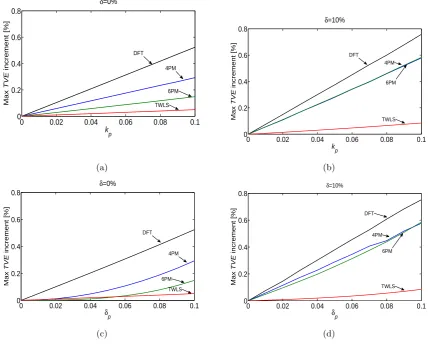
Fig. 3.3 shows the additional contributions to the maximum TVE values due to PM, after compensating the influence of the off-nominal frequency offsets. The lines in Fig. 3.3(a)-3.3(b) refer to different estimators and are plotted as a function of the modulation factor kp, for δ = 0% and δ = 10%, respectively, after setting δp = 0.1 in both cases.

(54)

0 0.02 0.04 0.06 0.08 0.1

0 0.2 0.4 0.6 0.8 k p Max TVE increment [%] δ=0% 6PM 4PM DFT TWLS (a)

0 0.02 0.04 0.06 0.08 0.1 0 0.2 0.4 0.6 0.8 k p Max TVE increment [%] δ=10% 6PM 4PM DFT TWLS (b)

0 0.02 0.04 0.06 0.08 0.1 0 0.2 0.4 0.6 0.8 δ_p Max TVE increment [%] δ=0% 6PM 4PM DFT TWLS (c)

0 0.02 0.04 0.06 0.08 0.1 0 0.2 0.4 0.6 0.8 δ_p Max TVE increment [%] δ=10% 6PM 4PM DFT TWLS (d)

Figure 3.3: Worst-case TVE increments as a function of different PM parameters forδ= 0% (a)-(c) and

δ= 10% (b)-(d). In (a) and (b)δp= 0.1, while in (c) and (d) kp= 0.1.

regardless of the amount of amplitude or phase modulations.

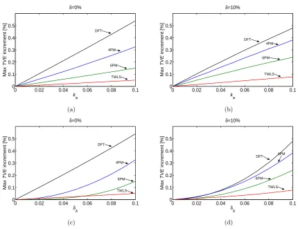
On the contrary, the TWLS estimator is more insensitive than the others to PM, while the influence of static frequency offsets and PM on the TVE are comparable. The results of the TVE sensitivity analysis to the AM parameters are shown in Fig. 3.4. The meaning of the curves and the values of the dual modulation parameters δa and ka is the same as those in Fig. 3.3. The trend of the various patterns and the related considerations are also quite similar. Even if the curves in Fig. 3.4(d) do not exhibit a linear behavior any longer, the DFT, 4PM, 6PM and TWLS estimators (in this order) have increasingly better performance in tracking possible AM fluctuations.

(55)

0 0.02 0.04 0.06 0.08 0.1 0 0.1 0.2 0.3 0.4 0.5 k a Max TVE increment [%] δ=0% 6PM 4PM DFT TWLS (a)

0 0.02 0.04 0.06 0.08 0.1 0 0.1 0.2 0.3 0.4 0.5 k a Max TVE increment [%] δ=10% 6PM 4PM DFT TWLS (b)

0 0.02 0.04 0.06 0.08 0.1 0 0.1 0.2 0.3 0.4 0.5 δ_a Max TVE increment [%] δ=0% 6PM 4PM DFT TWLS (c)

0 0.02 0.04 0.06 0