6
SCIENTIFIC HIGHLIGHT OF THE MONTH: ”First
principles calculation of Solid-State NMR parameters”
First principles calculation of Solid-State NMR parameters
Jonathan R. Yates1, Chris J. Pickard2, Davide Ceresoli1
1- Materials Modelling Laboratory, Department of Materials, University of Oxford, UK
2- Department of Physics, University College London, UK
Abstract
The past decade has seen significant advances in the technique of nuclear magnetic res-onance as applied to condensed phase systems. This progress has been driven by the devel-opment of sophisticated radio-frequency pulse sequences to manipulate nuclear spins, and by the availability of high-field spectrometers. During this period it has become possible to predict the major NMR observables using periodic first-principles techniques. Such calcula-tions are now widely used in the solid-state NMR community. In this short article we aim to provide an overview of the capability and challenges of solid-state NMR. We summarise the key NMR parameters and how they may be calculated from first principles. Finally we outline the advantages of a joint experimental and computational approach to solid-state NMR.
1
Introduction
Nuclear Magnetic Resonance (NMR) is, as the name implies, a spectroscopy of the nuclei in given material. Some nuclei (eg 1H, 13C, 29Si) are found to posses nuclear spin, and in the presence of a magnetic field exhibit small splittings in their nuclear spin states due to the Zeeman effect. Transitions between these levels are very much smaller than electronic excitations in the system and can be probed with radio-wave frequency pulses. At a first thought this might appear to only provide us with information about the nuclei; however, the precise splitting of the levels is found to be influenced by the surrounding electronic structure. This make NMR a highly sensitive probe of local atomic structure and dynamics.
For the case of a spin 1/2 nucleus the splitting is given byE =−γ~Bwhereγis the gyromagnetic ratio of the nucleus. To give a feel for the numbers involved we take the case of a hydrogen atom (for obvious reasons referred to as a proton by NMR spectroscopists) in the field of a typical NMR spectrometer (9.4 T). The separation of the nuclear spin levels is 2.65x10⁻²⁵
Figure 1: (right) 13C CP-MAS spectrum of a molecular crystal (Flurbiprofen(1)). The effect of magnetic shielding causes nuclei in different chemical environments to resonate at slightly different frequencies
can be increased by using high magnetic fields and choosing nuclei with a large value of γ. The largest commercially available solid-state NMR spectrometers operate at a field of 23.5 T (giving a Larmor frequency for protons of 1 GHz). However, the nuclear constants are dictated by nature and some common isotopes such as 12C or16O have no net spin, as will any nucleus with an even number of neutrons and protons. In many cases interesting and technologically significant elements have NMR active isotopes which are present in low abundance (eg Oxygen for which the NMR active 17O is present at 0.037%) and/or have small γ (eg 47Ti which has γ(47Ti)=0.06γ(1H) ). It is only with the latest techniques and spectrometers that NMR studies on such challenging nuclei has become feasible.
1.1 Solid-State NMR
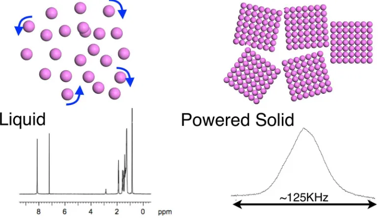
Figure 2: Schematic Representation of the difference between NMR on liquids and powered solids. In a solution the molecules tumble, leading to averaging of anisotropic interactions and sharp spectral lines. In a power the observed spectrum is now a superposition of all possible orientations, and anisotropic interactions lead to a broad spectrum.
information. On the other hand solid-state NMR has the potential to yield far more information than its solution-state counterpart. Anisotropic interactions can be selectively reintroduced into the experiment providing information on the principle components and orientations of the NMR tensors. The most widely used technique to reduce anisotropic broadening is Magic Angle Spinning (MAS). The magic angle,θ= 54.7◦
, is a root of the second-order Legendre polynomial (3cos2(θ)−1). For a sample spun in a rotor inclined at a fixed angle to the magnetic field, it can be shown that the anisotropic component of most NMR tensors when averaged over one rotor period, have a contribution which depends on the second-order Legendre polynomial. It follows that if the sample is spun aboutθ= 54.7◦
the anisotropic components will be averaged out (at least to first order). In practise this is achieved through the use of an air spin rotor, spinning speeds of 20kHz are common and the latest techniques allow for samples to be spun at up to 70kHz.
2
NMR parameters
There are a large number of NMR experiments ranging in complexity from a simple (one-dimensional) spectrum of a spin one-half nucleus such as13C, to sophisticated multidimensional spectra involving the transfer of magnetism between nuclear sites. All experiments depend on careful excitation, manipulation and detection of the nuclear spins. Several pieces of software have been developed to test NMR excitation sequences and to extract NMR parameters from experimental results (eg SIMPSON(2), Dmfit(3)). The correct language to describe this is that of effective nuclear Hamiltonians (see e.g. (4)). In a conceptual sense a spin Hamiltonian can be obtained from the full crystal Hamiltonian by integrating over all degrees of freedom except for the nuclear spins and external fields. The effect of the electrons and positions of the nuclei are now incorporated into a small number of tensor properties which define the key interactions in NMR. It is these tensors which can be obtained from electronic-structure calculations and we now examine them in turn.
2.1 Magnetic Shielding
The interaction between a magnetic field,Band a spin 1/2 nucleus with spin angular momentum ~IK is given by
H=−X K
γKIK·B. (1)
If we consider B as the field at the nucleus due to presence of an externally applied field Bext we can express Eqn. 1 as
H=−X K
γKIK(1 +←→σ k)Bext. (2)
The first term is the interaction of the bare nucleus with the applied field while the second accounts for the response of the electronic structure to the field. The electronic response is characterised by the magnetic shielding tensor←→σ K, which relates the induced field to the applied field
Bin(RK) =−←→σ KBext. (3)
In a diamagnet the induced field arises solely from orbital currentsj(r), induced by the applied field
Bin(r) = 1 c
Z d3r′
j(r′
)× r−r
′
|r−r′|3. (4)
The shielding tensor can equivalently be written as a second derivative of the electronic energy of the system
←→σ K=
∂2E ∂mK∂B
(5)
In solution state NMR, or for powdered solids under MAS conditions we are mainly concerned with the isotropic part of the shielding tensor σiso= 1/3T r[←→σ ]. The magnetic shielding results in nuclei in different chemical environments resonating at frequencies that are slightly different to the Larmor frequency of the bare nucleus. Rather than report directly the change in resonant frequency (which would depend of the magnetic field of the spectrometer) a normalised chemical shift is reported in parts per million (ppm)
δ= νsample−νref νref
where νref is the resonance frequency of a standard reference sample. The magnetic shielding and chemical shift are related by
δ = σref−σsample 1−σref
. (7)
For all but very heavy elements |σref| ≪1 and so
δ =σref−σsample. (8)
Figure 1 shows a typical 13C spectrum of a molecular crystal obtaining under MAS conditions. The spectrum consists of peaks at several different frequencies corresponding to carbon atoms in different chemical environments. The assignment has been provided by first-principles calcula-tion of the magnetic shielding. Strategies for converting between calculated magnetic shielding and observed chemical shift have been discussed in Ref. (5).
Calculations of magnetic shieldings have been implemented in several local-orbitals quantum chemistry code; see Ref (6) for an overview. For crystalline systems the GIPAW approach for computing magnetic shieldings(7; 8) was initially implemented in the PARATEC code. This is no longer developed but implementations are available in the planewave pseudopotential codes CASTEP(9; 10) and Quantum-Espresso (11). A method using localised Wannier orbitals(12) has been implemented in the planewave CPMD code. The CP2K program has a recent imple-mentation using the Gaussian and Augmented planewave method(13). In all these cases the shieldings are calculated using perturbation theory (linear response). Recently a method which avoids linear response, the so-called ‘converse approach’, have been developed (see Section3.2.2) and implemented in the Quantum-Espresso package.
2.2 Spin-spin coupling
In the previous section we considered the effect of the magnetic field at a nucleus resulting from an externally applied field. However, there may also be a contribution to the magnetic field at a nucleus arising from the magnetic moments of the other nuclei in the system. In an effective spin Hamiltonian we may associate this spin-spin coupling with a term of the form
H= X K<L
IK(DKL+JKL)IL. (9)
DKL is the direct dipolar coupling between the two nuclei and is a function of only the nuclear constants and the internuclear distance,
DKL =− ~
2πµ04πγKγL
3rKLrKL−1rL2 r5
KL
(10)
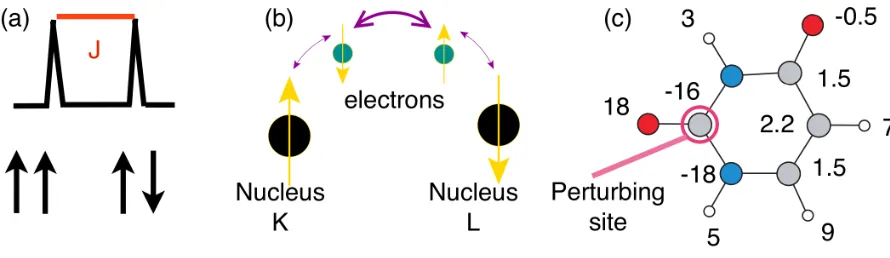
Figure 3: (a) Schematic representation of the effect of J coupling of two spin 1/2 nuclei on an NMR resonance. The peak is split by amount corresponding to the energy different between the spins being aligned parallel and antiparallel. (b) Schematic representation of the mechanism of transfer of J between nuclei. (c) Values of the J coupling (Hz) in Uracil (1H- white,13C - grey, 15N - blue,17O - red)
availability of high-field spectrometers that is has become possible to measure small J couplings (see Ref.(14) for a recent summary). Highlights have included the observation of two J couplings between a given spin pair(15), the measurement of distributions of J in amorphous materials(16), and reports of J as low as 1.5Hz(17)
The J-coupling is a small perturbation to the electronic ground-state of the system and we can identify it as a derivative of the total energy E, of the system
JKL=
~γKγL 2π
∂2E ∂mK∂mL
(11)
An equivalent expression arises from considering one nuclear spin (L) as perturbation which creates a magnetic field at a second (receiving) nucleus (K)
B(1)in (RK) = 2π
~γKγLJKL·mL. (12)
Eqn. 12 tells us that the question of computing J is essentially that of computing the magnetic field induced indirectly by a nuclear magnetic moment. The first complete analysis of this indirect coupling was provided by Ramsey(18; 19). When spin-orbit coupling is neglected we can consider the field as arising from two, essentially independent, mechanisms. Firstly, the magnetic moment can interact with electronic charge inducing an orbital currentj(r), which in turn creates a magnetic field at the other nuclei in the system. This mechanism is similar to the case of magnetic shielding in insulators. The second mechanism arises from the interaction of the magnetic moment with the electronic spin, causing an electronic spin polarisation. The relavant terms in the electronic Hamiltonian are the Fermi-contact (FC),
HFC =gβ µ0 4π
8π
3 S·µLδ(rL), (13)
and the spin-dipolar (SD),
HSD=gβµ0 4πS·
3rL(µL·rL)−rL2µL1 |rL|5
. (14)
magneton. The resulting spin densitym(r) creates a magnetic field through a second hyperfine interaction. By working to first order in these quantities we can write the magnetic field at atom K induced by the magnetic moment of atom L as
B(1)in (RK) = µ0 4π
Z
m(1)(r)·
3rKrK− |rK|2 |rK|5
d3r
+ µ0 4π
8π 3
Z
m(1)(r)δ(rK) d3r
+ µ0 4π
Z
j(1)(r)× rK |rK|3
d3r. (15)
Several quantum chemistry packages provide the ability to compute J coupling tensors in molec-ular systems (see Ref. (20) for a review of methods). An approach to compute J tensors within the planewave-pseudopotential approach has recently been developed(21). Some examples are discussed in Section 4.3, and a review of applications is provided in Ref. (22).
2.3 Electric Field Gradients
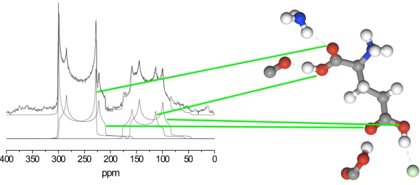
Figure 4: 17O NMR spectrum of Glutamic acid obtained using MAS. The upper trace is the ob-served spectrum, below is the deconvolution into four quadrupolar line-shapes. The assignment to crystallographic sites is provided by first principles calculation(23)
For a nucleus with spin >1/2 the NMR response will include an interaction between the quadrupole moment of the nucleus, Q, and the electric field gradient (EFG) generated by the surrounding electronic structure. The EFG is a second rank, symmetric, traceless tensor G(r) given by
Gαβ(r) = ∂Eα(r) ∂rβ
−1
3δαβ X
γ
∂Eγ(r)
∂rγ (16)
where α, β, γ denote the Cartesian coordinates x,y,z and Eα(r) is the local electric field at the position r, which can be calculated from the charge densityn(r):
Eα(r) = Z
d3r n(r)
|r−r′|3(rα−r ′
α). (17)
The EFG tensor is then equal to
Gαβ(r) = Z
d3r n(r) |r−r′
|3 "
δαβ −3
(rα−rα′)(rβ−rβ′) |r−r′
|2 #
The computation of electric field gradient tensors is less demanding than either shielding or J-coupling tensors as it requires only knowledge of the electronic ground state. The LAPW approach in its implementation within the Wien series of codes(24) has been widely used and shown to reliably predict Electric Field Gradient (EFG) tensors(25). The equivalent formalism for the planewave/PAW approach is reported in Ref. (26).
The quadrupolar coupling constant, CQand the asymmetry parameter,ηQcan be obtained from the the diagonalized electric field gradient tensor whose eigenvalues are labelled Vxx, Vyy, Vzz, such that|Vzz|>|Vyy|>|Vxx|:
CQ= eVzzQ
h , (19)
where h is Planck’s constant and
ηQ=
Vxx−Vyy Vzz
. (20)
The effect of quadrupolar coupling is not completely removed under MAS, leading to lineshapes which can be very broad. Figure 4 shows a typical MAS spectrum for a spin 3/2 nucleus. The width of each peak is related to CQ and the shape to ηQ. See Ref. (27) for recent review of NMR techniques for quadrupolar nuclei.
2.4 Paramagnetic Coupling
If a material contains an unpaired electron then this net electronic spin can create an additional magnetic field at a nucleus via Fermi contact and spdipolar mechanisms. Paramagnetism in-troduces several difficulties from the point of view of solid-state NMR, for example the resonances can exhibit significant broadening. However, NMR has been used to analyse local magnetic in-teractions, for example in manganites(28) and lithium battery materials(29). There are several reports of calculations of NMR parameters in paramagnetic systems for example paramagnetic shifts of 6Li(30) and EFGs of layered vanadium phosphates(31). However, to the best of our knowledge, unlike the case of paramagnetic molecules(32) there is currently no methodology to predict all of the relavant interactions in paramagnetic solids at a consistent computational level.
In metallic systems the electronic spin also plays an important role as the external field will create a net spin density (Pauli susceptibility) which will in turn create a magnetic field at the nucleus. This additional contribution to the magnetic shielding is known as the Knight shift. The linear-response GIPAW approach has been extended(33) to compute the magnetic shielding and Knight-shift in metallic systems, although there have been few applications to date.
3
A first principles approach
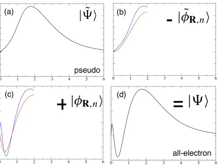
Figure 5: Schematic representation of the PAW transformation in Eqn. 21 using two projectors. The x-axis represents radial distance from a nucleus. (a) representation of the pseudowavefunc-tion (b) two pseudo-atomic like states (c) two corresponding all-electron atomic-like states (d) all-electron wavefunction.
3.1 Pseudopotentials
The combination of pseudopotentials and a planewave basis has proved to give a reliable de-scription of many material properties, such as vibrational spectra and dielectric response(10; 34), but properties which depend critically on the wavefunction close to the nucleus, such as NMR tensors require careful treatment. The now standard approach to computing such properties is the projector augmented wave method (PAW) introduced by Bl¨ochl(35) which provides a formalism to reconstruct the all-electron wavefunction from its pseudo counterpart, and hence obtain all-electron properties from calculations based on the use of pseudopotentials.
The PAW scheme proposes a linear transformation from the pseudo-wavefunction |Ψ˜i, to the true all-electron wavefunction |Ψi, ie|Ψi=T|Ψ˜i, where
T=1+X
R,n
[|φR,ni − |φ˜R,ni]hp˜R,n| (21)
|φR,ni is a localised atomic state (say 3p) and |φeR,ni is its pseudized counter part. |peR,ni are a set of functions which project out the atomic like contributions from |Ψ˜i. This equation is represented pictorially in Figure 5. For an all-electron local or semi-local operator O, the corresponding pseudo-operator, Oe, is given by
e
O =O+ X
R,n,m
As constructed in Eqn. 22 the pseudo-operator Oe acting on pseudo-wavefunctions will give the same matrix elements as the all-electron operator O acting on all-electron wavefunctions. Pseudo operators for the operators relavant for magnetic shielding are reported in Ref. (7; 8), for electric field gradients in Ref. (26) and for J coupling in Ref. (21). Pseudo-operators for magnetic shielding including relativistic effects at the ZORA level are given in Ref. (36)
For a system under a uniform magnetic field PAW alone is not a computationally realistic solution. In a uniform magnetic field a rigid translation of all the atoms in the system by a vector t causes the wavefunctions to pick up an additional field dependent phase factor, which can we written as, using the symmetric gauge for the vector potential, A(r) = 1/2B×r,
hr|Ψ′
ni=e i
2cr·t×Bhr−t|Ψ
ni. (23)
In short Eqn. 22 will require a large number of projectors to describe the oscillations in the wavefunctions due to this phase. In using a set of localized functions we have introduced the gauge-origin problem well known in quantum chemical calculations of magnetic shieldings(6). To address this problem Pickard and Mauri introduced a field dependent transformation operator
TB, which, by construction, imposes the translational invariance exactly:
TB=1+
X
R,n
e2icr·R×B[|φ
R,ni − |φ˜R,ni]hp˜R,n|e
−i
2cr·R×B. (24)
The resulting approach is known as the Gauge Including Projector Augmented Wave (GIPAW) method.
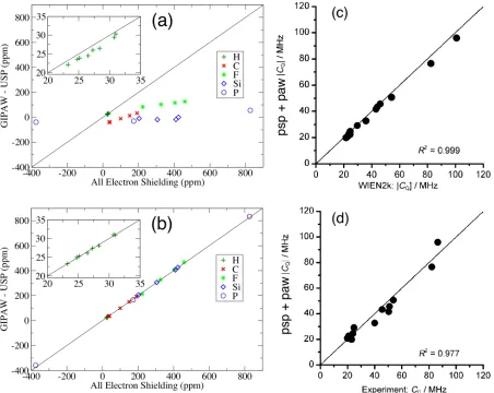
Figure 6: Comparison of all-electron and pseudopotential (with frozen core) calculations of NMR parameters. (a) Comparison of chemical shieldings for a range of small molecules computed using Guassian basis sets and those from pseudopotential calculations without the GIPAW augmenta-tion (b) as previous but using the GIPAW augmentaaugmenta-tion (c) Comparison of 93Nb Quadrupolar Couplings computed using peudopotentials and PAW with results from an LAPW+lo code (d) Results from previous as compared to experiment
3.2 Magnetic Response
3.2.1 Linear Response
As discussed in Section 2 one route to obtaining the magnetic shielding is to compute the induced orbital current,j(1)(r) using perturbation theory,
j(1)(r′
) = 4X o
RehhΨ(0)o |Jp(r′
)|Ψ(1)o ii+ 2X o
hΨ(0)o |Jd(r′
)|Ψ(0)o i. (25)
The current operator, J(r′
) is obtained from the quantum mechanical probability current, re-placing linear with canonical momentum. It can be written as the sum of diamagnetic and paramagnetic terms,
J(r′
) = Jd(r′
) +Jp(r′
), (26)
Jd(r′) = 1 cA(r
′
)|r′ihr′|, (27)
Jp(r′
) = −p|r
′
ihr′
|+|r′
ihr′
|p
The first-order change in the wavefunction|Ψ(1)o i, is given by
|Ψ(1)o i= X
e
|Ψ(0)e ihΨ(0)e | ε−εe H
(1)|Ψ(0)
o i=G(ε(0)o )H(1)|Ψ(0)o i, (29)
whereH(1)=p·A+A·p. Using the symmetric gauge for the vector potential,A(r) = (1/2)B×r, we arrive at the following expression for the induced current,
j(1)(r′
) = 4X o
RehhΨ(0)o |Jp(r′
)G(ε(0)o )r×p|Ψ(0)o ii− 1
2cρ(r
′
)B×r′
(30)
where ρ(r′
) = 2PohΨ(0)o |r′ihr′|Ψ(0)o i. For a finite system there is in principle no problem in computing the induced current directly from Eqn. 30. However, for an extended system there is an obvious problem with the second (diamagnetic) term of Eqn. 30; the presence of the position operator r will generate a large contribution far away fromr= 0, and the term will diverge in an infinite system. The situation is saved by recognising that an equal but opposite divergence occurs in the first (paramagnetic) term of Eqn. 30, and so only the sum of the two terms is well defined. Through the use of a sum-rule(7; 8; 40) we arrive at an alternative expression for the current
j(1)(r′
) = 4X o
RehhΨ(0)o |Jp(r′
)G(ε(0)o )(r−r′
)×p|Ψ(0)o ii. (31)
In an insulator the Green functionG(ε(0)o ) is localized and soj(1)(r′) remains finite at large values of (r−r′
). At this point there still remains the question of the practical computation of the current, which for reasons of efficiency it is desirable to work with just the cell periodic part of the Bloch function. Eqn. 31 is not suitable for such a calculation as the position operator cannot be expressed as a cell periodic function. One solution to this problem(40) is to consider the response to a magnetic field with a finite wavelength i.e. B=sin(q·r)ˆq. In the limit that q →0 the uniform field result is recovered. For a practical calculation this enables one to work with cell periodic functions, at the cost that a calculation at a point in the Brillouin Zonekwill require knowledge of the wavefunctions at k±q(ie six extra calculations for the full tensors for all atomic sites). A complete derivation was presented in Refs. (7; 40) leading to the final result for the current,
j(1)(r′
) = lim q→0
1 2q
S(r′
, q)−S(r′
,−q) (32)
where
S(r′
, q) = 2 cNk X i=x,y,z X o,k Re 1 ihu
(0) o,k|J
p
k,k+qi(r
′
)Gk+qi(εo,k)B×uˆi·(p+k)|u¯(0)o,ki
,
qi =quˆi,Nk is the number of k-points included in the summation and
Jpk,k+q
i =−
(p+k)|r′
ihr′
|+|r′
ihr′
|(p+k+qi)
2 . (33)
Equivalent expressions valid when using separable norm-conserving pseudopotentials are given in Ref. (7), and for ultrasoft potentials in Ref. (8).
3.2.2 Converse Approach
the macroscopic magnetization induced by magnetic point dipoles placed at the nuclear sites of interest. This method shall be referred to asconverse (41; 42) as opposed todirect approaches, based on linear-response, in which a magnetic field is applied and the induced field at the nucleus is computed.
The converse approach is made possible by the recent developments that have led to theModern Theory of Orbital Magnetization (43–47), which provides an explicit quantum-mechanical ex-pression for the orbital magnetization of periodic systems in terms of the Bloch wave functions and Hamiltonian, in absence of any external magnetic field.
The converse and linear response approaches should give the same shielding tensors if the same electronic structure method is used (eg the LDA). The main advantage of the converse approach is that it can be coupled easily to advanced electronic structure methods and situations where a linear-response formulation is cumbersome or unfeasible. For example in the case of DFT+U (48) or hybrid functionals, the converse method should provide a convenient shortcut from the point of view of program coding. It is possible that in the case of high-level correlated approaches like multi-configuration (49; 50) and quantum Monte Carlo, the converse method will also provide a convenient route to calculate NMR chemical shifts.
Let us start by considering a sample to which a constant external magnetic fieldBextis applied. The field induces a current that, in turn, induces a magnetic field Bind(r) such that the total magnetic field is B(r) = Bext +Bind(r). In NMR experiments the applied fields are small compared to the typical electronic scales; the absolute chemical shielding tensor ←→σ is then defined via the linear relationship
Bsind=−←→σ s·Bext, σs,αβ =− ∂Bs,αind
∂Bβext. (34)
The indexsindicates that the corresponding quantity is to be taken at positionrs, i.e., the site of nucleus s.
Instead of determining the current response to a magnetic field, we derive chemical shifts from the orbital magnetization induced by a magnetic dipole. Using Bs,α = Bαext+Bs,αind, Eq. (34) becomes δαβ −σs,αβ = ∂Bs,α/∂Bβext. The numerator may be written as Bs,α = −∂E/∂ms,α, where E is the energy of a virtual magnetic dipole ms at the nuclear position rs in the field
B. Then, writing the macroscopic magnetization as Mβ =−Ω−1
∂E/∂Bβ (where Ω is the cell volume), we obtain
δαβ−σs,αβ =− ∂ ∂Bβ
∂E ∂ms,α
=− ∂
∂ms,α ∂E ∂Bβ
= Ω ∂Mβ ∂ms,α
. (35)
In order to calculate the shielding tensor of nucleus susing eq. (35), it is necessary to calculate the induced orbital magnetization due to the presence of an array of point magnetic dipolesms at all equivalent sites rs. The vector potential of a single dipole in Gaussian units is given by
As(r) =
ms×(r−rs) |r−rs|3
. (36)
For an array of magnetic dipoles A(r) = PRAs(r−R), where R is a lattice vector. Since
A is periodic, the average of its magnetic field ∇ ×A over the unit cell vanishes; thus, the eigenstates of the Hamiltonian remain Bloch-representable. The periodic vector potentialA(r) can now be included in the Hamiltonian with the usual substitution for the momentum operator
p → p− ecA, where me is the electronic mass and c is the speed of light. Because of the lattice periodicity of the vector potential, the magnetic dipole interacts with all its images in neighboring cells. However, due to the 1/r3 decay of the dipole-dipole interaction, the chemical shifts are found to converge very fast with respect to super-cell size.
In practice, we can calculate the full shielding tensor by performing three SCF ground state calculations. In each SCF calculation, we place a virtual magnetic dipole ms(eq. (36)) aligned along one of the Cartesian directions and we calculate the resulting change in orbital magneti-zation.
The main disadvantage of the converse method is requires a set of three calculations for every atom we are interested in, as opposed to linear-response, which yield all the shielding tensors at once. This disadvantage can be partly mitigated by distributing every set of calculations on a large number of CPUs and machines. Of course, if we are interested on in a subset of atomic sites or atomic species, the converse method can be efficient as the linear-response approach.
In the case of a pseudopotential code the situation is complicated due to nonlocal projectors usually used in the Kleinman-Bylander separable form. However, by using the GIPAW formal-ism, the converse method has recently been generalized such that it can be used in conjunction with norm-conserving, non-local pseudopotentials, to calculate the NMR chemical shifts (51) and the EPR g-tensor (52).
The converse method has been recently implemented in Quantum-Espresso (11), VASP (53) and ADF-BAND (54).
4
Uses of Computations
4.1 NMR Crystallography
many supramolecular systems and organic compounds it is often not possible to obtain large single crystals. In such cases diffraction studies often provide only limited information eg just the unit cell parameters. However, the corresponding solid-state NMR spectra can show sharp peaks demonstrating that the material is locally well ordered. Here the challenge is to go di-rectly from NMR data to the crystal structure. NMR can also be used to probe dynamics in crystalline materials; a range of NMR experiments can be used to examine motion on differ-ent timescales(55). In all cases the ability to compute NMR observables from first-principles essential in order to provide the link between structure and spectra.
We examine some recent studies which highlight the interplay between diffraction, solid-state NMR and computations. An extensive list of applications of planewave/pseudopotential calcu-lations of NMR parameters can be found at http://www.gipaw.net.
4.1.1 Clinohumite - local disorder
Figure 7: (a) Crystal structure of Clinohumite showing the staggered arrangement of F/OH sites (grey). Atom colours are: Si (blue), Mg (green), O(red). (b) 19F MAS NMR spectrum of 50% fluorinated clinohumite. (c) Four possible local fluorine environments (d) Comparison of calculated 19F shielding and experimental shifts.
First-principles calculations and solid-state NMR have recently been used to study disorder in the fluorine substituted hydrous magnesium silicate clinohumite (4Mg2SiO4·Mg(F,OH)2). This mineral is of considerable interest as model for the incorporation of water within the Earth’s upper mantle. Diffraction provides the overall crystal structure but gives no information on the ordering of the F−
/OH−
environments. From these it was found that the computed 19F NMR parameters were clustered into four distinct ranges depending on their immediate neighbours. The ranges correspond well to the observed peaks providing an assignment of the spectrum. Interestingly further experiments revealed the presence of19F-19F J-couplings despite the fact that there is no formal bond between fluorine atoms. The magnitude of these coupling was reproduced by first-principles calculations, suggesting that there is a ‘though-space’ component to these J-couplings.
4.1.2 GexSe1−x glasses
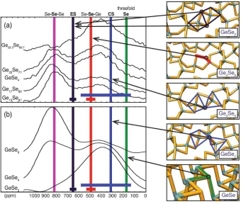
Figure 8: Average (vertical lines) and range (horizontal lines) of77Se chemical shifts as found for various Se sites in several crystalline precursors of Germanium Selenide glasses, together with experimental 77Se MAS spectra for GexSe1−x glasses.
Conventional diffraction studies do not provide sufficient information to determine the short range order in Chalcogenide GexSe1−x glasses, which can include corner-sharing, and
edge-sharing, tetrahedral arrangements, under-coordinated and over-coordinated atoms, and homopo-lar bonds. Recent 77Se NMR studies obtained under MAS have shown two large, but rather broad peaks (as shown in Figure 8). Two conflicting interpretations have been suggested: the first consists of a model of two weakly linked phases, one characterised by Se-Se-Se sites, the other Se-Ge-Se. The second model assumes a fully bonded structure with the contributions from Ge-Se-Se and Ge-Se-Ge linkages overlapping. To answer this question Kibalchenko et al(57) carried out first-principles calculations on several crystalline precursors of Germanium Selenide glasses (GeSe2, Ge4Se9 and GeSe) to establish the range of chemical shifts associated with each type of Se site. The results are summarised in Figure 8. This connection between local structure and observed NMR parameters provides a reliable interpretation of the 77Se spectra of GexSe1−x glasses, ruling out the presence of a bimodal phase and supporting a fully bonded
Charpentier and co-workers have used a combination of Monte Carlo and molecular dynamics simulations together with first-principles calculations of NMR parameters in order to parame-terise the relationship between local atomic structure and NMR observables. This methodology has been applied to interpret the NMR spectra of several amorphous materials including vitreous silica(58), calcium silicate glasses(59), lithium and sodium tetrasilicate glasses(60).
4.1.3 Structure Solution
A challenge for solid-state NMR is the idea of ‘NMR Crystallography’: the ability to go di-rectly from an observed NMR spectrum to the crystal structure(61). Early work by Facelli and Grant(62) combined calculation of 13C magnetic shieldings with single crystal NMR stud-ies. More recently proton-proton spin diffusion (PSD) experiments have been shown to provide three dimensional crystal structures which can be successfully used as input into a scheme for crystal structure determination. In Ref. (63) PSD measurements were combined with subse-quent DFT geometry optimisations to give the crystal structure of the small molecule thymol in good agreement with diffraction data. There has been considerable effort to develop schemes based on molecular modelling to predict the lowest energy polymorphs of molecular crystals. At the present time the best schemes are able to reliable predict the naturally occurring structure amongst a set of 10-100 low energy structures. Recent work has shown that the combination of computational and experimental 1H chemical shifts is sufficient to identify the experimental structure from amongst this set of candidate structures(64).
4.2 Dynamics and the role of temperature
NMR can be used to study motional processes in solids. One technique is the use of deuterium NMR.2H has spin I=2 and the magnitude of its quadrupolar coupling (typically 250kHz) makes it suitable to study motional processes on the micro and milli second timescale. Griffinet al(65) have used 2H solid-state NMR to study the dynamic disorder of hydroxyl groups in hydroxyl-clinohumite. In this material the deuteron can exchange between two crystallographic sites. By combining first-principles calculations, a simple model of the effect of motion on the NMR line-broadening, and experimental 2H NMR spectra it was possible to obtain the activation energy for the exchange processes.
NMR spectra are commonly obtained at room temperature. Given that first-principles calcula-tions are typically use a static configuration of atoms (eg obtained from diffraction) this raises questions about the influence of thermal motion on NMR spectra, even if it is thought that there are no specific motional processes, such as exchange, involved.
groups. In some cases it may be possible to quantify the effect of temperature experimentally. Webberet al(69) measured the change in1H and13C chemical shifts in the range 348 K to 248 K (by simply varying the temperature of the gas used inside the NMR probe). By extrapo-lating the results to 0K the change in 1H shift for the hydroxyl protons with respect to room temperature was 0.5ppm. The change in the C-H 1H shifts over the same range was less than 0.1ppm. The experimental shifts extrapolated to 0K were found to be in better agreement with first-principles calculation those those records at room temperature.
4.3 Experimental Design
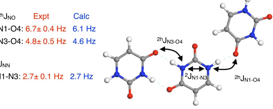
The ability to predict NMR observables allows the experimentalist to examine the feasibility of a particular NMR experiment, or optimise its setup (of course this implies that the experimentalist should trust the accuracy of the calculations!). One such area is the measurement of J-coupling in condensed phases. Current experiments can hope to observe values of J in organic compounds that are above about 5Hz. There is little empirical knowledge about magnitude of J couplings in solids, and so calculations have been used to identify systems with measurable couplings. An initial application of the planewave/pseudopotential approach for computing J-couplings in solids(70) showed that calculations at the PBE level gave values for 15N-15N J-couplings across hydrogen bonds in very good agreement with experimental measurements (typically within the experimental errors). The same study predicted that 13C-17O and 15N-17O J-couplings should be of sufficient magnitude to be observed experimentally. This prompted new experimental work on labelled samples of glycine.HCl and uracil. Further calculations were required to interpret the data resulting in the first experimental determination of the biologically significant13C-17O, 17O-17O and15N-17O J-couplings in the solid-state(71).
Figure 9: Calculated and Experimental J couplings in the crystalline form of Uracil
4.4 Improving First-principles methodologies
Reproduc-ing this data is a strict test of any first-principles methodology. In our experience, for a given geometry, both LDA and common GGA functionals (PBE, Wu-Cohen, PBEsol) give a very similar description of NMR parameters. Usually the agreement with experiment is reasonably good - a rough rule of thumb is that errors in the chemical shift are within 2-3% of the typi-cal shift range for that element. There are, however, some notable exceptions: Several groups have shown(56; 72) that while present functionals can predict the trends in19F chemical shifts, a graph of experimental against calculated shifts has slope significantly less than 1. Another example is the calculation of17O chemical shifts (73) in calcium oxide and calcium aluminosili-cates. There are significant errors in the17O shifts which arise due to the failure of GGA-PBE to treat the unoccupied Ca 3d states correctly. In Ref. (73) it was found that a simple empirical adjustment of the Ca 3d levels via the pseudopotential was sufficient to bring the 17O chemical shifts into good agreement with experiment. However, in both cases it is clear that current GGAs do not describe all of the relavant physics. The converse approach to computing NMR parameters provides an easy route to including exact-exchange in the calculation of magnetic shielding, and it will be interesting to see if this can improve the treatment of these known difficult cases.
5
Acknowledgements
We thank Dr. Mikhail Kibalchenko (EPFL), Dr. John Griffin (St Andrews) and Prof. John Hanna (Warwick) for providing figures.
References
[1] J. R. Yates et al., Phys. Chem. Chem. Phys. 7, 1402 (2005).
[2] M. Bak, J. T. Rasmussen, and N. C. Nielsen, J. Mag. Reson. 147, 296 (2000).
[3] D. Massiot et al., Magn. Reson. Chem. 40, 70 (2002).
[4] M. Levitt, Spin Dynamics (Wiley, Chicester, UK, 2002).
[5] R. K. Harris et al., Magn. Reson.in Chem.45, S174 (2007).
[6] Calculation of NMR and EPR Parameters. Theory and Applications, edited by M. Kaupp, M. B¨uhl, and V. G. Malkin (Wiley VCH, Weinheim, 2004).
[7] C. J. Pickard and F. Mauri, Phys. Rev B63, 245101 (2001).
[8] J. R. Yates, C. J. Pickard, and F. Mauri, Phys. Rev. B 76, 024401 (2007).
[9] S. J. Clark et al., Z. Kristall. 220, 567 (2005).
[10] V. Milman et al., J. Mol. Struct. THEOCHEM954, 22 (2010).
[11] P. Giannozzi et al., J. Phys.: Cond. Matter 21, 395502 (2009).
[12] D. Sebastiani and M. Parrinello, J. Phys. Chem. A105, 1951 (2001).
[14] D. Massiot et al., C.R. Chim. 13, 117 (2010).
[15] C. Coelho et al., Inorg. Chem. 46, 1379 (2007).
[16] P. Guerry, M. E. Smith, and S. P. Brown, J. Am. Chem. Soc.131, 11861 (2009).
[17] P. Florian, F. Fayon, and D. Massiot, J. Phys. Chem. C113, 2562 (2009).
[18] N. F. Ramsey and E. M. Purcell, Phys. Rev.85, 143 (1952).
[19] N. F. Ramsey, Phys. Rev.91, 303 (1953).
[20] T. Helgaker, M. Jaszunski, and M. Pecul, Progress in Nuclear Magnetic Resonance Spec-troscopy53, 249 (2008).
[21] S. A. Joyce, J. R. Yates, C. J. Pickard, and F. Mauri, J. Chem. Phys. 127, 204107 (2007).
[22] J.R.Yates, Magn. Reson. Chem. 48, S23 (2010).
[23] J. R. Yates et al., J. Phys. Chem. A108, 6032 (2004).
[24] P. Blaha, K. Schwarz, P. Sorantin, and S. Trickey, Comp. Phys. Comm. 59, 399 (1990).
[25] P. Blaha, P. Sorantin, C. Ambrosch, and K. Schwarz, Hyperfine Interact.51, 917 (1989).
[26] M. Profeta, F. Mauri, and C. J. Pickard, J. Am. Chem. Soc.125, 541 (2003).
[27] S. E. Ashbrook, Phys. Chem. Chem. Phys. 11, 6892 (2009).
[28] A. Trokiner et al., Phys. Rev. B74, 092403 (2006).
[29] C. P. Grey and N. Dupre, Chem. Rev.104, 4493 (2004).
[30] G. Mali, A. Meden, and R. Dominko, Chem. Commun.46, 3306 (2010).
[31] J. Cuny et al., Magn. Reson. Chem.48, S171 (2010).
[32] S. Moon and S. Patchkovskii, in Calculation of NMR and EPR Parameters: Theory and Applications, edited by V. M. M. Kaupp, M. Buhl (Wiley, Weinheim, 2004).
[33] M. d’Avezac, N. Marzari, and F. Mauri, Phys. Rev. B 76, 165122 (2007).
[34] S. Baroni, S. de Gironcoli, A. Dal Corso, and P. Giannozzi, Rev. Mod. Phys.73, 515 (2001).
[35] C. G. van de Walle and P. E. Bl¨ochl, Phys. Rev. B 47, 4244 (1993).
[36] J. R. Yates, C. J. Pickard, F. Mauri, and M. C. Payne, J. Chem. Phys. 118, 5746 (2003).
[37] T. Gregor, F. Mauri, and R. Car, J. Chem. Phys.111, 1815 (1999).
[38] J. V. Hanna et al., Chem. Eur. J.16, 3222 (2010).
[39] J. Cuny et al., ChemPhysChem10, 3320 (2009).
[40] F. Mauri, B. G. Pfrommer, and S. G. Louie, Phys. Rev. Lett. 77, 5300 (1996).
[42] T. Thonhauser, D. Ceresoli, and N. Marzari, Int. J. Quantum Chem. 109, 3336 (2009).
[43] R. Resta, D. Ceresoli, T. Thonhauser, and D. Vanderbilt, Chem. Phys. Chem. 6, 1815 (2005).
[44] T. Thonhauser, D. Ceresoli, D. Vanderbilt, and R. Resta, Phys. Rev. Lett. 95, 137205 (2005).
[45] D. Xiao, J. Shi, and Q. Niu, Phys. Rev. Lett.95, 137204 (2005).
[46] J. Shi, G. Vignale, D. Xiao, and Q. Niu, Phys. Rev. lett.99, 197202 (2007).
[47] D. Ceresoli, T. Thonhauser, D. Vanderbilt, and R. Resta, Phys. Rev. B 74, 024408 (2006).
[48] M. Cococcioni and S. de Gironcoli, Phys. Rev. B 71, 035105 (2005).
[49] E. Schreineret al., Proc. Natl. Acad. Sci.104, 20725 (2007).
[50] X. Deng, L. Wang, X. Dai, and Z. Fang, Phys. Rev. B79, 075114 (2009).
[51] D. Ceresoli, N. Marzari, M. G. Lopez, and T. Thonhauser, Phys. Rev. B81, 184424 (2010).
[52] D. Ceresoli, U. Gerstmann, A. P. Seitsonen, and F. Mauri, Phys. Rev. B81, 060409 (2010).
[53] F. Vasconcelos et al., private communication.
[54] D. Skachkov, M. Krykunov, E. Kadantsev, and T. Ziegler, J. Chem. Theory Comput. 6, 1650 (2010).
[55] Nuclear Magnetic Resonance Probes of Molecular Dynamics, edited by R. Tycko (Kluwer, Dordrecht, The Netherlands, 2003).
[56] J. M. Griffinet al., J. Am. Chem. Soc. 132, 15651 (2010).
[57] M. Kibalchenko, J. R. Yates, C. Massobrio, and A. Pasquarello, Phys. Rev. B 82, 020202 (2010).
[58] T. Charpentier, P. Kroll, and F. Mauri, J. Phys. Chem. C113, 7917 (2009).
[59] A. Pedone, T. Charpentier, and M. C. Menziani, Phys. Chem. Chem. Phys.12, 6054 (2010).
[60] S. Ispas, T. Charpentier, F. Mauri, and D. R. Neuville, Solid State Sci.12, 183 (2010).
[61] NMR Crystallography, edited by R. K. Harris, R. E. Wasylishen, and M. J. Duer (Wiley, Chichester, UK, 2009).
[62] J. C. Facelli and D. M. Grant, Nature365, 325 (1993).
[63] E. Salager et al., Phys. Chem. Chem. Phys. 11, 2610 (2009).
[64] E. Salager et al., J. Am. Chem. Soc. 132, 2564 (2010).
[65] J. M. Griffinet al., Phys. Chem. Chem. Phys. 12, 2989 (2010).
[66] J.-N. Dumez and C. J. Pickard, J. Chem. Phys. 130, 104701 (2009).
[68] C. Gervaiset al., Phys. Chem. Chem. Phys.11, 6953 (2009).
[69] A. L. Webber et al., Phys. Chem. Chem. Phys.12, 6970 (2010).
[70] S. A. Joyce, J. R. Yates, C. J. Pickard, and S. P. Brown, J. Am. Chem. Soc. 130, 12663 (2008).
[71] I. Hung et al., J. Am. Chem. Soc.131, 1820 (2009).
[72] A. Zheng, S.-B. Liu, and F. Deng, J. Phys. Chem. C113, 15018 (2009).