The modified probabilistic neural network as a nonlinear correlator detector

MURDOCH RESEARCH REPOSITORY

http://dx.doi.org/10.1109/ICNN.1995.488115

Zaknich, A. and Attikiouzel, Y. (1995) The modified probabilistic

neural network as a nonlinear correlator detector. In:

Proceedings., IEEE International Conference on Neural

Networks, 27 November - 1 December, Perth, Western

Australia, pp. 309 - 313.

http://researchrepository.murdoch.edu.au/18387/

Copyright © 1995 IEEE

Personal use of this material is permitted. However, permission to reprint/republish

this material for advertising or promotional purposes or for creating new collective

The Modified Probabilistic Neural Network as a Nonlinear Correlator

Detector

Anthony Zaknich, Member IEEE, Associate Member

of

AES

Yianni Attikiouzel, Senior Member IEEE, Fellow IEE, Fellow IEAust

Centre for Intelligent Information Processing Systems (CIIPS), Department of Electrical and Electronic Engineering,

The University of Western Australia, Nedlands 6907, Western Australia

Abstract

A Nonlinear correlator detector for the detection of a signal class with some intra class variance is developed using the Modified Probabilistic Neural Network and the General Regression Neural Network. An application, involving the detection of regular tone bursts transmitted over a poor and noisy radio channel subjected to fading, random noise and impulse noise effects, is used to show the effectiveness of the method as compared to a linear correlator.

The statistical dependency between two vector variables XI and x2 can be of t m types: linear

dependency or nonlinear dependency [I]. Linear dependency is what is normally regarded as correlation. If the variables are uncorrelated, they are no longer linearly dependent, but they may still be statistically dependent. Nonlinear dependency is called "residual" dependency because it is the dependency that remains after the linear dependency is removed. Two zero mean variables XI and x2 are uncorrelated if the expected value of their product is zero.

E[ XI x2 ] = 0, (uncorrelated)

But XI and x2 are independent if and only if their joint probability density function (pdf) is equal to the product of the individual densities.

p( XI, x2 ) = p( XI) p( x2 ), V XI and x2, (independent)

Therefore, it is possible for XI and x2 to be uncorrelated but still dependent. It is very useful to be able to assign the degree of dependency of a random variable to some specific process. This can apply to signal detection where the same process can generate a range of different signal waveforms rather than one specific waveform. This is typical in classical linear correlation, or matched filter detector systems. A complex example of this application is the detection and identification in time of a sheep's single chew from it's non deterministic jaw sound (This is a research problem that the authors are currently investigating in relation to sheep feeding studies). A simpler example is the accurate detection in time

of

deterministic signal codes transmitted over a radio channel which have been affected by various linear and nonlinear stochastic channel effects. These problems can be solved via a number of nonlinear signal detection techniques including statistical and neural network pattern recognition. However, these methods usually require sufficient training vectors available from the desired process together with the likely range of noise or non process signals to estimate a posteriori pdfs of each. Also, they are usually designed to test the hypothesis of signal present or absent rather than to give an accurate estimate of the signal location in time. It may be more convenient to have a nonlinear matching filter that works in a similar way to the correlator or optimal linear matching filter. In this case the signal presence would be determined by the output of the correlator exceeding a preset threshold and its location in time established by the position of the highest peak output as it is commonly done in the linear case.

defined to be p points long. An arbitrary vector x composed of p successive amplitude sample points from the process can be defined as:

x = [ x(n), x(n-I), x(n-2), ... x(n-p-I)

1,

n is the discrete time index.

The class waveform reference sample set can be specified as the vector set { xref i

I

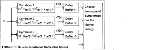
i = I , ... NUM }

and a general model for a nonlinear con-elator can be developed as shown in Figure 1.

energy

ll

FIGURE I: General Nonlinear Correlator Model

There are NUM parallel correlators with each of the Xref i being a correlator matching template. The correlation of vector x with each reference template IS then represented by (xTxref

,

). It is then normalised to one by dividing by (xTref i Xref i). The normalised output of each correlator is fed into a delay line 2p sample points long. The system output is taken from the output of the delay line which has the highest energy if it exceeds a minimum level, othervise the output is made zero. This introduces a system delay of 2p, so instead of taking the output of the highest energy delay line it would be acceptable to take the current input to that delay line instead. A neural network can be developed to embody this model and provide a continuous nonlinear correlator output r(x) as the vector x is taken from the process signal by sliding a sampling Andow p sample points long forward in time a point at a time.

The Modified Probabilistic Neural Network (MPNN) [2,3] and the General Regression Neural Netmrk (GRNN) [4] have an ideal architecture for this type of problem although any feed forward neural network can be used. Both these networks are related to the Probabilistic Neural Network (PNN) [5] which is normally considered to be a classifier but can also be used for non parametric pdf estimation. They can both be described as general regression or mapping functions given by:

NS

[Yi ~xP(-(E~)~(E~))I i = l 202

Y A W

=

NS

I ~ X P ( - ( E A S ~ ) ~ ( ~ - ~ ) ) I i = l 202

If the yi are allowed to have real scalar values equation (1) becomes exactly Specht's GRNN which incorporates each and every training vector pair {xi -> yi} into its architecture as does the PNN (xi is a single training vector in the input space and yi is the associated desired scalar output). If it can be assume that there is only one centre in the input space per output yi then a convenient general model

to use for all forms of the MPNN and the GRNN is: M

c

i = l 202

c

i = l 202

[ z i yi exp(-(x

-

centxi)T(x

-

centxi))

1

Y Y X ) = M

[ z i exp(-(x

-

centxi)T(x

-

centxi))

1

centxi is the centre or mean vector for class i in the input space (real valued or quantised). 0 is the single learning or smoothing parameter chosen during network training. Yi is the output related to centxi (real valued or quantised).

M is the number of unique centres i in the MPNN structure. Zi is the number of input training vectors Xj associated with centxi.

M NS = C

i = l

Equation (2) can be derived from the GRNN equation (1) through the following approximation: Zi, is the total number of training vectors.

Zi

j = 1

Zi exp-((x-centxi)T(x-centxi)/202)

c

~ x P - ( ( x - x ~ ) T ( x - x ~ ) / ~ ~ ~ ) (3)

This is a reasonable approximation if the Xj are close together in a relatively small local space and can be adequately represented by a single centre vector centxi. The key to the practical application of the general MPNN equation (2) is related to the method of selection of the yi and the grouping of the associated input vectors into the centre vector centxi for each class i. One solution to this selection and grouping for simple sinusoidal signals proposed by Zaknich et al [2] was to uniformly quantise the noiseless desired yi, separately group the y, having positive and negative slopes in the waveform and associate them with the mean of the input vectors mapping to each group. This simple case led to a more general approach, for both simple and more complex signals, of uniquely identifying the quantised yi having a similar local waveform pattern which was called the MPNN Method A [6]. Method A involved taking the desired waveform y(t) and uniformly sampling it in time to y(n) digital sample points which were then uniformly quantised into one of N quantisation levels to be able to define a desired output phase state vector composed of y(n) and the m-I quantised samples immediately preceding it in time, ie. (y(n), y(n-I), ....y( n-m-I). The greater the m the more uniquely a quantised output value y(n) or yi could be identified in the waveform for the purpose of associating all the input vectors Xi mapping into the same phase state. In most applications it was sufficient to use m = 1 with the y(n) sample quantised to one of N uniform levels and the y(n-I) to Ns levels (usually N = Ns but not necessarily).

The training of the GRNN and the MPNN Method A can be achieved by taking a long section of the process and identifying the exact p length window positions where the NUM class reference waveform vectors are located. A sequence of training vectors x, can be collected by starting at the beginning and sliding one point at time through the whole training signal. The training set of {input -> output} vector pairs are created as follows:

<xj -> (XjTXref i ) / (Xref iTxref i)

1

j

=

I

,...

NS

1

if xj overlaps Xref j, else {xj ->

o

I

j

=

I ,... NS

1,

assuming only one Xref i overlaps with Xj at a time.

After the GRNN or MPNN has been trained and optimised it produces the normalised linear correlation output with respect to nearest matching template to the input vector x. Therefore, although the templates may not be linearly dependent they are non linearly dependent and this dependence becomes quantified by the nonlinear correlator output values r(x). After training this nonlinear correlator can be used for the detection of class vectors if the output exceeds a preset detection threshold 9 and their location in time by their peak output.

An application based on the detection of regular tone bursts transmitted over a poor and noisy radio channel was contrived to test the MPNN/GRNN Nonlinear Correlator described above. It was

assumed that the tone frequency, amplitude fading and phase effects were unknown and were considered to be normal intra-class variations. Only the burst length was fixed and known. This application tested the Nonlinear Correlator for signal detection and location in time and it was compared with the best linear correlator solution since there was significant linear correlation between the tone bursts. The variable tone burst signal in this case can be thought of as a deterministic signal with some intra-class variance due to the fading effects plus random zero mean white noise and impulse noise.

points of the input signal which included the current sample point x(n) and the 29 sample points immediately prior to it, ie.

x

=

[x(n),x(n-~ ),x(n-2) ,... .

.

...

. .

,x(n-p-l )IT, vector.

FIGURE 2: 640 polnts of testlng signal and dested output

The data sets used in this application were as follows: training data, NS = 710, p = 30, K = 1, delay = 0. testing data, NS = 710, p = 30, K = 1, delay = 0.

FIGURE 3: Llnea ColTetata Output for the Testlng Slgnal Input

Figure 2 shows the testing input or source signal and the desired or normalised nonlinear correlator output signal. The training signal pair

was

another independent signal pair which looked very similar to the testing signal pair. All the peak nonlinear correlator outputs were 1.0.

1

The peak outputs of the desired normalised correlation output all had the same amplitude according to the nonlinear correlator model defined above. When the source signal

was

passed through a linear correlator with a matching template made from a 18 ms long sine burst, having a frequency of 400 Hz and constant amplitude the waveform s h o w in Figure 3 resulted. The peak output

was

0.8380 which

was

less than the maximum possible value of 1.0. The individual peak amplitudes varied according to the varying amplitudes of the tones in the source signal which were subject to the fading effects. A similar output was achieved when the source signal

was

filtered by a 30 tap finite impulse response (FIR) filter trained with the same training data. This FIR filter actually became a linear correlator so it

was

no surprise that its output and performance

was

very similar.

81.95 seconds

The times in the tables are obtained using Borland C 3.0 implementations on an 80486 PC running at 33 MHz, and they are quoted for reference only. A GRNN

was

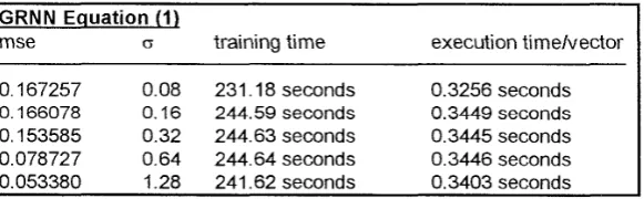
trained to implement the nonlinear correlator and the following results were achieved.

GRNN Equation (1)

mse cs training time execution timelvector

0.167257 0.08 231.18 seconds 0.3256 seconds 0.166078 0.16 244.59 seconds 0.3449 seconds 0.153585 0.32 244.63 seconds 0.3445 seconds 0.078727 0.64 244.64 seconds 0.3446 seconds 0.053380 1.28 241.62 seconds 0.3403 seconds

Training for both the GRNN and MPNN usually involves the selection of a single optimal parameter (5

which gives the minimum mean square error (mse) between the desired correlator outputs and the actual netmrk outputs as the whole testing set of data is passed through the netwark. The training data set is incorporated into the netmrk architecture, either directly as for the GRNN or indirectly as

for the MPNN. In this case the mse approached a minimum as cr -> 00 but it resulted in a degenerate

solution. As 0 -> CO the output approached a constant output irrespective of the input x. The mse

measure therefore,

was

not an appropriate one for this problem. It

was

better to seek a minimum absolute error between the output and the desired response. It

was

more important to ensure that the peak outputs remained close to 1.0 rather than let them degenerate for the sake of an overall low

mse. Considering the nature of the mapping, it would be best to seek the response of the nearest training vector to x. This implies that a lower CJ which produced more

of

a nearest neighbour solution nd the MPNN). A c

=

0.16

was

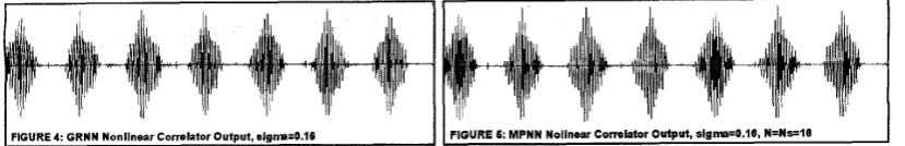
chosen even though the mse ed the best output waveform with the peaks at the right height latively higher than expected mainly due to the fact that there were relatively few training vectors compared to the possible variety that they could achieve from that process.

FIGURE 4: GRNN Nonlinear Comhtor Output, elgm:0.16 FIGURE 5: MPNN Nollnoar Comelator Output, slgm=O.l6, N=Ns=18

I

The peak output achieved by passing the testing signal through the GRNN was 0.9998 which showed it

was

working correctly. Another benefit of the GRNN result

was

that the gap noise

was

quite

low,

lower in fact than that present in the training data, as can be seen in Figure 4. This indicated that the GRNN

was

providing some extra beneficial noise smoothing.

The MPNN Method A implementation of the nonlinear correlator gave similar results as for the GRNN, as can be seen in Figure 5, but with a smaller or more efficient network size. It provided more noise smoothing as expected. The peak output from the testing signal

was

0.9997. The results for a few different quantisation selections were as follows.

Data MPNN Method A, Equation (2).

m=2

M N Ns mse C training time execution time per vector

403 32 32 0.166718 0.16 139.67 secs 0.19672 seconds 249 16 16 0.167216 0.16 86.29 secs 0.12153 seconds 117 8 8 0.166750 0.16 40.59 secs 0.0571 7 seconds

Conclusions

Both the GRNN and MPNN Method A produced better results than the linear method and thus demonstrate their suitability for the intended class of signal detection applications. The method would be more effective if more training vectors were used but there

was

sufficient evidence to indicate that the method was valid.

Makhoul, J., Roucos, S . and Gish,

H.,

"Vector quantisation in speech coding", Proceedings of the IEEE, Vol. 73, No. 11, November 1985, pp. 1551-1588.

Zaknich, Anthony, desilva, Christopher and Attikiouzel, Yianni, 'The probabilistic neural netmrk for nonlinear time series analysis", IEEE International Joint Conference on Neural Networks (IJCNN), Singapore, 17-2ISt November 1991, pp. 1530-1535.

Zaknich, Anthony and Attikiouzel, Yianni, "Automatic optimization of the modified probabilistic neural network for pattern recognition and time series analysis", Proceedings of the First Australian and New Zealand Conference on Intelligent Information Systems, Perth, Western Australia, 1-3rd December, 1993, pp. 152-156.

Specht, D. F., "A general regression neural network", IEEE Transactions on Neural Networks, Vol. 2, No. 6, November 1991, pp. 568-576.