Second Order Learning Algorithm for Back Propagation Neural Networks

(1)

Vol.7 (2017) No. 4

ISSN: 2088-5334

Second Order Learning Algorithm for Back Propagation Neural

Networks

Nazri Mohd Nawi

#

, Noorhamreeza Abdul Hamid

#

, Noor Azah Samsudin

#

, Mohd Amin Mohd Yunus

#

,

Mohd Firdaus Ab Aziz

#

Faculty of Computer Science and Information Technology, Universiti Tun Hussein Onn Malaysia, 86400, Johor, Malaysia E-mail: [email protected]

Abstract— Training of artificial neural networks (ANN) is normally a time-consuming task due to iteratively search imposed by the

implicit nonlinearity of the network behavior. In this work an improvement to ‘batch-mode’ offline training methods, gradient-based or gradient free is proposed. The new procedure computes and improves the search direction along the negative gradient by introducing the ‘gain’ value of the activation functions and calculating the negative gradient on an error with respect to the weights as well as ‘gain’ values in minimizing the error function. The main advantage of this new procedure is that it is easy to implement into other faster optimization algorithms such as conjugate gradient method and Quasi-Newton method. The performance of the proposed method implemented into conjugate gradient method and Quasi-Newton method is demonstrated by comparing the simulation results to the neural network toolbox for the chosen benchmark. The simulation results clearly demonstrate that the proposed method significantly improves the convergence rate significantly faster the learning process of the general back propagation algorithm because of it new efficient search direction.

Keywords— Back propagation algorithm; gradient descent; activation function; second order method; search direction

I. INTRODUCTION

Methods to speed up and optimize the learning process in feed forward neural networks (MLFNN) have been recently studied and several new adaptive learning algorithms have been discovered. The most popular learning algorithm is the batch Back-propagation (BP) [1], [2] and it is the most common and widely used supervised training algorithm in solving a large number of classification and function interpolation problems. BP algorithms are based on the gradient descent algorithm which is well known in optimization theory, and they usually exhibit poor convergence rate and depend on parameters which have to be specified by the user, because no theoretical basis for choosing them exists [3]. The choices of selecting the best values for those parameters are often crucial for the success of the algorithm and definitely required the designer to arbitrarily select parameters such as initial weights and biases, a learning rate value, activation function, network topology and gain of the activation function. It has been found that very small variations in these values can make the difference between good, average or bad performance [4]. This is also the main reason why the BP algorithm is too slow, and generalization is not always good.

Many studies have been done to improve back propagation learning algorithm, and those studies fall roughly into two categories. The first category involves the development of ad hoc techniques [5]-[6], [7]-[14]. In this technique some of them introduced the momentum term, others used the alternative cost function or dynamic adaptation of the learning parameters. Many apply special techniques of initialization of weights.

Another category of research has focused on standard numerical optimization technique [15]-[17]. The most popular approaches from the second category have used conjugate gradient or quasi-Newton (Secant) methods. The quasi-Newton methods are considered to be more efficient, but their storage and computational requirements go up as the square of the size of the network.

(2)

Among those improvements, the researches focusing on using ‘gain’ parameter are among the easiest to implement. The gain parameter controls the steepness the activation function. A few researchers hypothesized about the existence of a relationship between gain of the activation function and the weights [21]-[22] or between the gain and learning rate [1], [3], [23]-[24], and Zurada [25] showed that using activation functions with large gains yield results similar to those with a high learning rate.

In this paper, we demonstrate that by changing the gain of the activation functions in the gradient descent algorithm it is actually improving the search direction and not the learning rate. The motivation of this research is that changing the gain activation functions is very effective means for improving the search direction in general back propagation. Later on, we implement and evaluate the effect of adaptive gain value on the well-known non-linear conjugate gradient algorithm and Quasi-Newton methods.

This research starts by initiating the basic iterations of those optimisation methods in the form of w_r+1=w_r +λ_rd_r where d_r is a descent search direction and λ_r is a learning rate obtained by one-dimensional search. In the conjugate gradient methods, it considers the search direction as

1

)

( + −

−∇

= r r r

r E w d

d β , where the scalar β_r is chosen in such manner that the method reduces to the linear conjugate gradient when the function is quadratic, and the line search is exact. The rest of methods define the search direction by

) (

1 r r

r B Ew

d =− −∇ where B is a nonsingular symmetric _r matrix. Mainly, the matrix B is selected as: _r Br =I(the steepest descent method), 2 ( )

r

r E w

B =∇ (the Newton’s method) or an approximation of the Hessian 2 ( )

r

w E

∇ (BFGS,

DFP, etc.).

In this paper, we are not a concern on how to determine the learning rate because our main interest is in finding the efficient search direction in order to improve the learning.

By applying the new procedure in calculating an efficient search direction, this paper presents two improved learning algorithm which is conjugate gradient with Fletcher Reeves update (CGFR-AG) and Broyden-Fletcher-Goldfarb-Shanno (BFGS-AG) method for back propagation neural networks. The proposed approaches presented in the paper consist of three steps: (1) Modification of standard back propagation algorithm by introducing gain value of the activation function, (2) Calculating the gradient descent on error with respect to the weights and gains values and (3) the determination of the new search direction with the function of gain variation.

In order to verify the efficacy of the proposed method, we perform simulation experiments on four selected benchmark problems. The remaining of the paper is organised as follows: In Section II we proposed our modification on standard back propagation algorithm with gain variation and validate the proposed algorithm with ‘sine curve’ example [26]. Some discussion of the proposed modification on Conjugate gradient with Fletcher Reeves update (CGFR-AG) and the Broyden-Fletcher-Goldfarb-Shanno (BFGS-AG) algorithm with new search direction procedure is presented in Section III. Experiments and simulation results are presented in

Section IV. The final section contains concluding remarks and short discussion for further research.

II. MATERIAL AND METHOD

The standard back propagation algorithm has become the most popular algorithm used for training multi-layer feed forward network. In this paper, the training will be referring to batch training of the multi-layer perceptron (MLP) and can be formulated as a nonlinear unconstrained optimization problem. The objective of a learning process is to find a

weight vector

w

which minimizes the different between the actual output and the desired output. Namely,

) (

min

Ew

n

w∈ℜ

(1)

Suppose for a particular input pattern

o

0 and let the input layer is layer 0. The desired output is the teacher

pattern

t

=

[

t

₁

...

t

_n

]

T, and the actual output is

o

_kL, where L denotes the output layer. Define an error function on that pattern as,

∑

−

= _k L

k

k o

t

E 2

) ( 2

1 ₍₂₎

The overall error on the training set is simply the sum, across patterns, of the pattern error

E

. The main purpose of the training is to search an optimal set of connection weights so that the errors of the network output can be minimized.

Let s k

o be the activation of the

k

thnode of layer s , and let

T s n s s

o

=

[

1

...

]

be the column vector of the activation values

in the layer s and the input layer as layer 0. Let

w

_ijsbe the weight on the connection from the

i

thnode in layer s−1 to the

j

thnode in layer s , and let

w

s_j

=

[

w

₁s_j

...

w

_njs

]

T be the column vector of weights from layers−1to the

j

thnode of layer s . The net input to the

j

thnode of layer s is defined

as

=

−

=

∑

−

k s k s

k j s

s j s

j

w

o

w

o

net

(

,

1

)

_, 1 , and let

T s n s

s

_net

net

=

[

₁

...

]

be the column vector of the net input values in layer s . The activation of a node is given by a function of its net input,

)

(

sj

s j s

j

f

c

net

o

=

(3)

where _f is any function with bounded derivative, and

s j

c

is a real value called the gain of the node.

In neural network training, an activation function is used for limiting the amplitude of the output of a neuron to generates an output value for a node in a predefined range as the closed unit interval c or alternatively [-1, +1]. In this paper, we use a common choice of activation function of the neurons in multilayer neural network, which is the logistic or sigmoid activation function. For the

_j

th_{node in layer s ,}

s j s jnet

c s

j

e

o ₋

+ =

1

1 ₍₄₎

(3)

(

)

_j

k s k s

k j s

j

w

o

net

=

∑

−1

+

θ

, (5)

where

θ

_jis a bias for the

j

th unit and

c

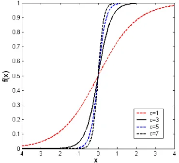
s_j is a real value called the gain of the activation function.

In general the value of the gain parameter,c , directly

influences the slope of the activation function [27]. For large gain values (

c

>>1), the activation function approaches a ‘step function’ whereas for small gain values (0 <

c

<< 1), the output values change from zero to unity over a large range of the weighted sum of the input values and the sigmoid function approximates a ‘linear function’ as shown in Fig. 1.

Fig. 1 The effect of gain on sigmoid activation function

To simplify the calculation, taken from the Equation (2) we then can perform gradient descent on E with respect to

w

_ijs. The chain rule yields

s ij s j s j s j s j s s

s

ij w

net net

o o net net

E w

E

∂ ∂ ∂

∂ ∂ ∂ ∂

∂ = ∂

∂ +

+ . . .

1 1

1 1 1 1

1 ... ]. . '( ) .

[ −

+ +

  

 

  

  − −

= s

j s j s j s j s

nj s j s n s

o c net c f

w w

M

δ

(6)

where

s j s

j

net E

∂ ∂ − =

δ

. In particular, the first three factors of (6)

indicate that

∑

+ +

=

k

s j s j s j s

j k s k s

c net c f

w ) '( )

( 1

, 1

1

δ

(7)

The iterative Equation (7) for s 1

δ

is the same as standard back propagation [4] except for the appearance of the value gain. By combining (6) and (7) yields the learning rule for weights:

1 −

=

∆

s

j s j s

ij

o

w

λδ

(8) where

λ

is a small positive constant called ‘step length’ or ‘learning rate’.

Gradient descent on error with respect to the gain can also be calculated by using the chain rule as previously described; it is easy to compute as

s j s j s j k

s j k s k s

j

net net c f w c

E

) ( ' )

( ,1

1

∑

+ +

= ∂

∂

_δ

₍₉₎

Then,

s j s j s j s j

c net c =

λδ

∆ (10)

The learning rule for gains (10) is easily incorporated into standard back propagation algorithms.

As in the standard back propagation algorithm uses the gradient descent search direction with a fixed step length

λ

in order to perform the minimization of the error function. The iterative form of this algorithm is:

r r

r

w

₊₁

=

+

∆

(11) where

r r

r d

w =λ

∆ and

r

d is the search direction or gradient

vector of the error function

E

at

r

w . Let

r r

w E d

δ δ

−

= and

d

_r

=

g

_r.

It is well known that pure gradient descent methods with fixed step length tend to be inefficient [28] due to the fact that the choose of search directions and step sizes are not optimal, if the first step size does not lead directly to the minimum, gradient descent will zig-zag with many small steps leading to very long computation times.

In order to avoid the oscillation, Rumelhart et. al. [4] modified the back propagation search direction (d ) by adding momentum term (

α

):

)

(

₁

1

1 + −

+

=

−

r

+

r r

−

r

g

w

d

α

(12)

Although this extra term can avoid the oscillation, it will introduce another extra term that has to be considered. In our next section, we will show that by adding the momentum term (α ) is wise when the values

λ

and α are well chosen by using conjugate gradient method.

Previous researches [1], [3], [4] claimed that the adaptive gain variation improved the learning rate or in order words, it improved the step length as they referred Equation (7) and (8) in calculating weight update expression with gain variation as:

1 1

, 1

)

(

'

)

(

∑

+ + −

=

∆

s

j k

s j s j s j s

j k s k s

ij

w

f

c

net

c

o

w

λ

δ

(13)

λ

*

c

s_j

Previous researchers assumed that by coupling gain and learning rate in Equation (13) it would improve the learning rate automatically and as a result, the algorithm converge faster as illustrated in Fig. 2.

r

(4)

This paper will show in our simulation results that the contribution of the adaptive gain value in Equation (13) is much more where it is actually improving the search direction and not the step length as shown in Fig. 3.

We will show in our simulation results that the contribution of the adaptive gain value in Equation (13) is actually improving the search direction and not the step length as shown in Fig. 3.

Fig. 3 Actual improvement on search direction by adaptive gain variation

As we note from Equation (6) and (7), the proposed back propagation produces the new search direction with the new procedure in calculating gradient with respect to weights and gain value. In order to increase the convergence speed by using this new gradient information, we propose to use conjugate gradient and the Broyden-Fletcher-Goldfarb-Shanno (BFGS) algorithm with this new search direction. In the sequel, we present the modified of conjugate gradient and the Broyden-Fletcher-Goldfarb-Shanno (BFGS) algorithm.

A. Validation on Sine Curve Example

The proposed approach was validated on a standard feedforward neural network with one hidden layer by having five hidden nodes. The training data set was created by using the function

y

=

x

+

sin(

2 *

π

*

x

),

where

x

∈

[

0 ,

1 ]

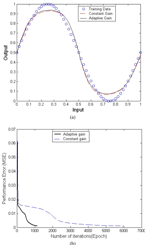
as been suggested by Bishop [24]. The network is trained using 0.3 as the learning rate value to achieve a target error equal to 0.001. The batch mode training was employed in training the Gradient Descent algorithm with adaptive changes in weight, bias and gain values. The initial weight and bias values were chosen as small random numbers in the range [-1, +1]. The network is trained with an adaptive gain with an initial value of unity for the gain parameter for all output as well as hidden nodes.

In Fig. 4(a) the network output (continuous curve) is shown against the training data points (circles)

)

*

2 sin(

x

y

=

+

π

. The output of the network using constant unit gain value is also plotted in Fig. 4(a) (dotted curve). Again, the result showed that the speed of convergence is high due to the modified gain values. As

shown in Fig. 4(b), the network required 1154 epochs to achieve the target error using the proposed adaptive gain algorithm in batch mode, whereas using the same set of initial weight and biases the network required 6014 epochs to achieve the target error using constant unit gain value during training.

Comparing both the curves in Fig. 4(a) it can be seen that the training performance of the adaptive gain algorithm is similar to that using constant gain value. However, the speed of convergence of the adaptive gain algorithm is very high as compared to that using constant gain value as shown in Fig. 4(b). The results proved that there is a dramatic improvement in the learning speed of the back-propagation algorithm.

(a)

(b)

Fig. 4 Output of the neural network training to learn a sine curve with and without using the adaptive gain in back propagation algorithm (a), and convergence speed for the sine function with and without using the adaptive gain algorithm in back propagation training (b)

Next section, in order to confirm the claim in the previous section, by means of simulation, this paper demonstrated the implementation of the proposed method which used gradient information with adaptive gain into the Broyden-Fletcher-Goldfarb-Shanno (BFGS).

λ

r

g

s j

c

*

λ

Fig. 2 New step length with adaptive gain variation claimed by previous researchers [1]-[3]

λ

)

(

_r r

c

g

r

(5)

B. Broyden-Fletcher-Goldfarb-Shahno (BFGS/AG) Algorithm with the Proposed New Search Direction Procedure

While BP is a steepest descent algorithm, the Broyden-Fletcher-Goldfarb-Shanno (BFGS) algorithm [28]-[29] is an approximation to Newton's method. Suppose that we have an

error function

E

(w

)

which we want to minimize with respect to the parameter vector

w

, then the search direction

d for Newton’s method is found by solving the system of equations

) ( )] (

[ 2E w 1 E w

d =−∇ − ∇ (14)

where ∇2E(w)=H is the Hessian matrix and ∇E(w)=g. This method converges in one iteration for a quadratic function. Unfortunately, it needs the computation of the inverse of Hessian matrix. This becomes a very difficult task for real applications. The BFGS algorithm allows constructing 2 ( )

w E

∇ by using the only gradient information with the function of gain value

) ( )

(w g c

E =

∇ provided in Section II. The complete algorithm works are shown as follows:

Step 1: Initializing the vector )

0 (

w and a positive definite

initialization of Hessian

matrix_H₍₀₎. Select a

convergence thresholdCT.

Step 2: Compute the descent search

directiond_r

dr =−Hrgr(cr)

Step 3: Search the optimal value

for *

r

λ by using line search

technique such as: ) (

min ) (

0 *

r r r r

r

r d E w d

w

E λ λ

λ +

= +

≥

Step 4: Update_w_r:

w_r w_r *_rd_r

1= −λ

+

Step 5: Compute _s_r=_w_r₊₁−_w_r

yr =gr+1(cr+1)−gr(cr)

r T r

r T r r r T r

T r r r T r

r r T r r

y s

H y s y s

s s y s

y H y

−

   

 

+ =

∇ 1

Step 6: Update the inverse

matrixH_r:

_H_r₊₁=_H_r +∇_r

Step 7: Compute the error function valueE(wr)

Step 8: If E(wr)>CTgo to Step 2, else stop training

C. Conjugate Gradient-Fletcher Reeves (CGFR/AG) Algorithm with the Proposed New Search Direction Procedure

One of the main reason for choosing conjugate gradient method because of its known and remarkable properties in generating in a very economical fashion, a set of vectors with a property known as conjugacy [26]. The standard

conjugate gradient method is an unconstrained optimization technique used to minimize the nonnegative error function

E

(w

)

by generating a sequence of approximation

w

_r₊₁iteratively according to:

r r r

r

w

d

w

₊1

=

+

λ

(15)

The scalar

λ

_r is the step length, known in neural network notation as learning rate. As we mentioned earlier, we are

not a concern in finding the optimal step length

λ

_rbecause it can be determined by many line search techniques in the way that

f

(

w

_r

+

λ

_r

d

_r

)

is minimized along the directiond_r, given

w

_r and d_r fixed. We focused on finding the optimal search direction as in the standard conjugate gradient algorithm; it begins the minimization process with an initial estimatew and an initial search ₀

direction as:

r r

r

g

w

E

d

=

−

=

δ

(16)

With adaptive gain variation the calculation for a new search direction with the function of gain is:

)

(

)

(

_k_,_r _r _k_,_r

r

c

g

c

w

E

d

=

−

=

δ

(17)

As for standard conjugate gradient, each direction d_r₊₁is

chosen to be a linear combination of the gradient descent direction −g_r₊₁and the previousd_r. As written as:

r r r

r

g

d

₊₁

=

−

₊₁

+

β

(18)

With adaptive gain, we calculated each new direction

1 +

r

d

as:

) ( ) ( )

( , 1 , ,

1

1 kr r kr r kr

r

r c c d c

w E

d

β

δ

+

−

= +

+

+ (19)

where the scalar

β

_r is to be determined by the requirement

that

d

_rand

d

_r₊₁must fulfil the conjugacy property. There are many formulae for the parameter

β

_r. One of them is introduced by Fletcher and Reeves [28] and is given as:

r T r

r T r r

g

₊₁ ₊₁

=

β

(20)

The complete CGFR-AG algorithm works as indicated in the following algorithm:

Step 1: Initializing the weight vector

0

w randomly, the gradient

vector ₀

0 =

g and gain

vectorc0=1. Let the first

search direction_d₀=_g₀.

Set

β

0 =0,

epoch

=

1

andr=1.

(6)

weight parameters. Select a

convergence thresholdCT.

Step 2: At step

r

, evaluate

gradient vector _g_r₍_c_r₎ with

respect to gain vectorc_r.

Step 3: EvaluateE(wr). If E(wr)<CT

then STOP training ELSE go to Step 4.

Step 4: Evaluate search direction:

1 1

)

( + ₋ ₋

−

= r r r r

r g c d

d

β

Step 5: For the first iteration,

check if r>1 THEN update

)

(

)

(

)

(

)

(

₁ ₁ ₁

1 1

r r r T r

r r r T r r

c

g

c

g

c

g

c

g

₊ ₊ ₊ ₊

+

=

β

ELSE go

to step 6.

Step 6: If

[(

epoch

+

1 )

/

Nt

]

=

0

THEN ‘restart’ the gradient vector with d_r =−g_r₋₁(c_r₋₁) ELSE go to Step 7.

Step 7: Calculate the search the

optimal value for λ*_rby using

line search technique such as:

) (

min ) (

0 *

r r r r

r

r d E w d

w

E +λ = _λ +λ

≥

Step 8: Updatew_r:

_w_r _w_r *_r_d_r

1= −λ

+

Step 9: Evaluate new gradient

vector gr+1(cr+1) with respect to gain value_c_r₊₁.

Step 10: Evaluate new search direction:

r r r r r

r g c c d

d+1 =− +1( +1)+β ( )

Step 11: Set r=r+1 and go to Step 2.

Conjugate gradient algorithm established much faster convergence rate than first-order gradient descent approach. This is because Conjugate Gradient uses its second order convergence property without complex calculation of the Hessian matrix.

Conjugate gradient method relies on improved gradient descent search direction. Later we showed that with an adaptive gain in Conjugate Gradient method had improved further the search direction. As a result, it converges faster.

III.RESULTS AND DISCUSSION

A computer simulation has been developed to evaluate the performance of the proposed the learning algorithms. The simulations have been carried out on a Pentium IV 3 GHz PC Dell with 1 GB RAM and using MATLAB version 6.5.0 (R13).

Six selected benchmark datasets were used as datasets as suggested by Prechelt [30] in order to study and evaluated the performance of the algorithm. Those six classification problems are 7-bit parity problem, Thyroid, Wisconsin breast cancer, Diabetes, Iris classification problem and glass classification problem.

For the purposes of comparison, all algorithms were trained by using the same networks architecture and

parameters setting for the same problem. Furthermore, the performances of all the proposed algorithms are also compared with respect to the neural network toolbox. For each problem, five algorithms have been analysed. The first algorithm is standard back propagation (BP), second Broyden-Fletcher-Goldfarb-Shanno (trainbfg) from ‘Matlab Neural Network Toolbox version 4.0.1’. The other two algorithms are standard Broyden-Fletcher-Goldfarb-Shanno (BFGS) and our proposed Broyden-Fletcher-Goldfarb-Shanno (BFGS) method with adaptive gain (CGFR/AG).

Since some of the values for parameters in Toolbox were set to default, therefore, both algorithms from Toolbox and proposed algorithm were fixed with the values of learning rate = 0.3, momentum term = 0.7 and standard sigmoid activation function is used for all nodes in the network. The gain parameters of all nodes are set to 1.0 initially. For all simulations, all algorithms were tested using the same initial weights, initialized randomly from the range [0, 1] and received the same sequence of input patterns.

All results were presented as a table which summarizes the performance of the algorithms for simulations that have reached a solution. All algorithms were trained with 100 trials, if an algorithm fails to converge, it is considered that it fails to train the FNN, but its epochs, CPU time and generalization accuracy are not included in the statistical analysis of the algorithms.

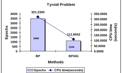
A. Thyroid Problems

This dataset was one of the famous datasets and was created based on the ‘artificial neural network’ version of the ‘thyroid disease’ problem dataset from the UCI repository of machine learning databases. The main objective of the dataset is trying to diagnose thyroid hyper or hypo-function based on patient query data and patient examination data in order to decide whether the patient’s thyroid has over-function, normal function or under-function. For a standard experiment, the selected architecture of the FNN is 21-5-3. The target error for this datasets is set to 0.05 with the maximum epochs is 1000.

Tyroid Problem

321.2350

111.6042

0 500 1000 1500 2000 2500 3000 3500 4000

BP BP/AG

Methods

E

p

o

c

h

s

0.0000 50.0000 100.0000 150.0000 200.0000 250.0000 300.0000 350.0000

C

P

U

t

im

e

(s

e

c

o

n

d

s

)

Epochs CPU time(seconds)

3469

1104

Fig. 5 The comparison of the number of epochs and CPU time needed to convergence for BP and BP/AG for thyroid problem

As can be seen in Fig. 5, the proposed method with adaptive gain had reduced three times number of CPU time and epochs as compared to the standard BP. In Fig. 6,

the

(7)

compared to traincgf, yet with the introduction of gain in the proposed method, the number of CPU time and the number of epochs had been reduced significantly. Same results can be seen in Fig. 7 where the proposed BFGS/AG outperformed both algorithms with up to 33% faster.

Tyroid Problem

9.9072

6.4269

4.7710

0 10 20 30 40 50 60

traincgf CGFR CGFR/AG

Methods

E

p

o

c

h

s

0.0000 2.0000 4.0000 6.0000 8.0000 10.0000 12.0000

C

P

U

ti

m

e

(s

e

c

o

n

d

s

)

48

15 11

Fig. 6 The comparison of the number of epochs and CPU time needed to convergence for traincgf, CGFR and the proposed CGFR/AG for thyroid problem

Tyroid Problem

8.6648

9.6249

5.2678

0 10 20 30 40 50 60 70

trainbfg BFGS BFGS/AG

Methods

E

p

o

c

h

s

0.0000 2.0000 4.0000 6.0000 8.0000 10.0000 12.0000

C

P

U

ti

m

e

(s

e

c

o

n

d

s

)

62

35 62

21

Fig. 7 The comparison of the number of epochs and CPU time needed to convergence for trainbfg, BFGS and the proposed BFGS/AG for thyroid problem

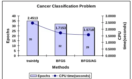
B. Wisconsin Breast Cancer Classifications Problems This dataset was created based on the ‘breast cancer Wisconsin’ problem and was taken from UCI repository of machine learning databases. It was created by Dr. William H. Wolberg [31], where Dr. William tried to diagnose breast cancer by trying to classify a tumor as either benign or malignant based on cell descriptions gathered by microscopic examination. For this problem, the selected architecture of the FNN is 9-5-2 and the target error was set as to 0.02 with the maximum epochs is 1000.

It can be seen from Fig. 8 that the effect of the proposed adaptive gain into back propagation had reduced the CPU time and number of epochs up to 38%. In addition in Fig. 9, the standard CGFR performed slightly better as compared to traincgf, however, the proposed CGFR/AG had reduced further the number epochs until 60%. Overall, Fig. 10 demonstrated that the proposed method BFGS/AG outperformed others algorithms in term of CPU time and number of epochs.

Cancer Classification Problem

52.1555

18.7154

0 200 400 600 800 1000 1200

BP BP/Ag

Methods

E

p

o

c

h

s

0.0000 10.0000 20.0000 30.0000 40.0000 50.0000 60.0000

C

P

U

ti

m

e

(s

e

c

o

n

d

s

)

1109

425

Fig. 8 The comparison of the number of epochs and CPU time needed to convergence for BP and the proposed BP/AG for cancer classification problem

3.7883

3.3060

1.5503

0 10 20 30 40 50 60 70 80

Methods

E

p

o

c

h

s

0.0000 0.5000 1.0000 1.5000 2.0000 2.5000 3.0000 3.5000 4.0000

C

P

U

ti

m

e

(s

e

c

o

n

d

s

)

71

65

39

Fig. 9 The comparison of the number of epochs and CPU time needed to convergence for traincgf, CGFR and the proposed CGFR/AG for cancer classification problem

2.4513

1.7153

1.5718

0 5 10 15 20 25 30 35 40

Methods

E

p

o

c

h

s

0.0000 0.5000 1.0000 1.5000 2.0000 2.5000 3.0000

C

P

U

ti

m

e

(s

e

c

o

n

d

s

)

35

32 ₂₉

Fig. 10 The comparison of the number of epochs and CPU time needed to convergence for trainbfg, BFGS and the proposed BFGS/AG for cancer classification problem

C. Diabetes Classifications Problems

This dataset was taken from the UCI repository of machine learning database and was created based on the ‘Pima Indians diabetes’ problem dataset. The datasets, doctors try to diagnose diabetes of Pima Indians based on personal data (age, the number of times pregnant) and the results of medical examinations (e.g. blood pressure, body mass index, the result of glucose tolerance test, etc.) before deciding whether a Pima Indian individual is diabetes positive or not. Again, the selected architecture of the FNN is for this datasets is 8-5-2 where the target error is set to 0.01, and the maximum epochs are 1000.

(8)

CPU time as compared to the standard BP as shown in Fig. 11. Same results can be seen in Fig. 12 and 13 where the proposed method CGFR/AG and BFGS/AG had outperformed other algorithms in term of CPU time and a number of epochs.

Diabetes Classification Problem

26.0133

14.7113

0 100 200 300 400 500 600

BP BP/AG

Methods

E

p

o

c

h

s

0.0000 5.0000 10.0000 15.0000 20.0000 25.0000 30.0000

C

P

U

ti

m

e

(s

e

c

o

n

d

s

)

517

413

Fig. 11 The comparison of the number of epochs and CPU time needed to convergence for BP and the proposed BP/AG for diabetes classification problem

4.0060

2.6000

2.0030

0 20 40 60 80 100 120

Methods

E

p

o

c

h

s

0.0000 0.5000 1.0000 1.5000 2.0000 2.5000 3.0000 3.5000 4.0000 4.5000

C

P

U

ti

m

e

(s

e

c

o

n

d

s

)

97

50

40

Fig. 12 The comparison of the number of epochs and CPU time needed to convergence for traincgf, CGFR and the proposed CGFR/AG for diabetes classification problem

4.1166

4.6721

4.0448

0 20 40 60 80 100 120

Methods

E

p

o

c

h

s

3.6000 3.8000 4.0000 4.2000 4.4000 4.6000 4.8000

C

P

U

ti

m

e

(s

e

c

o

n

d

s

)

106 95 ₈₃

Fig. 13 The comparison of the number of epochs and CPU time needed to convergence for trainbfg, BFGS and the proposed BFGS/AG for diabetes classification problem

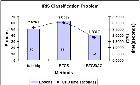
D. IRIS Classifications Problems

This is perhaps the best-known database to be found in the pattern recognition literature a classical classification dataset and was made famous by Fisher [32]. The datasets try to illustrate principles of discriminant analysis. Fisher's paper is considered as a classic paper in the field and is frequently

referenced to this day. The best-selected architecture of the FNN for this problem is 4-5-3 where target error was set as 0.05, and the maximum epochs was set to 1000.

Fig. 14 shows that the proposed implementation on BP/AG had significantly improved the convergence time as compared to the standard BP in term of CPU time and number of epochs. It is clear that the proposed method CGFR/AG and BFGS/AG had outperformed other algorithms in term of CPU time and a number of epochs as can be seen in Fig. 15 and Fig. 16.

IRIS Classification Problem

28.8065

21.7131

0 100 200 300 400 500 600 700 800

BP BP/AG

Methods

E

p

o

c

h

s

0.0000 5.0000 10.0000 15.0000 20.0000 25.0000 30.0000 35.0000

C

P

U

ti

m

e

(s

e

c

o

n

d

s

)

743

587

Fig. 14 The comparison of the number of epochs and CPU time needed to convergence for BP and the proposed BP/AG for IRIS classification problem

3.8071

1.9146

1.4232

0 10 20 30 40 50 60 70 80

Methods

E

p

o

c

h

s

0.0000 0.5000 1.0000 1.5000 2.0000 2.5000 3.0000 3.5000 4.0000

C

P

U

ti

m

e

(s

e

c

o

n

d

s

)

69

39

29

Fig. 15 The comparison of the number of epochs and CPU time needed to convergence for traincgf, CGFR and the proposed CGFR/AG for IRIS classification problem

2.6267

3.0063

1.8317

0 10 20 30 40 50 60 70

Methods

E

p

o

c

h

s

0.0000 0.5000 1.0000 1.5000 2.0000 2.5000 3.0000 3.5000

C

P

U

ti

m

e

(s

e

c

o

n

d

s

)

50 63

40

(9)

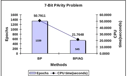
E. 7 BIT Parity

The parity problem is also one of the classical and considers the most popular initial testing tasks that are very demanding for classification particularly for the neural network to solve. This is because the target-output always changes whenever a single bit in the input vector changes and this makes generalization difficult, and as a result, the learning does not always converge easily [33]. For this problem, the selected architecture of the FNN is 7-5-1, where the target error has been set to 0.05 with the maximum epochs is set to 3000.

In achieving the target error, the performance of the proposed method BP/AG had significantly reduced the number of epoch up to 50% as shown in Fig. 17. Whereas, in Fig. 18 and 19 the proposed CGFR/AG and BFGS/AG still maintain the ability to reach the target error with a slight improvement in term of CPU time and the number of epochs.

7-Bit PArity Problem

50.7911 21.7648 0 200 400 600 800 1000 1200 1400 1600 BP BP/AG Methods E p o c h s 0.0000 10.0000 20.0000 30.0000 40.0000 50.0000 60.0000 C P U ti m e (s e c o n d s )

Epochs CPU time(seconds) 1339

545

Fig 17 The comparison of the number of epochs and CPU time needed to convergence for BP and the proposed BP/AG for 7-Bit parity problem

7-Bit Parity Problem

10.6129 10.6496 8.1057 0 50 100 150 200 250 300

Methods E p o c h s 0.0000 2.0000 4.0000 6.0000 8.0000 10.0000 12.0000 C P U t im e (s e c o n d s )

Epochs CPU time (seconds)

273

147

114

Fig. 18 The comparison of the number of epochs and CPU time needed to convergence for traincgf, CGFR the proposed CGFR/AG for 7-Bit parity problem

7-Bit Parity problem

4.4451 4.0183 3.7330 0 20 40 60 80 100 120 140 160 180

Methods E p o c h s 3.2000 3.4000 3.6000 3.8000 4.0000 4.2000 4.4000 4.6000 C P U t im e (s e c o n d s )

Epochs CPU time(seconds) 164

93

85

Fig. 19 The comparison of the number of epochs and CPU time needed to convergence for trainbfg, BFGS the proposed BFGS/AG for 7-Bit parity problem

F. Glass Classification Problem

This dataset was also taken from the UCI repository of machine learning database. The dataset was created based on the ‘glass’ problem where it was based on the study to classify types of glass and was motivated by the criminological investigation. From the study, the results of a chemical analysis of glass splinters (percent content of 8 different elements) plus the refractive index are used to classify the sample to be either float processed or non-float processed building windows, vehicle windows, containers, tableware, or head lamps. The problem contains 9 inputs, 6 outputs, 214 examples and the selected architecture of the FNN is 9-5-6, where the target error has been set to 0.05 with the maximum epochs is set to 3000.

Glass Classification Problem

32.9061 20.4352 0 100 200 300 400 500 600 700 800 BP BP/AG Methods E p o c h s 0.0000 5.0000 10.0000 15.0000 20.0000 25.0000 30.0000 35.0000 C P U ti m e (s e c o n d s )

698

492

Fig. 20 The comparison of the number of epochs and CPU time needed to convergence for BP and the proposed BP/AG for glass classification problem

6.5244 9.6080 5.6083 0 50 100 150 200 250 300

Methods E p o c h s 0.0000 2.0000 4.0000 6.0000 8.0000 10.0000 12.0000 C P U ti m e (s e c o n d s )

277

108

72

Fig. 21 The comparison of the number of epochs and CPU time needed to convergence for traincgf, CGFRS the proposed CGFR/AG for glass classification problem

3.9691 2.3268 0.9285 0 20 40 60 80 100 120 140

Methods E p o c h s 0.0000 0.5000 1.0000 1.5000 2.0000 2.5000 3.0000 3.5000 4.0000 4.5000 C P U ti m e (s e c o n d s )

116

27 ₁₅

(10)

Fig. 20 demonstrated that the proposed BP/AG had improved the performance of reaching the target error by reducing the number of epochs up to 30%. Again, the proposed CGFR/Ag and BFGS/AG outperformed other algorithms in reaching the target error as can seen in Fig. 21 and 22.

IV.CONCLUSION

In this paper, a new and improved training method is introduced for fast supervised learning method in the neural network. The performance of the proposed first order and second order methods with adaptive gain (BP-AG, CGFR-AG, BFGS-AG) with standard second order methods without gain (BP, CGFR, BFGS) in terms of speed of convergence evaluated in the number of epochs and CPU time. Based on some simulation results, it’s showed that the proposed algorithm had shown improvements in the convergence rate with 40% faster than other standard algorithms without losing their accuracy. It has been shown that the proposed algorithm is also robust as the results have been compared with the ‘Matlab neural network toolbox ‘implementation. Based on simulation results on selected benchmark datasets, the results clearly show that the proposed method outperforms the standard training algorithms in neural network toolbox. Furthermore, it runs much faster, performs less CPU time, has improved average number of epochs, and better convergence rates without losing their accuracy performance.

ACKNOWLEDGMENT

The authors would like to thank Universiti Tun Hussein Onn Malaysia (UTHM) Ministry of Higher Education (MOHE) Malaysia for financially supporting this Research under Trans-disciplinary Research Grant Scheme (TRGS) vote no. T003. This research also supported by GATES IT Solution Sdn. Bhd under its publication scheme.

REFERENCES

[1] Thimm G., Moerland F., and Emile Fiesler, The Interchangeability of Learning Rate an Gain in Back propagation Neural Networks. Neural Computation, 1996. 8(2): p. 451-460.

[2] Chin Kim On, Teo Kein Yau, Rayner Alfred, Jason Teo, Patricia Anthony, Wang Cheng, Backpropagation Neural Ensemble for Localizing and Recognizing Non-Standardized Malaysia’s Car Plates. International Journal on Advanced Science, Engineering and Information Technology, Vol. 6 (2016) No. 6, pages: 1112-1119. [3] Eom K. and Jung K., Performance Improvement of Back propagation

algorithm by automatic activation function gain tuning using fuzzy logic. Neurocomputing, 2003. 50: p. 439-460.

[4] Holger R. M. and Graeme C. D., The Effect of Internal Parameters and Geometry on the Performance of Back-Propagation Neural Networks. Environmental Modeling and Software, 1998. 13(1): p. 193-209.

[5] Rumelhart D. E., Hinton G. E., and Williams R. J., Learning internal representations by back-propagation errors. Parallel Distributed Processing, 1986. 1 (Rumelhart D.E. et al. Eds.): p. 318-362. [6] Sotiropoulos D.G., Kostopoulos A.E., and G. T.N., A spectral

version of Perry's Conjugate gradient method for neural network training. 4th GRACM Congress on Computational Mechanics (GRACM 2002), 2002. 1: p. 291-298.

[7] Weisss and Kulikowski, Computer systems that learn. 1991: p. 223.

[8] Fahlman S.E., Faster learning variations of back propagation: An empirical study. D. Touretzky, G.E. Hinton and T.J. Sejnowski (editors) Proceedings of the1988 Connectionist Models Summer School, 1988: p. 38-51.

[9] Hollis P. W., Harper J. S., and Paulos J. J., The Effects of Precision Constraints in a Backpropagation Learning Network. Neural Computation, 1990. 2(3): p. 363-373.

[10] Jacobs R.A., Increased rates of convergence through learning rate adaptation. Neural Networks, 1988. 1: p. 295–307.

[11] Kamarthi S. V. and Pitner S., Accelerating Neural Network Training using Weight Extrapolations. Neural Networks, 1999. 12: p. 1285-1299.

[12] Leonard J. and Kramer M. A., Improvement to the backpropagation algorithm for training neural networks. Computer and Chemical Engineering, 1990. 14(3): p. 337-341.

[13] Looney C. G., Stabilization and Speedup of Convergence in Training Feed Forward Neural Networks. Neurocomputing, 1996. 10(1): p. 7-31.

[14] Perantonis S. J. and Karras D. A., An Efficient Constrained Learning Algorithm with Momentum Acceleration. Neural Networks, 1995. 8(2): p. 237-249.

[15] Tollenaere T., SuperSAB: Fast adaptive back propagation wiih good scaling properties. Neural Networks, 1990. 3(5): p. 561-573. [16] Rigler A. K., Imine J. M., and Vogl T. P., Rescaling of variables in

hack propagation learning. Neural Networks, 1990. 3(5): p. 561-573. [17] Yusuf Hendrawan, Dimas Firmanda Al Riza, Machine Vision

Optimization using Nature-Inspired Algorithms to Model Sunagoke Moss Water Status. International Journal on Advanced Science, Engineering and Information Technology, Vol. 6 (2016) No. 1, pages: 45-57.

[18] Shanno D.F., Recent advances in numerical techniques for large scale oprimization. in Neural Nelworks for Control. Miller. Sutton and Werbos, 1990.

[19] Charalambous C., Conjugate gradient algorithm for efficient training of artificial neural networks. IEEE Proc, 1992. 139(3): p. 301-310. [20] Douglas S. C. and Meng T. H.-Y., Linearized least-squares training

of multilayer feedforward neural networks. IEEE lnternational]oint Conference on Neural Networks, 1991. 1: p. 1307-1312.

[21] Wessels L. F. A. and Barnard E., Avoiding false local minima by proper initialization of connections. IEEE Transactions on Neural Networks, 1992. 3: p. 899-905.

[22] Codrington C. and Tenorio M., Adaptive Gain networks. Proceedings of the IEEE International Conference on Neural Networks (ICNN94), 1994. 1: p. 339-344.

[23] Noriega, L., Multilayer Perceptron Tutorial. Lecture notes, 2005: p. 1-12.

[24] Holger R. Maier and Graeme C. Dandy, The effect of internal parameters and geometry on the performance of back-propagation neural networks: an empirical study. Environmental Modelling & Software, 1997. 13: p. 193-209.

[25] Zurada J.M., Introduction to Arti4cial Neural Systems. 1992, St. Paul, MN: West Publishing Company.

[26] Bishop C. M., Neural Networks for Pattern Recognition. 1995: Oxford University Press.

[27] Tai-Hoon Cho, Richard W. Conners, and Philip A. Araman, Fast Back-Propagation Learning Using Steep Activation Functions and Automatic Weight Reinitialization. IEEE International Conference on Systems, Man, and Cybernetics, 1991. 3: p. 1587-1592.

[28] Adrian J. Sheperd, Second Order Methods for Neural Networks-Fast and Reliable Training Methods for Multi-layer Perceptrons, ed. J.G. Taylor. 1997: Springer. 143.

[29] Byatt D., Coope I. D., and PriceC. J., E ect of limited precision on the BFGS quasi-Newton algorithm. ANZIAM J, 2004. 45: p. 283-295.

[30] 28. Fletcher R. and Reeves R. M., Function minimization by conjugate gradients. Comput. J., 1964. 7(2): p. 149-160.

[31] L.Prechelt, Proben1 - A set of Neural Network Bencmark Problems and Benchmarking Rules. Technical Report 21/94, 1994: p. 1-38. [32] Mangasarian O. L. and W.W. H., Cancer diagnosis via linear

programming. SIAM News, 1990. 23(5): p. 1-18.