Stability and conservation properties of transient field simulations using FIT

c

Copernicus GmbH 2003

Advances in

Radio Science

Stability and conservation properties of transient field simulations

using FIT

R. Schuhmann and T. Weiland

Technische Universit¨at Darmstadt, Dept. of Electrical Engineering and Information Technology, Computational Electromagnetics Laboratory (TEMF), Schloßgartenstr. 8, 64289 Darmstadt, Germany

Abstract. Time domain simulations for high-frequency applications are widely dominated by the leapfrog time-integration scheme. Especially in combination with the spatial discretization approach of the Finite Integration Technique (FIT) it leads to a highly efficient explicit simulation method, which in the special case of Cartesian grids can be regarded to be computationally equivalent to the Finite Difference Time Domain (FDTD) algorithm. For stability reasons, however, the leapfrog method is restricted to a maximum stable time step by the well-known Courant-criterion, and can not be applied to most low-frequency applications. Recently, some alternative, unconditionally stable techniques have been proposed to overcome this limitation, including the Alternating Direction Implicit (ADI)-method. We analyze such schemes using a transient modal decomposition of the electric fields. It is shown that stability alone is not sufficient to guarantee correct results, but additionally important conservation properties have to be met.

Das Leapfrog-Verfahren ist ein weit verbreitetes Zeit-integrationsverfahren f¨ur transiente hochfrequente elek-trodynamischer Felder. Kombiniert mit dem r¨aumlichen Diskretisierungsansatz der Methode der Finiten Integra-tion (FIT) f¨uhrt es zu einer sehr effizienten, expliziten Simulationsmethode, die im speziellen Fall kartesischer Rechengitter als ¨aquivalent zur Finite Difference Time Domain (FDTD) Methode anzusehen ist. Aus Sta-bilit¨atsgr¨unden ist dabei die Zeitschrittweite durch das bekannte Courant-Kriterium begrenzt, so dass das Leapfrog-Verfahren f¨ur niederfrequente Probleme nicht sinnvoll angewendet werden kann. In den letzten Jahren wurden alternativ einige andere explizite oder “halb-implizite” Zeit-bereichsverfahren vorgeschlagen, u.a. das “Alternating Di-rection Implicit” (ADI)-Verfahren, die keiner Beschr¨ankung des Zeitschritts aus Stabilit¨atsgr¨unden unterliegen. Es zeigt

Correspondence to: R. Schuhmann, T. Weiland

(schuhmann/[email protected])

sich aber, dass auch diese Methoden im niederfrequenten Fall nicht zu sinnvollen Simulationsergebnissen f¨uhren. Wie anhand einer transienten Modalanalyse der elektrischen Felder in einem einfachen 2D-Beispiel deutlich wird, ist die Ursache daf¨ur die Verletzung wichtiger physikalischer Er-haltungseigenschaften durch ADI und verwandte Methoden.

1 Introduction

Especially in high-frequency field simulations, where one of-ten deals with lossless or at least low-loss structures and a large number of time steps, stability is one of the most im-portant properties of time domain methods, and a required condition for their overall convergence. Here, very often Fi-nite Difference methods (FDTD, Yee (1966)) and the time domain variant of the Finite Integration Technique (FIT, Wei-land (1996)) are used, and therein the so-called leapfrog (LF) time stepping algorithm. Based on central difference approx-imations for the time derivatives in Maxwell’s equations, it is known to be conditionally stable – ruled by a maximum sta-ble Courant time step width1t0– and to conserve the elec-tromagnetic energy in lossless structures, if properly defined (Schuhmann and Weiland (2001)).

2 Algebraic Formulation 2.1 Basic Equations

We use here the notation of the FIT (Weiland (1977, 1996), where Maxwell’s equations are transformed into a set of al-gebraic equations (linear case, without currents):

µ−1curlE = −∂

∂tH ↔ M

−1

µ C

_

e= −d dt

_

h (1)

−1curlH = ∂

∂tE ↔ M

−1

ε CT

_

h= d dt

__{e (2)}

div(µH)=0 ↔ SMµ

_

h=0 (3)

div(E)=ρ ↔ eSMε_e=q. (4)

The sparse matrices C and S are the topological ’curl’-, and ’source’-operators, respectively, and the vectors_e and_h con-tain the electric and magnetic voltage-type degrees of free-dom on a pair of staggered grids. The material matrices M−_ε1 and M−_µ1are diagonal and positive definite in the simplest case.

An important property of these equations – which can also be used to derive the FDTD-method – is the exact source-free relation of curl-fields,

S C=0 (primary grid), (5)

eS CT =0 (dual grid), (6)

sometimes referred to as consistency properties of the FIT-discretization.

Finally, Eqs. (1) and (2) can be combined to a large system of differential equations for a composite vector x:

d

dtx=Ax (7)

with x= __h __e (8) and

A= 0 −M

−1

µ C

M−_ε1eC 0 !

. (9)

The system matrix A can be transformed into a skew-symmetric form using the scaled vectors

x0= __h0

_

e0

with _h0=M1_µ/2_h, __e0_=M1/2

ε

__{e. (10)}

Thus, all eigenvalues of A are purely imaginary,λA,i=iωi,

and all eigenvectors of A are orthogonal to each other (or can be orthogonalized) referring to

xi,xj=x0j h_x0

i =

_

eh_jMε_ei+

_

hh_jMµ

_

hi =δij. (11)

2.2 Time Stepping Schemes 2.2.1 Leapfrog (LF) Algorithm

The leapfrog scheme arises from the allocation of the fields on a staggered time axis and the usage of central difference approximations for the time derivatives:

d dt

_

h(n+1/2)≈ _

h(n+1)−_h(n) 1t d

dt

_

e(n+1)≈

__e(n+3/2)₋__e(n+1/2)

1t (12)

It can be summarized in the update equations

x(n+1)=GLF(1t )x(n), x(n)=

__h(n) __e(n+1/2)

(13) with the iteration matrix

GLF(1t )=

I −1tM−1

µ C

1tM−_ε1eC I−1t2M−_ε1eCM−_µ1C !

. (14)

An important property of the LF-operator is the conservation of electric (and magnetic) charges on the discrete level, div(µH(n+1))=div(µH(n))

↔SMµ

_

h(n+1)=SMµ

_

h(n) (15)

div(E(n+3/2))=div(E(n+1/2))

↔eSMε_e(n+3/2)=eSMε_e(n+1/2) (16)

which can be easily proven using Eq. (13) and the matrix properties Eqs. (5) and (6).

2.2.2 Alternating Direction Implicit (ADI) Algorithm The ADI-scheme is based on a splitting of the operator

ma-trix in two parts,

C=C1+C2 (17)

both of which are used in alternating order in the update equations. This leads to an update scheme in two half-steps, which can be summarized by an iteration matrix

GADI(1t )=(I−

1t 2 Y1)

−1_(I+1t 2 Y2) (I−1t

2 Y2)

−1_(I+1t

2 Y1) (18)

with Y1,2=

I −1t 2 M

−1

ε CT1,2

1t

2M

−1

µ C1,2 I

!

. (19)

-1

0

1

-1

0

1

ADI ( =3

D

t

D

t

)

-1

0

1

-1

0

1

LF ( =1.02

D

t

D

t

)

Fig. 1. Complex eigenvalues of the iteration matrices of Leapfrog (LF, left) and ADI (right) for time steps larger than the Courant limit1t0. The LF-operator shows some eigenvalues with|λG,lf|>1, causing an instable time integration, whereas all the ADI-eigenvalues lay exactly

on the unit cicrle.

I(t)

t

I(t)

0.8

m

0.2

m

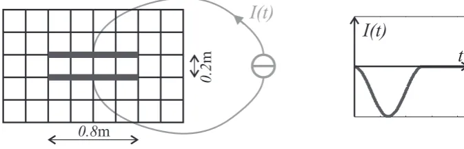
Fig. 2. Model problem: Charging process of a 2D plate capacitor, driven by a 750 kHz current pulse.

2.2.3 Eigensolutions of the Iteration Matrices

For the eigenvalues of these iteration matrices one can find the relations

Leapfrog: |λG,LF(1t )| =1 ⇔ 1t≤1t0 (20a)

ADI: |λG,ADI(1t )| =1 ∀1t >0, (20b)

which are a sufficient condition for the stability of the meth-ods. Whereas the LF method is restricted to time steps below the Courant limit1t≤1t0, the ADI method is

uncondition-ally stable for arbitrary time steps.

In most practical cases the dimension of the iteration ma-trices is too large to perform a further numerical analysis. For the small test example presented below, however, the matri-ces are of manageable size, and the results of Eq. (20b) can be visualized as shown in Fig. 1.

For the leapfrog method (left), most of the eigenvalues lay on the unit circle of the complex plane (the stability limit). However, since the time step chosen in this example slightly exceeds the Courant limit (1t = 1.021t0), some eigenval-ues have left the unit circle atλG= −1 and are placed on the

negative real axis. The eigenvalues withλG,LF < −1 will

cause a instable time integration. In the ADI case (Fig. 1, right) all eigenvalues are exactly on the unit circle for arbi-trary time steps (here:1t =31t0).

Note that for both methods there is a multiple eigenvalue λG = 1, referring to so-called static eigenmodes

(electro-magnetic fields with eigenfrequencyω=0), which will not be changed by the time stepping algorithm.

3 Transient Modal Expansion

In the following, the LF and ADI schemes are applied to a 2D (TE) model problem adapted from Garcia et al. (2002). It describes the transient charging process of a simple plate capacitor, driven by a 750 kHz current pulse (cf. Fig. 2).

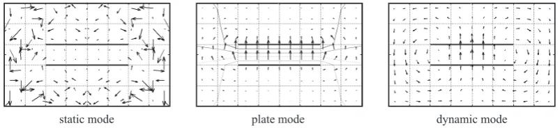
Figure 3 shows some eigenmodes of the related system matrix A: A static mode (left) with∇ ×E=0,λA =0 and

λG =1, a second static mode (’plate mode’) describing the

desired stationary field solution, and a dynamic mode (right) with∇ ×E6=0,λA6=0, andλG=eiϕ.

During the time stepping process the electric fields can now be decomposed into these (and all the other) eigen-modes. The results of this transient modal expansion, the expansion coefficients as a function of simulation time, are shown in Fig. 4 (Courant time step1t = 1t0) and Fig. 5 (enlarged time step1t =3·1t0).

static mode plate mode dynamic mode

Fig. 3. Model problem: Electric fields of a static eigenmode (gradient of a random discrete potential vector), the plate mode (stationary

solution of charging process), and a dynamic mode (oscillating eigenmode) in the plate capacitor.

t

Dt= t

D

plate mode (ADI/LF)

dynamic (ADI/LF)

static (ADI)

10

10

10

10

1

Fig. 4. Transient modal expansion coefficients (logarithmic scale)

for the Courant time step1t = 1t0: The leapfrog (LF) curves (which serve as a reference result) show the desired plate mode and some dynamic modes excited by the charging process, whereas all static modes are below round off. The ADI curves, however, include a parasitic static mode with a magnitude of about 10% of the total field at steady state.

the order of magnitude of the desired field solution (plate mode). This unphyiscal mode also qualitatively disturbes the stationary field solution, which is not shown here.

As the reason for this behaviour of ADI we postulate here the loss of orthogonality between the eigenvectors of the it-eration matrix: In the leapfrog scheme it can be easily shown that the electric part of the eigenvectors of the iteration ma-trix GLFand the system matrix A are identical, and that they

fulfill the same orthogonality condition Eq. (11). In the ADI scheme, however, this property is no longer valid: Although the static modes of GADIremain unchanged compared to the

static solutions of A (or GLF) — this can be proven for the

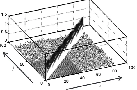
2D TE-case analyzed here — the dynamic modes now in-clude parts of the original static modes. As a consequence, energy can be transferred in each time step between these two classes of eigensolutions (which should be exactly sep-arated in continous theory). As a visualization of this fact, Fig. 6 shows the orthogonality pattern of the ADI-matrix for1t =3·1t0, exhibiting the parasitic coupling between static and dynamic solutions. As another consequence of this loss of consistency in the discrete model, the field solutions

10

10

10

10

1

D

t=3 t

D

static (ADI)

t

Fig. 5. Transient modal expansion coefficients (logarithmic scale)

for enlarged time step1t=3·1t0: The magnitude of the parasitic static mode in the ADI solution has considerably increased. No Leapfrog solutions are available abouve the Courant limit (instable time integration).

of ADI are no longer source-free, but parasitic electric and magnetic charges arise during the iteration. The intrinsic al-gebraic reason for these results is the splitting of the operator matrix C = C1+C2 in the derivation of the ADI-update equations. Since the spatial curl operator does no longer ap-pear as a whole in the update process, the consistency prop-erties Eqs. (5) and (6) are not applicable any more.

All these effects increase with a growing time step 1t. Although the ADI-method itself shows a 2nd order conver-gence for1t →0 (cf. also Garcia et al. (2002)), the results in this analysis show that the parasitic effect can be observed also for moderate time steps, even in the range of the Courant limit of the leapfrog method.

4 Conclusion

i j

Fig. 6. Orthogonality pattern

x_i,x_j

6=δij of the eigenmodes xi

of the ADI iteration matrix. The (degenerated) static modes can be orthogonalized, but the orthogonality between static and dynamic modes is lost. This unphysical effect increases with the time step width (here:1t=3·1t0).

does not conserve the energy of the original dynamic eigen-modes, even for moderate time steps. The main reason for this behaviour is the operator splitting in the construction of the ADI scheme, which leads to a loss of important con-sistency properties and of the orthogonality of the system’s eigensolutions. The same poor results also have to be ex-pected for similar schemes which are based on the idea of splitting the spatial operators to obtain unconditional stabil-ity of the time integration.

References

Darms, M.: Analyse des ADI Zeitintegrationsverfahrens f¨ur zeitlich ver¨anderliche Feldprobleme, Studienarbeit, Technische Univer-sit¨at Darmstadt, 2001.

Darms, M., Schuhmann, R., Spachmann, H., and Weiland, T.: Dispersion and Asymmetry Effects of ADI–FDTD, IEEE Mi-crowave and Wireless Components Letters, in press, 2003. Garcia, S. G., Lee, T., and Hagness, S. C.: On the Accuracy of the

ADI-FDTD Method, IEEE Antennas and Wireless Propagation Letters, 1, 31–34, 2002.

Kole, J. S., Figge M. T., and De Raedt, H.: Unconditionally Stable Algorithms to Solve the Time-Dependent Maxwell Equations, Physical Review E, 64, 066705, 2001.

Namiki, T.: 3-D ADI–FDTD Method – Unconditionally Stable Time-Domain Algorithm for Solving Full Vector Maxwell’s Equations, IEEE Trans. on Microwave Theory and Techniques, 48, 1743–1748, 2000.

Schuhmann, R. and Weiland, T.: Conservation of Discrete Energy and Related Laws in the Finite Integration Technique, Progress In Electromagnetics Research, PIER, 32, 301–316, 2001. Staker, S. and Piket-May, M.: Algorithm Study of ADI-FDTD,

Di-gest of the 2001 USNC/URSI National Radio Science Meeting, Boston, 255, 2001.

Weiland, T.: A Discretization Method for the Solution of Maxwell’s Equations for Six-Component Fields, Electronics and Communi-cation (AE ¨U), 31, 116, 1977a.

Weiland, T.: Time Domain Electromagnetic Field Computation with Finite Difference Methods, Int. Journal of Numerical Mod-elling, 9, 295–319, 1996.