MPGI International Conference 2014 (MPGIIC-2014 on 28th &29th March 2014) Published on: 29-03-2014
Ms. C.B. Tatepamulwar School of Computational Sciences,
S.R.T.M.University, Nanded. Email: [email protected]
QR Code for Mobile users
Face Recognition using Dynamic Inputs
Ms. C.B. Tatepamulwar, Dr. V. P. Pawar
School of Computational Sciences, S.R.T.M.University, Nanded.
ABSTRACT
Ideally a face detection system should be able to take a new face and return a name identifying that person. Mathematically, what possible approach would be robust and fairly computationally economical. If we have a database of people, every face has special features that define that person. One person may have a wider forehead, while another person has a scar on his right eyebrow from a rugby match as a young tuck. One technique may be to go through every person in the database and characterize it by these small features. Possible approach would be to take the face image as a whole identity. The goal of this paper is to extend the face recognition system to using dynamic inputs such as those obtained from CCTV cameras. This would involve detecting and tracking faces correctly in two or more cameras, pre-processing them and computing the disparity information prior to the identification stage.
ISSN: 2348-0351
Cite this article as:
Ms. C.B. Tatepamulwar, Dr. V. P. Pawar. Face Recognition using Dynamic Inputs. Asian Journal of Management Sciences.
13
1. Introduction
The human capacity to recognize particular individuals solely by observing the human face is quite remarkable. This capacity persists even through the passage of time, changes in appearance and partial occlusion. Because of this remarkable ability to generate near-perfect positive identifications, considerable attention has been paid to methods by which effective face recognition can be replicated on an electronic level. Certainly, if such a complicated process as the identification of a human individual based on a method as non-invasive as face recognition could be electronically achieved then fields such as bank and airport security could be vastly improved, identity theft could be further reduced and private sector security could be enhanced.
The eigenface technique finds a way to create ghost-like faces that represent the majority of variance in an image database. Our system takes advantage of these similarities between faces to create a fairly accurate and computationally "cheap" face recognition system[1]. Kirby and Sirovich pioneered the eigenface approach in 1988 at Brown University. Since then, many people have built and expanded on the basic ideas described in their original paper. We received the idea for our approach from a paper by Turk and Pentland based on similar research conducted at MIT.
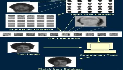
1. Eigen face system:
The eigenface face recognition system can be divided into two main segments: creation of the eigenface basis and recognition, or detection, of a new face. The system follows the following general flow:
Figure 1. A robust detection system can yield correct matches when the person is feeling happy or sad(source paper: 4.)
The idea of using eigenfaces was motivated by a technique for efficiently representing pictures of faces using Principal Component analysis(PCA). It is argued that a collection of face images can be approximately reconstructed by storing a small collection of weights for each face and a small set of standard pictures. Therefore, if a multitude of face images can be reconstructed by weighted sum of a small collection of characteristic images, then an efficient
way to learn and recognize faces might be to build the characteristic features from known face images and to recognize particular faces by comparing the feature weights needed to (approximately) reconstruct them with the weights associated with the known individuals.
The eigenfaces approach for face recognition involves the following initialization operations[1]:
1. Acquire a set of training images.
2. Calculate the eigenfaces from the training set, keeping only the best M images with the highest eigenvalues. These M images define the “face space”. As new faces are experienced, the eigenfaces can be updated. 3. Calculate the corresponding distribution in M
-dimensional weight space for each known individual (training image), by projecting their face images onto the face space.
Having initialized the system, the following steps are used to recognize new face images[1]:
1. Given an image to be recognized, calculate a set of weights of the M eigenfaces by projecting the it onto each of the eigenfaces.
2. Determine if the image is a face at all by checking to see if the image is sufficiently close to the face space. 3. If it is a face, classify the weight pattern as eigher a
known person or as unknown.
4. (Optional) Update the eigenfaces and/or weight patterns.
5. (Optional) Calculate the characteristic weight pattern of the new face image, and incorporate into the known faces.
1.1.Calculating Eigenfaces
Let a face image (x,y) be a two-dimensional N by N array of intensity values. An image may also be considered as a
vector of dimension
N
2, so that a typical image of size 256 by 256 becomes a vector of dimension 65,536, or equivalently, a point in 65,536-dimensional space. An ensemble of images, then, maps to a collection of points in this huge space[1,2,8,10].Images of faces, being similar in overall configuration, will not be randomly distributed in this huge image space and thus can be described by a relatively low dimensional subspace. The main idea of the principal component analysis is to find the vector that best account for the distribution of face images within the entire image space. These vectors define the subspace of face images, which
14 the original face images, and because they are face-like in appearance, they are referred to as “eigenfaces”.
Let the training set of face images be
1
,
2,
3, …, M.The average face of the set if defined by
M n n M 1 1 .Each face differs from the average by the vector
n n . Training set with the average face. Thisset of very large vectors is then subject to principal component analysis, which seeks a set of M orthonormal
vectors,
n, which best describes the distribution of thedata. The kth vector,
kis chosen such that
M n n T k k M 1 2 ) ( 1
... (1) is a maximum, subject to
otherwise k l k T l , 0 , 1
... (2)
The vectors
kand scalars
kare the eigenvectors andeigenvalues, respectively, of the covariance matrix
M n T T n n AA M C 1 1... (3)
where the matrix A[12...M]. The matrix C,
however, is
N
2 byN
2, and determining theN
2 eigenvectors and eigenvalues is an intractable task for typical image sizes. A computationally feasible method is needed to find these eigenvectors.If the number of data points in the image space is less
than the dimension of the space (
M
N
2), there will be onlyM
1
, rather thanN
2, meaningful eigenvectors (the remaining eigenvectors will have associatedeigenvalues of zero). Fortunately, we can solve for the
N
2 -dimensional eigenvectors in this case by first solving for the eigenvectors of and M by M matrix—e.g., solving a 16 x 16 matrix rather than a 16,384 x 16,384 matrix—and then taking appropriate linear combinations of the faceimages
n. Consider the eigenvectors
nof ATAsuchthat n n n T
A
A
... (4) Premultiplying both sides by A, we have
n n n T A A
AA
... (5)
from which we see that
A
nare the eigenvectors of TAA
C
.Following this analysis, we construct the M by M matrix
A A
L T , where n
T m mn
L
, and find the M
eigenvectors
nof L. These vectors determine linearcombinations of the M training set face images to form
the eigenfaces
n:M n A n M k k nk
n , 1,...,
1
... (6) With this analysis the calculations are greatly reduced,
from the order of the number of pixels in the images (
N
2) to the order of the number of images in the training set (M). In practice, the training set of face images will berelatively small (
M
N
2), and the calculations become quite manageable. The associated eigenvalues allow us to rank the eigenvectors according to their usefulness in characterizing the variation among the images.2. Principal component analysis:
PCA was invented in 1901 by Karl Pearson. PCA involves a mathematical procedure that transforms a number of possibly correlated variables into a number of uncorrelated variables called principal components, related to the original variables by an orthogonal transformation. This transformation is defined in such a way that the first principal component has as high a variance as possible (that is, accounts for as much of the variability in the data as possible), and each succeeding component in turn has the highest variance possible under the constraint that it be orthogonal to the preceding components. PCA is sensitive to the relative scaling of the original variables[1,3].
The major advantage of PCA is that the eigenface approach helps reducing the size of the database required for recognition of a test image. The trained images are not stored as raw images rather they are stored as their weights which are found out projecting each and every trained image to the set of eigenfaces obtained[5].
2.1.Eigenface Approach:
15 eigenvectors to obtain a set called eigenfaces. Every face has a contribution to the eigenfaces obtained. The best M eigenfaces from a M dimensional subspace is called “face space”. Each individual face can be represented exactly as the linear combination of “eigenfaces” or each face can also be approximated using those significant eigenfaces obtained using the most significant eigen values[6,7,8].
2.2.Steps to Calculate Eigenfaces:
1. Select the N images of size n X n from training database.
……….
Figure. 2 Images from local Database (Training Set)[Source paper:1] 2. Calculate the mean face image for the give set.
……….. (7 )
Figure. 3 Mean image of the local database (source paper: 1). 3. Calculate Zero mean image
Izi= Ii – Iavg where i≤0<N…………(8)
4. Convert all the images obtained in step 3 in one dimensional vector as shown in figure below, and get a matrix [Ø] where Øi is one dimensional form of Izi
---(9) Figure. 4 Concatenated Zero mean image matrix 5. Obtain a covariance matrix, zero mean matrix A as
A=[ Øt . Ø ] ………….(10) 6. Obtain Eigen value for covariance matrix [A]
Ax=λx and A-λIx ………..(11)
Solving this we get eigen values as
λ1 λ2 λ3 λ4 λ5……… λ1 ……….(12)
for each eigen value λi a associated eigen vector Xi is
present. Using this Xi with matrix [Ø] in equation 9 gives
Ø . Xi=Fi ………(13)
Convert each Fi into 2 dimensional images by reserving the
process of two dimension to one dimension.
7. Thus we get N eigenfaces Fi size nXn. Following figure
shows the eigenfaces for local database
Figure. 5 Sampled Eigenfaces local databases [source 1,9]
………(14) Reconstructed image is obtained as shown in figure below
Original Image Reconstructed Image
Figure. 6 Reconstruction face using eigenfaces[Source:10] The obtained eigenfaces are orthogonal to each other.
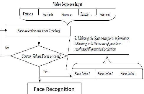
3. Video Based Face Recognition:
16 their method provides the infrastructure for recognizing face from video. Face tracking and pose estimation can be done by using their method. To a face recognition system by simply adding the view based eigenspace algorithm[4,9].
Figure 7. Scheme of Video based face recognition system(source: 9) It is thought to have been motivated by the way humans process faces for recognition and can easily be used with dynamic inputs such as CCTV images. Such images are small and are not suitable for use with most feature based methods. Appearance based methods like Eigenfaces are appropriate for such applications [8] and its use is in line with the long term goals of this work. We are proposed Scheme of Video based face recognition system.
4. Conclusion:
In this paper the face recognition based on PCA eigenfaces is studied for standard as well as locally created unconditional database. We present a comprehensive survey on video based face recognition. We have tried our best to provide researchers in the held with up-to-date information of research on video-based face recognition.
References:
1. Wikipedia,Workflow http://en.wikipedia.org/wiki/Workflow 2. http://marketing-cloud.com/
3. Lead Project, https://portal.leadproject.org/ 4. Wikipedia, ―Cyberinfrastructure,
http://en.wikipedia.org/wiki/Cyberinfrastructure 5. Nariman Mirzaei ―Cloud Computing
6. deborah collier ―Cloud Computing101:A brief introduction 7. Puja Dhar Cloud computing and its applications in the world of
networking
8. Amokrane, A. ; LIP6, UPMC-Univ. of Pierre & Marie 9. Curie, Paris, France ; Zhani, M.F. ; Langar, R. ; Boutaba,
10.R. ―Greenhead: Virtual Data Center Embedding across Distributed Infrastructures, IEEE Transactions on Cloud Computing, Volume:1 , Issue: 1 , Page36 – 49 ISSN 2168-7161 , September 2013
![Figure. 6 Reconstruction face using eigenfaces[Source:10]](https://thumb-us.123doks.com/thumbv2/123dok_us/8740556.1746037/4.612.326.568.137.688/figure-reconstruction-face-using-eigenfaces-source.webp)