Optimization of Optical Parametric Amplification
Efficiency in a Microresonator Under Ultrashort
Pump Wave Excitation
Ö züm Emre Aşırım*, Mustafa Kuzuoğlu
Department of Electrical and Electronics Engineering, Middle East Technical University, Ankara, Turkey
Abstract
This paper aims to computationally show that it is possible to achieve wideband high-gain optical parametricamplification in a very small low-loss microcavity. Our model involves numerical modeling of the charge polarization density in terms of the nonlinear electron cloud motion. Through a series of finite difference time domain simulations, we have determined the pump wave frequencies that maximize the electric energy density inside the microcavity. These pump wave frequencies that maximize the energy density are then selected for stimulus (input) wave amplification via nonlinear energy coupling. The achieved amplification factors are tabulated in terms of the pump wave frequency, stored electric energy density, and the intracavity charge polarization density. It is found that unlike what the current literature on nonlinear wave mixing suggests, micrometer-scale achievement of wideband high-gain optical parametric amplification is possible by choosing the optimum pump wave frequency that maximizes the stored electric energy density.
Keywords
Optical amplification, Nonlinear wave mixing, Optical microcavity, Parametric amplifier, Optimization1. Introduction
Electromagnetic wave amplification by nonlinear wave mixing has been studied extensively in the context of nonlinear optics [1]. It has been well established that we can amplify a relatively low power input wave, by using another wave of high intensity, which is called the pump wave, in a nonlinear medium [2]. The theory of electromagnetic wave amplification via nonlinear wave mixing involves the transfer of energy from the pump wave to the input wave as a result of nonlinear coupling in a medium that exhibits a strong nonlinear response under excitation [3]. The nonlinear wave mixing theory has been mostly investigated experimentally rather than computationally, especially for wave amplification purposes. The most important reason behind this trend is that, this concept is almost always studied in the micrometer or nanometer wavelength range, and yet the required medium length to observe any significant nonlinear effect is in the milimeter or centimeter range, which requires an extremely high computational cost for obtaining meaningful results, particularly for the purpose of wave amplification.
* Corresponding author:
[email protected] (Ö züm Emre Aşırım) Published online at http://journal.sapub.org/ijea
Copyright©2019The Author(s).PublishedbyScientific&AcademicPublishing This work is licensed under the Creative Commons Attribution International License (CC BY). http://creativecommons.org/licenses/by/4.0/
Furthermore, based on the current concept of wave amplification via nonlinear wave mixing a.k.a parametric
amplification, it is impossible to achieve a non-negligible
wave amplification in a few micron sized gain medium or a cavity. The required gain medium length for significant parametric amplification is mostly on the order of centimeters [4]. For this reason, the concept of parametric amplification is not feasible to be used for optical microsystems. In this paper, we have carried out a computational analysis that aims to show that it is possible to amplify a low power stimulus wave by mixing it with an intense pump wave of very short duration, in a wide range of frequencies and with a very large gain coefficient, inside a low-loss micro-cavity of several micrometers of length, by maximizing the stored pump wave energy in the cavity.
2. Intracavity Energy Density and the
Cavity Quality (Q) Factor
The Q factor is a measure of the energy storage capability of a cavity. A high Q value means that high energy can be stored in the cavity. It depends on the length of the cavity, the values of the reflection coefficients of the cavity walls, the frequency of the wave that is propagating inside the cavity, the total absorption coefficient of the medium between the cavity walls, and any kind of diffraction or scattering loss that can occur inside a cavity [14-16]. The Q factor of a cavity is defined as
𝐶𝐴𝑉𝐼𝑇𝑌 𝑄𝑈𝐴𝐿𝐼𝑇𝑌 𝑄 𝐹𝐴𝐶𝑇𝑂𝑅
= 2𝜋𝐸𝑛𝑒𝑟𝑔𝑦 𝑑𝑖𝑠𝑠𝑖𝑝𝑎𝑡𝑒𝑑 𝑝𝑒𝑟 𝑟𝑜𝑢𝑛𝑑 𝑡𝑟𝑖𝑝𝑆𝑡𝑜𝑟𝑒𝑑 𝑒𝑛𝑒𝑟𝑔𝑦 = 𝑓𝑇𝑟𝑡2𝜋𝜁 =4𝑓𝐿𝜋𝜁𝑐 . (1)
𝑇𝑟𝑡: 𝐶𝑎𝑣𝑖𝑡𝑦 𝑟𝑜𝑢𝑛𝑑 𝑡𝑟𝑖𝑝 𝑡𝑖𝑚𝑒
𝑓: 𝑊𝑎𝑣𝑒 𝑓𝑟𝑒𝑞𝑢𝑒𝑛𝑐𝑦
𝜁: 𝐹𝑟𝑎𝑐𝑡𝑖𝑜𝑛𝑎𝑙 𝑝𝑜𝑤𝑒𝑟 𝑙𝑜𝑠𝑠 𝑝𝑒𝑟 𝑟𝑜𝑢𝑛𝑑 𝑡𝑟𝑖𝑝 𝑐: 𝑆𝑝𝑒𝑒𝑑 𝑜𝑓 𝑙𝑖𝑔ℎ𝑡
𝐿: 𝐶𝑎𝑣𝑖𝑡𝑦 𝑙𝑒𝑛𝑔𝑡ℎ
The stored electric energy density in a medium depends on both the intensity of the electric field excitation, and the electric charge polarization density of the medium. Assuming a one dimensional analysis, the stored electric energy density in an isotropic medium is defined as [3]
𝑊𝑒 = 𝑆𝑡𝑜𝑟𝑒𝑑 𝑒𝑛𝑒𝑟𝑔𝑦 𝑑𝑒𝑛𝑠𝑖𝑡𝑦
=12𝐸𝐷 =12𝐸 𝜀∞𝐸 + 𝑃 =21𝜀∞𝐸2+12𝐸𝑃. (2)
𝐷: 𝐸𝑙𝑒𝑐𝑡𝑟𝑖𝑐 𝑓𝑙𝑢𝑥 𝑑𝑒𝑛𝑠𝑖𝑡𝑦
𝑃: 𝐸𝑙𝑒𝑐𝑡𝑟𝑖𝑐 𝑐ℎ𝑎𝑟𝑔𝑒 𝑝𝑜𝑙𝑎𝑟𝑖𝑧𝑎𝑡𝑖𝑜𝑛 𝑑𝑒𝑛𝑠𝑖𝑡𝑦 𝐸: 𝐸𝑙𝑒𝑐𝑡𝑟𝑖𝑐 𝑓𝑖𝑒𝑙𝑑 𝑖𝑛𝑡𝑒𝑛𝑠𝑖𝑡𝑦
𝜀∞: 𝐵𝑎𝑐𝑘𝑔𝑟𝑜𝑢𝑛𝑑 𝑖𝑛𝑓𝑖𝑛𝑖𝑡𝑒 𝑠𝑝𝑒𝑐𝑡𝑟𝑎𝑙 𝑏𝑎𝑛𝑑
𝑝𝑒𝑟𝑚𝑖𝑡𝑡𝑖𝑣𝑖𝑡𝑦
As an example case in which a very high energy can be stored inside a cavity, involves a dispersive medium, which has a frequency dependent permittivity as stated below [5]
𝜀 𝜔 = 1 + 𝜒 +𝑁𝑒𝑚𝜀2
0 1
𝜔2−𝜔02−𝑖𝛾𝜔 . (3)
𝑁: 𝐸𝑙𝑒𝑐𝑡𝑟𝑜𝑛 𝑑𝑒𝑛𝑠𝑖𝑡𝑦
𝜒: 𝐿𝑖𝑛𝑒𝑎𝑟 𝑒𝑙𝑒𝑐𝑡𝑟𝑖𝑐 𝑓𝑖𝑒𝑙𝑑 𝑠𝑢𝑠𝑐𝑒𝑝𝑡𝑖𝑏𝑖𝑙𝑖𝑡𝑦 𝛾: 𝑁𝑎𝑡𝑢𝑟𝑎𝑙 𝑑𝑎𝑚𝑝𝑖𝑛𝑔 𝑐𝑜𝑒𝑓𝑓𝑖𝑐𝑖𝑒𝑛𝑡 𝜔0: 𝐴𝑛𝑔𝑢𝑙𝑎𝑟 𝑟𝑒𝑠𝑜𝑛𝑎𝑛𝑐𝑒 𝑓𝑟𝑒𝑞𝑢𝑒𝑛𝑐𝑦
If 𝜔𝛾 ≪ (𝜔2− 𝜔02), then we can write [2]
𝜀 𝜔 = 1 + 𝜒 +𝑁𝑒𝑚𝜀2
0 1
𝜔2−𝜔02 . (4)
Assume that there are two monochromatic waves propagating inside a dispersive medium that is placed between two highly reflective walls, 𝑬𝟏 and 𝑬𝟐. Let us
assume that the angular frequency 𝜔 of 𝑬𝟏 is almost
equal to the resonance frequency of the medium (𝜔 ≈ 𝜔0),
then the stored energy in this cavity becomes extremely high. Now assume that 𝑬𝟐 has a significantly different
frequency than the resonance frequency of the medium. Unless it has a very high power, 𝑬𝟐 will not yield a
noticeable energy increase in the cavity as it’s frequency is not almost equal to the resonance frequency. Furthermore, 𝑬𝟐 will not be able to absorb any energy from the
energized cavity as there is no energy coupling mechanism, simply because the medium is linear. To account for an energy transfer from an energized cavity to a low power wave, we need a nonlinear wave propagation analysis between the cavity walls, and for nonlinearity to arise, either the medium itself must be highly nonlinear, or at least one of the waves that propagate inside the cavity must have a very high amplitude.
Figure 1. A cavity with a high electric energy density (due to 𝑬𝟏) and two propagating waves
3. Wave Propagation in Nonlinear Dispersive Media
Nonlinearity arises when at least one of the waves that propagate in a medium have a very high intensity. Such high intensities are only possible with very short duration pulses [6,8], such as the pulses of a mode locked laser, which have
𝑓0: 𝑅𝑒𝑠𝑜𝑛𝑎𝑛𝑐𝑒 𝑓𝑟𝑒𝑞𝑢𝑒𝑛𝑐𝑦 , 𝛾: 𝐷𝑎𝑚𝑝𝑖𝑛𝑔 𝑐𝑜𝑒𝑓𝑓𝑖𝑐𝑖𝑒𝑛𝑡
𝑳
𝑳′
𝑬𝟏 ( 𝝎 ≈ 𝝎𝟎 )
𝜞𝟏 𝜞𝟐
𝜀 ω ≈ 1 + 𝜒 +𝑁𝑒 2
𝑚𝜀0[ 1 𝜔2− 𝜔
02]
durations on the scale of picoseconds or femtoseconds [7,9,10]. When high intensity pulses have very short durations, which is almost always the case, we have to account for the wave dispersion, as the impulse response of the charge polarization density of many dielectric media last much longer in duration than the pulse durations of such high intensity pulses.
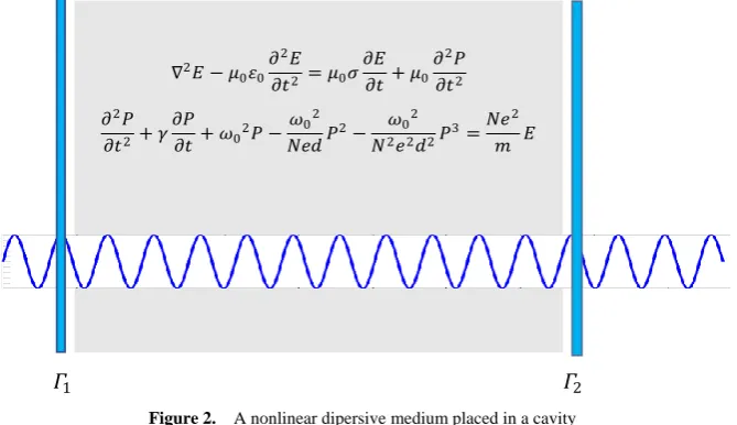
One can solve the wave equation in parallel with the nonlinear equation of motion of the electron cloud for a nonlinear dispersive medium. This is because the parameters such as the resonance frequency, damping coefficient, atom density, and atomic diameter have known values for most solids, which makes the simulation results much more meaningful and precise. In order to determine the time variation of the electric field in a nonlinear dispersive medium, we need to solve the following two equations [1]:
∇2𝐸 − 𝜇 0𝜀∞𝜕
2𝐸
𝜕𝑡2 = 𝜇0𝜎 𝜕𝐸 𝜕𝑡 + 𝜇0
𝜕2𝑃
𝜕𝑡2. (5) 𝜕2𝑃
𝜕𝑡2+ 𝛾 𝜕𝑃 𝜕𝑡 + 𝜔0
2𝑃 −𝜔02 𝑁𝑒𝑑𝑃
2− 𝜔02 𝑁2𝑒2𝑑2𝑃3=
𝑁𝑒2
𝑚 𝐸. (6)
𝑃: 𝐶ℎ𝑎𝑟𝑔𝑒 𝑝𝑜𝑙𝑎𝑟𝑖𝑧𝑎𝑡𝑖𝑜𝑛 𝑑𝑒𝑛𝑠𝑖𝑡𝑦 (𝐶𝑜𝑢𝑙𝑜𝑚𝑏/𝑚2), 𝑒: 𝐸𝑙𝑒𝑐𝑡𝑟𝑜𝑛 𝑐ℎ𝑎𝑟𝑔𝑒, 𝑚: 𝐸𝑙𝑒𝑐𝑡𝑟𝑜𝑛 𝑚𝑎𝑠𝑠
In Eq. (6) we have made an expansion up to the third order of the nonlinear charge polarization density as higher order terms will be negligibly small. For a dielectric medium, the electrical conductivity can be assumed as negligible (𝜎 ≈ 0). Some typical values for solid dielectric media are [1]
𝑅𝑒𝑠𝑜𝑛𝑎𝑛𝑐𝑒 𝑓𝑟𝑒𝑞𝑢𝑒𝑛𝑐𝑦: 𝑓0= 1.1 × 10¹⁵𝐻𝑧, 𝐷𝑎𝑚𝑝𝑖𝑛𝑔 𝑟𝑎𝑡𝑒: 𝛾 = 1 × 10⁹𝐻𝑧
𝐸𝑙𝑒𝑐𝑡𝑟𝑜𝑛 𝑑𝑒𝑛𝑠𝑖𝑡𝑦: 𝑁 = 3.5 × 1028/𝑚3, 𝐴𝑡𝑜𝑚𝑖𝑐 𝑑𝑖𝑎𝑚𝑒𝑡𝑒𝑟 ∶ 𝑑 = 0.3 𝑛𝑎𝑛𝑜𝑚𝑒𝑡𝑒𝑟𝑠
Figure 2. A nonlinear dipersive medium placed in a cavity
Consider the wave 𝐸2 that has a very high amplitude, without the presence of the low amplitude wave 𝐸1, the pair of
equations that describe the propagation of 𝐸2 in a nonlinear dispersive medium is given as
∇2 𝐸
2 − 𝜇0𝜀∞𝜕 2 𝐸2
𝜕𝑡2 = 𝜇0𝜎 𝜕 𝐸2
𝜕𝑡 + 𝜇0 𝜕2𝑃2
𝜕𝑡2. (7a) 𝜕2𝑃2
𝜕𝑡2 + 𝛾 𝜕𝑃2
𝜕𝑡 + 𝜔0 2 𝑃
2 −𝜔0 2
𝑁𝑒𝑑 𝑃2
2− 𝜔02
𝑁2𝑒2𝑑2 𝑃2 3=𝑁𝑒 2
𝑚 𝐸2 . (7b)
𝑃2: 𝐶ℎ𝑎𝑟𝑔𝑒 𝑝𝑜𝑙𝑎𝑟𝑖𝑧𝑎𝑡𝑖𝑜𝑛 𝑑𝑒𝑛𝑠𝑖𝑡𝑦 𝑑𝑢𝑒 𝑡𝑜 𝑡ℎ𝑒 𝑒𝑙𝑒𝑐𝑡𝑟𝑖𝑐 𝑓𝑖𝑒𝑙𝑑 𝐸2
𝑃1: 𝐶ℎ𝑎𝑟𝑔𝑒 𝑝𝑜𝑙𝑎𝑟𝑖𝑧𝑎𝑡𝑖𝑜𝑛 𝑑𝑒𝑛𝑠𝑖𝑡𝑦 𝑑𝑢𝑒 𝑡𝑜 𝑡ℎ𝑒 𝑒𝑙𝑒𝑐𝑡𝑟𝑖𝑐 𝑓𝑖𝑒𝑙𝑑 𝐸1
Now assume that 𝐸1 and 𝐸2 are propagating together in the same nonlinear dispersive medium, in this case the pair of
equations that represent the total electric field propagation is given as ∇2 𝐸
1+ 𝐸2 − 𝜇0𝜀∞𝜕 2 𝐸1+𝐸2
𝜕𝑡2 = 𝜇0𝜎 𝜕 𝐸1+𝐸2
𝜕𝑡 + 𝜇0 𝜕2 𝑃1+𝑃2
𝜕𝑡2 . (8a) 𝜕2(𝑃1+𝑃2)
𝜕𝑡2 + 𝛾 𝜕(𝑃1+𝑃2)
𝜕𝑡 + 𝜔0 2 𝑃
1+ 𝑃2 −𝜔0 2
𝑁𝑒𝑑 𝑃1+ 𝑃2
2− 𝜔02
𝑁2𝑒2𝑑2 𝑃1+ 𝑃2 3=𝑁𝑒 2
𝑚 𝐸1+ 𝐸2 . (8b)
We want to determine the propagation of the low amplitude wave 𝐸1 in the presence of the high amplitude wave 𝐸2, in
other words we want to determine the propagation of 𝐸1 when there is an energy coupling from 𝐸2 as a result of the
nonlinear interaction. In order to do that we subtract equations (7a,7b) from equations (8a,8b) respectively, which gives us ∇2 𝐸
1 − 𝜇0𝜀∞𝜕 2 𝐸1
𝜕𝑡2 = 𝜇0𝜎 𝜕 𝐸1
𝜕𝑡 + 𝜇0 𝜕2 𝑃1
𝜕𝑡2 . (9a) 𝜕2(𝑃1)
𝜕𝑡2 + 𝛾 𝜕(𝑃1)
𝜕𝑡 + 𝜔0 2 𝑃
1 −𝜔0 2 𝑁𝑒𝑑 𝑃1
2+ 2𝑃
1𝑃2 − 𝜔0 2 𝑁2𝑒2𝑑2{𝑃1
3+ 3𝑃
12𝑃2+ 3𝑃1𝑃22} =𝑁𝑒 2
𝑚 (𝐸1) (9b) ∇2𝐸 − 𝜇
0𝜀0
𝜕2𝐸
𝜕𝑡2 = 𝜇0𝜎
𝜕𝐸 𝜕𝑡+ 𝜇0
𝜕2𝑃
𝜕𝑡2
𝜕2𝑃
𝜕𝑡2 + 𝛾
𝜕𝑃
𝜕𝑡+ 𝜔02𝑃 − 𝜔02
𝑁𝑒𝑑𝑃2− 𝜔02
𝑁2𝑒2𝑑2𝑃3=
𝑁𝑒2 𝑚 𝐸
From equations {(7a,7b),(9a,9b)} we can see that 𝐸2 and 𝐸1 are coupled to each other. Based on equations (9a,9b), we
will investigate whether it is possible to amplify the low power electric field 𝐸1, by drawing energy from a low loss cavity
that is energized by the high power electric field 𝐸2.
Figure 3. Two waves are propagating through a nonlinear dipersive medium placed in a cavity
3.1. Finite Difference Time Domain Formulation of Energy Coupling in a Nonlinear Dispersive Medium
As introduced in the previous section, 𝐸2 is the high power wave that initiates the nonlinear energy coupling process
and 𝐸1 is the low power wave that will absorb energy from 𝐸2. The finite difference time domain formulation of this
process in a low-loss dispersive cavity requires the discretization of equations (7a,7b) and (9a,9b). Here we assume a one dimensional space along the x direction so that
∇2 𝐸 =𝜕2(𝐸)
𝜕𝑥2 (10)
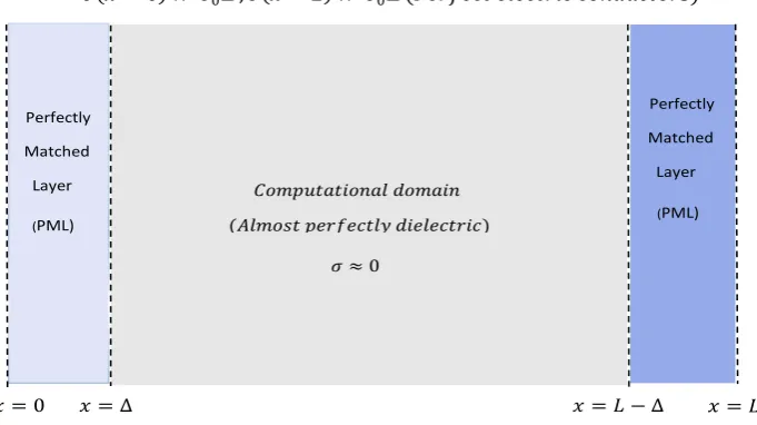
As in every computational problem that has an open (or reflectionless) boundary, we have to define a perfectly matched layer (PML) that must effectively surround and limit the computational region due to memory restrictions [17,18]. Since we are carrying out a one dimensional simulation, there is no issue of precise surrounding of the computational region by the PML. A PML is an artificial region and it surrounds the entire computational domain in order to absorb reflections [20,21]. By minimizing reflections, a PML allows us to obtain realistic results in a limited computational domain of a given problem. One method of realizing a PML is to define a conductivity gradient, by which we assign a zero conductivity at the computational domain interface of the PML, and we gradually increase the conductivity towards the outer PML boundary. Based on Fig. 4 the conductivity gradient that represents the PML region is defined as follows:
𝜎 𝑥 = 𝜎0 ∆ − 𝑥 , 0 < 𝑥 ≤ ∆
(𝑥 − (𝐿 − ∆))𝜎0 , (𝐿 − ∆) ≤ 𝑥 < 𝐿 (11a)
𝜎 𝑥 = 0 ≫ 𝜎0∆ , 𝜎 𝑥 = 𝐿 ≫ 𝜎0∆ (𝑃𝑒𝑟𝑓𝑒𝑐𝑡 𝑒𝑙𝑒𝑐𝑡𝑟𝑖𝑐 𝑐𝑜𝑛𝑑𝑢𝑐𝑡𝑜𝑟𝑠) (11b)
Figure 4. The domain of computation and the domain of termination (PML region)
𝑓0, 𝛾
𝜀𝑟
Nonlinear, dispersive material 𝑬𝟐
𝑬𝟏
𝛤1 𝛤2
𝐶𝑜𝑚𝑝𝑢𝑡𝑎𝑡𝑖𝑜𝑛𝑎𝑙 𝑑𝑜𝑚𝑎𝑖𝑛
(𝐴𝑙𝑚𝑜𝑠𝑡 𝑝𝑒𝑟𝑓𝑒𝑐𝑡𝑙𝑦 𝑑𝑖𝑒𝑙𝑒𝑐𝑡𝑟𝑖𝑐) (PML)
𝑥 = 𝐿 − ∆ 𝑥 = 𝐿
Perfectly
Matched
Layer Perfectly
Matched
Layer
(PML)
𝑥 = ∆ 𝑥 = 0
In order to match the intrinsic impedance of the PML region, to the intrinsic impedance of the computational region, we equate their permittivities and permeabilities at the junctions
𝜀∞ = 𝜀𝐶𝑜𝑚𝑝𝑢𝑡𝑎𝑡𝑖𝑜𝑛𝑎𝑙 = 𝜀𝑃𝑀𝐿 (12a)
µ0= µ𝐶𝑜𝑚𝑝𝑢𝑡𝑎𝑡𝑖𝑜𝑛𝑎𝑙 = µ𝑃𝑀𝐿 (12b)
lim𝑥→(𝐿−∆)−𝜀𝐶𝑜𝑚𝑝𝑢𝑡𝑎𝑡𝑖𝑜𝑛𝑎𝑙 = lim𝑥→(𝐿−∆)+𝜀𝑃𝑀𝐿 (13a) lim𝑥→(∆)−𝜀𝑃𝑀𝐿 = lim𝑥→(∆)+𝜀𝐶𝑜𝑚𝑝𝑢𝑡𝑎𝑡𝑖𝑜𝑛𝑎𝑙 (13b) lim𝑥→(𝐿−∆)−µ𝐶𝑜𝑚𝑝𝑢𝑡𝑎𝑡𝑖𝑜𝑛𝑎𝑙 = lim𝑥→(𝐿−∆)+µ𝑃𝑀𝐿 (13c) lim𝑥→(∆)−µ𝑃𝑀𝐿= lim𝑥→(∆)+µ𝐶𝑜𝑚𝑝𝑢𝑡𝑎𝑡𝑖𝑜𝑛𝑎𝑙 (13d)
Having the PML regions of our problem defined based on equations {(11a,11b),(12a,12b),(13a-13d)}, we can now discretize equations (7a,7b) and (9a,9b) using the finite difference time domain method. Let us first discretize equations (7a,7b) as follows:
𝐸2 𝑖 + 1, 𝑗 − 2𝐸2 𝑖, 𝑗 + 𝐸2 𝑖 − 1, 𝑗
∆𝑥2 − 𝜇0𝜀∞ 𝑖, 𝑗
𝐸2 𝑖, 𝑗 + 1 − 2𝐸2 𝑖, 𝑗 + 𝐸2 𝑖, 𝑗 − 1
∆𝑡2
= 𝜇0𝜎 𝑖, 𝑗 𝐸2 𝑖,𝑗 −𝐸∆𝑡2 𝑖,𝑗 −1 + 𝜇0𝑃2 𝑖,𝑗 +1 −2𝑃∆𝑡2 𝑖,𝑗 +𝑃2 2 𝑖,𝑗 −1 . (14)
𝑃2 𝑖, 𝑗 + 1 − 2𝑃2 𝑖, 𝑗 + 𝑃2 𝑖, 𝑗 − 1
∆𝑡2 + 𝛾
𝑃2 𝑖, 𝑗 − 𝑃2 𝑖, 𝑗 − 1
∆𝑡 + 𝜔02 𝑃2 𝑖, 𝑗
−𝜔02
𝑁𝑒𝑑 𝑃2 𝑖, 𝑗 2
− 𝜔02
𝑁2𝑒2𝑑2 𝑃2 𝑖, 𝑗 3
=𝑁𝑒𝑚2 𝐸2 𝑖, 𝑗 . (15)
Our aim is to solve for 𝐸2 𝑖, 𝑗 + 1 i.e. the value of 𝐸2 at a given point at the next time step. Since 𝐸2 is coupled to
𝑃2, we first solve for 𝑃2(𝑖, 𝑗 + 1) and then substitute it into the equation for 𝐸2 𝑖, 𝑗 + 1 . We keep on solving these two
equations iteratively for all time steps and for all points in the spatial domain of a given one dimensional problem. For a higher accuracy of the resulting solution, we choose ∆𝑡 and ∆𝑥 as small as possible [19,20].Now we discretize equations (9a,9b) and substitute the value of 𝑃2(𝑖, 𝑗) obtained from equations (7a,7b)
𝐸1 𝑖 + 1, 𝑗 − 2𝐸1 𝑖, 𝑗 + 𝐸1 𝑖 − 1, 𝑗
∆𝑥2 − 𝜇0𝜀∞ 𝑖, 𝑗
𝐸1 𝑖, 𝑗 + 1 − 2𝐸1 𝑖, 𝑗 + 𝐸1 𝑖, 𝑗 − 1
∆𝑡2
= 𝜇0𝜎 𝑖, 𝑗 𝐸1 𝑖,𝑗 −𝐸∆𝑡1 𝑖,𝑗 −1 + 𝜇0𝑃1 𝑖,𝑗 +1 −2𝑃∆𝑡1 𝑖,𝑗 +𝑃2 1 𝑖,𝑗 −1 . (16a)
𝑃1 𝑖, 𝑗 + 1 − 2𝑃1 𝑖, 𝑗 + 𝑃1 𝑖, 𝑗 − 1
∆𝑡2 + 𝛾
𝑃1 𝑖, 𝑗 − 𝑃1 𝑖, 𝑗 − 1
∆𝑡 + 𝜔02 𝑃1 𝑖, 𝑗 −
𝜔02
𝑁𝑒𝑑 𝑃1 𝑖, 𝑗
2
+ 2𝑃1 𝑖, 𝑗 𝑃2 𝑖, 𝑗
− 𝜔02
𝑁2𝑒2𝑑2{ 𝑃1 𝑖, 𝑗 3
+ 3 𝑃1 𝑖, 𝑗 2
𝑃2 𝑖, 𝑗 + 3𝑃1 𝑖, 𝑗 𝑃2 𝑖, 𝑗 2
} =𝑁𝑒𝑚2(𝐸1(𝑖, 𝑗)). (16b)
By solving these four equations simultaneously, along with the initial condition and the boundary conditions of a given problem, we can get the time variations of 𝐸1 and 𝐸2 at any point in one dimensional space. In order to test our
computational model, we have compared our computational results with the theoretical results in the well established context of nonlinear sum frequency generation in the appendix section. Now we move on to the simulation results.
4. Simulation Results
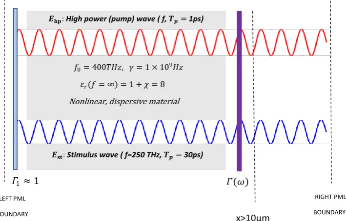
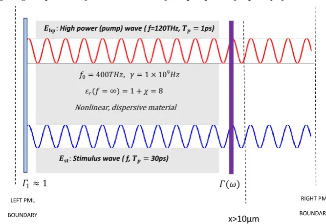
Simulation 1 - Part 1: Sweeping the pump wave frequency to maximize the intracavity energy density
Assume that a 250THz infrared stimulus wave 𝐸𝑠𝑡 and a high power pump wave 𝐸ℎ𝑝 (frequency to be determined) are
propagating inside a low-loss (high Q) cavity that has two reflecting walls. The reflecting wall on the left side can be thought as an optical isolator and has a reflection coefficient of 𝛤1≈ 1, the one on the right side represents a switch controlled optical
band-pass filter with a frequency dependent reflection coefficient 𝛤 𝑓 . Both waves are generated at x=0𝜇m and at the time instant t=0. The waves and the parameters of the gain medium are as given below:
𝐸ℎ𝑝(𝑥 = 0𝜇𝑚, 𝑡) = 2.25 × 10⁸× sin 2𝜋 𝑓𝑝𝑢𝑚𝑝 𝑡 𝑉/𝑚, 𝑓𝑜𝑟 0 ≤ 𝑡 ≤ 1𝑝𝑠 (𝑈𝑙𝑡𝑟𝑎𝑠ℎ𝑜𝑟𝑡 𝑝𝑢𝑙𝑠𝑒)
𝐸𝑠𝑡(𝑥 = 0𝜇𝑚, 𝑡) = 1 × sin 2𝜋 2.5 × 10¹⁴ 𝑡 𝑉/𝑚, 𝑓𝑜𝑟 0 ≤ 𝑡 ≤ 30𝑝𝑠
𝐷𝑖𝑒𝑙𝑒𝑐𝑡𝑟𝑖𝑐 𝑐𝑜𝑛𝑠𝑡𝑎𝑛𝑡 𝑜𝑓 𝑡ℎ𝑒 𝑔𝑎𝑖𝑛 𝑚𝑒𝑑𝑖𝑢𝑚 𝜀∞ = 8 (𝜇𝑟 = 1)
𝑅𝑒𝑠𝑜𝑛𝑎𝑛𝑐𝑒 𝑓𝑟𝑒𝑞𝑢𝑒𝑛𝑐𝑦 𝑜𝑓 𝑡ℎ𝑒 𝑔𝑎𝑖𝑛 𝑚𝑒𝑑𝑖𝑢𝑚 = 𝑓0= 400𝑇𝐻𝑧
𝐷𝑎𝑚𝑝𝑖𝑛𝑔 𝑐𝑜𝑒𝑓𝑓𝑖𝑐𝑖𝑒𝑛𝑡 𝑜𝑓 𝑡ℎ𝑒 𝑔𝑎𝑖𝑛 𝑚𝑒𝑑𝑖𝑢𝑚: 𝛾 = 1 × 10⁹𝐻𝑧
𝑆𝑝𝑎𝑡𝑖𝑎𝑙 𝑟𝑎𝑛𝑔𝑒 𝑜𝑓 𝑡ℎ𝑒 𝑔𝑎𝑖𝑛 𝑚𝑒𝑑𝑖𝑢𝑚: 0𝜇𝑚 < 𝑥 < 10𝜇𝑚
𝑅𝑖𝑔ℎ𝑡 𝑐𝑎𝑣𝑖𝑡𝑦 𝑤𝑎𝑙𝑙 𝑙𝑜𝑐𝑎𝑡𝑖𝑜𝑛: 𝑥 = 10µ𝑚; 𝐿𝑒𝑓𝑡 𝑐𝑎𝑣𝑖𝑡𝑦 𝑤𝑎𝑙𝑙 𝑙𝑜𝑐𝑎𝑡𝑖𝑜𝑛: 𝑥 = 0µ𝑚 𝐸𝑙𝑒𝑐𝑡𝑟𝑜𝑛 𝑑𝑒𝑛𝑠𝑖𝑡𝑦 𝑜𝑓 𝑡ℎ𝑒 𝑔𝑎𝑖𝑛 𝑚𝑒𝑑𝑖𝑢𝑚: 𝑁 = 3.5 × 1028/𝑚3
; 𝐴𝑡𝑜𝑚𝑖𝑐 𝑑𝑖𝑎𝑚𝑒𝑡𝑒𝑟 ∶ 𝑑 = 0.3 𝑛𝑚
Figure 5. Configuration of the cavity and the dielectric material specifications for simulation1-part1
During the whole simulation time, 𝛤 𝑓 = 1 for all 𝑓. The filter is used for post-processing of the results.
Our problem: Find the optimum pump wave frequency 𝑓𝑝𝑢𝑚𝑝 that maximizes 𝐸𝑠𝑡 in the cavity,
for 10THz < 𝑓𝑝𝑢𝑚𝑝 < 1000𝑇𝐻𝑧 (THz to UV), for 0𝜇𝑚 < 𝑥 < 10𝜇𝑚, 0 ≤ 𝑡 ≤ 30𝑝𝑠, such that
∇2 𝐸
ℎ𝑝 − 𝜇0𝜀∞ 𝜕2 𝐸ℎ𝑝
𝜕𝑡2 = 𝜇0𝜎 𝜕 𝐸ℎ𝑝
𝜕𝑡 + 𝜇0 𝜕2𝑃ℎ𝑝
𝜕𝑡2 . (7a) 𝜕2𝑃ℎ𝑝
𝜕𝑡2 + 𝛾 𝜕𝑃ℎ𝑝
𝜕𝑡 + 𝜔0 2 𝑃
ℎ𝑝 −𝜔0 2
𝑁𝑒𝑑 𝑃ℎ𝑝 2
− 𝜔02 𝑁2𝑒2𝑑2 𝑃ℎ𝑝
3
=𝑁𝑒𝑚2 𝐸ℎ𝑝 . (7b)
∇2 𝐸
𝑠𝑡 − 𝜇0𝜀∞𝜕 2 𝐸𝑠𝑡
𝜕𝑡2 = 𝜇0𝜎 𝜕 𝐸𝑠𝑡
𝜕𝑡 + 𝜇0 𝜕2 𝑃𝑠𝑡
𝜕𝑡2 . (9a)
𝜕2 𝑃 𝑠𝑡
𝜕𝑡2 + 𝛾
𝜕 𝑃𝑠𝑡
𝜕𝑡 + 𝜔02 𝑃𝑠𝑡 − 𝜔02
𝑁𝑒𝑑 𝑃𝑠𝑡2+ 2𝑃𝑠𝑡𝑃ℎ𝑝 − 𝜔02
𝑁2𝑒2𝑑2 𝑃𝑠𝑡3+ 3𝑃𝑠𝑡2𝑃ℎ𝑝+ 3𝑃𝑠𝑡𝑃ℎ𝑝2 = 𝑁𝑒2(𝐸𝑠𝑡)
𝑚 (9b) Initial conditions:
𝑃ℎ𝑝 𝑥, 0 = 𝑃ℎ𝑝′ 𝑥, 0 = 𝐸ℎ𝑝 𝑥, 0 = 𝐸ℎ𝑝′ 𝑥, 0 = 𝑃𝑠𝑡 𝑥, 0 = 𝑃𝑠𝑡′ 𝑥, 0 = 𝐸𝑠𝑡 𝑥, 0 = 𝐸𝑠𝑡′ 𝑥, 0 = 0
Boundary and excitation conditions:
𝐸ℎ𝑝(𝑥 = 0𝜇𝑚, 𝑡) = 2.25 × 10⁸× sin 2𝜋 𝑓𝑝𝑢𝑚𝑝 𝑡 𝑉/𝑚, 𝑓𝑜𝑟 0 ≤ 𝑡 ≤ 1𝑝𝑠 (𝑈𝑙𝑡𝑟𝑎𝑠ℎ𝑜𝑟𝑡 𝑝𝑢𝑙𝑠𝑒)
𝐸𝑠𝑡(𝑥 = 0𝜇𝑚, 𝑡) = 1 × sin 2𝜋 2.5 × 10¹⁴ 𝑡 𝑉/𝑚, 𝑓𝑜𝑟 0 ≤ 𝑡 ≤ 30𝑝𝑠
𝐸ℎ𝑝 𝑥 = 15𝜇𝑚, 𝑡 = 𝐸𝑠𝑡 𝑥 = 15𝜇𝑚, 𝑡 = 0 𝑓𝑜𝑟 0 < 𝑡 < 30𝑝𝑠 Absorbing boundary condition (perfectly matched layer):
𝜎 𝑥 = (𝑥 − (𝐿 − ∆))𝜎0 , (𝐿 − ∆) ≤ 𝑥 < 𝐿 , 𝑓𝑜𝑟 𝐿 = 15𝜇𝑚, ∆= 2.5𝜇𝑚, 𝜎0= 4.5 × 10⁸𝑆/𝑚
Optical isolator condition: Full reflection at x = 0μm
𝛤 𝑥 = 0𝜇𝑚, 𝑡 = 1 (𝑅𝑒𝑓𝑙𝑒𝑐𝑡𝑖𝑜𝑛 𝑐𝑜𝑒𝑓𝑓𝑖𝑐𝑖𝑒𝑛𝑡 𝑖𝑠 𝑒𝑞𝑢𝑎𝑙 𝑡𝑜 1)
Switch controlled optical bandpass filter condition: Full reflection at x = 10μm for t≤30 picoseconds, frequency dependent reflection at x = 10μm after t=30 picoseconds;
𝑓0= 400𝑇𝐻𝑧, 𝛾 = 1 × 10⁹𝐻𝑧
𝜀𝑟(𝑓 = ∞) = 1 + 𝜒 = 8
Nonlinear, dispersive material 𝑬𝐡𝐩: High power (pump) wave ( f, 𝑻𝒑= 1ps)
𝑬𝐬𝐭: Stimulus wave ( f=250 THz, 𝑻𝒑= 30ps)
𝛤1≈ 1 𝛤(𝜔)
LEFT PML
BOUNDARY
RIGHT PML
𝛤 𝑓′ =
1 𝑓𝑜𝑟 𝑎𝑙𝑙 𝑓′ , 𝑓𝑜𝑟 𝑥 = 10𝜇𝑚, 0 ≤ 𝑡 ≤ 30𝑝𝑠
1 − 𝑒−(
𝑓′−𝑓
2𝑇𝐻𝑧)2 , 𝑓𝑜𝑟 𝑥 = 10𝜇𝑚, 𝑡 > 30𝑝𝑠
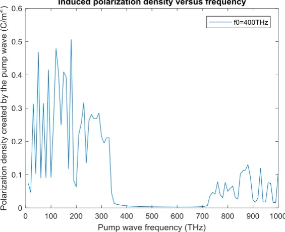
If amplified, the stimulus wave at t=30 picoseconds will not be monochromatic anymore, this will be due to the spectral broadening inside the cavity [11-13]. However, by adjusting the center frequency of the band-pass filter to be 250THz, we will get an amplified quasi-monochromatic output. The pump wave frequency will be varied from 10THz to 1000THz in 10THz increments and a pump wave frequency that yields a strong amplification of the stimulus wave will be chosen. The electric energy density 𝑊𝑒 and the charge polarization density 𝑃ℎ𝑝 created by the pump wave, are plotted with respect to
the pump wave frequency in Fig. 6 and Fig. 7 respectively. Stimulus wave amplitude gain versus pump wave frequency plot is shown in Fig. 8.
Figure 6. Maximum electric energy density created by the pump wave (for 0<t<30ps), as measured inside the cavity at x=5.73µm, versus the frequency of the pump wave
The maximum amplitude of the stimulus wave, versus pump wave frequency plot is shown in Fig. 8. Let us investigate the major amplification peak of the stimulus wave at 𝑓 = 120𝑇𝐻𝑧. The peak polarization density 𝑃ℎ𝑝 created by the pump
wave (which acts as the coupling coefficient), is high at this frequency. The peak electric energy density 𝑊𝑒created by the
pump wave is also high at 𝑓 = 120𝑇𝐻𝑧. Therefore we have an amplification peak at 𝑓 = 120𝑇𝐻𝑧. The same is true for all other peaks. If we have a look at Table 1, wherever the electric energy density and the polarization density created by the pump wave, are high, there is a stronger stimulus wave amplification.
Since the pump wave frequency of 𝑓 = 120𝑇𝐻𝑧 maximizes the intra-cavity energy and amplifies the stimulus wave, we choose this frequency as the frequency of pump wave excitation in order to compute the amplification (gain) spectrum of the stimulus wave. However, as already mentioned, the amplified stimulus wave is not monochromatic anymore due to the spectral broadening inside the cavity. Therefore, we must make a seperate analysis to obtain the gain spectrum of the stimulus wave, under a 120THz pump wave excitation.
𝑊𝑒: 𝑀𝑎𝑥𝑖𝑚𝑢𝑚 𝑒𝑙𝑒𝑐𝑡𝑟𝑖𝑐 𝑒𝑛𝑒𝑟𝑔𝑦 𝑑𝑒𝑛𝑠𝑖𝑡𝑦 𝑐𝑟𝑒𝑎𝑡𝑒𝑑 𝑏𝑦 𝑡ℎ𝑒 𝑝𝑢𝑚𝑝 𝑤𝑎𝑣𝑒 𝑖𝑛 𝑡ℎ𝑒 𝑐𝑎𝑣𝑖𝑡𝑦
𝑃ℎ𝑝: 𝑀𝑎𝑥𝑖𝑚𝑢𝑚 𝑐ℎ𝑎𝑟𝑔𝑒 𝑝𝑜𝑙𝑎𝑟𝑖𝑧𝑎𝑡𝑖𝑜𝑛 𝑑𝑒𝑛𝑠𝑖𝑡𝑦 𝑐𝑟𝑒𝑎𝑡𝑒𝑑 𝑏𝑦 𝑡ℎ𝑒 𝑝𝑢𝑚𝑝 𝑤𝑎𝑣𝑒 𝑖𝑛 𝑡ℎ𝑒 𝑐𝑎𝑣𝑖𝑡𝑦
𝐴𝑠𝑡,𝑚𝑎𝑥: 𝑀𝑎𝑥𝑖𝑚𝑢𝑚 𝑠𝑡𝑖𝑚𝑢𝑙𝑢𝑠 𝑤𝑎𝑣𝑒 𝑎𝑚𝑝𝑙𝑖𝑡𝑢𝑑𝑒 𝑖𝑛 𝑡ℎ𝑒 𝑐𝑎𝑣𝑖𝑡𝑦
Figure 8. Maximum stimulus wave amplitude between 0<t<30ps, as measured inside the cavity at x=5.73µm, versus the frequency of the pump wave
Table 1. Maximum stimulus wave amplitude (gain), maximum intracavity energy density created by the pump wave, maximum intracavity charge polarization density created by the pump wave, versus frequency of the pump wave. Gain maximizing pump wave frequency is indicated in bold
f(THz) 𝑊𝑒 𝑃ℎ𝑝 𝐴𝑠𝑡,𝑚𝑎𝑥 f(THz) 𝑊𝑒 𝑃ℎ𝑝 𝐴𝑠𝑡,𝑚𝑎𝑥
10 24587858 0.073549 29.68782 510 39410.43 0.00326 10.73229
20 10038549 0.046622 21.16144 520 37676.33 0.003208 10.72071
30 3.99E+08 0.312706 37.48459 530 37889.28 0.003121 10.76524
40 44698541 0.102643 8.542033 540 35060.39 0.003065 10.70476
50 5.32E+08 0.467588 1677835 550 36954.81 0.002982 10.92333
60 38094201 0.089774 53.50252 560 36226.29 0.002944 10.87302
70 4.92E+08 0.314052 82.48303 570 38002.19 0.00287 10.93508
80 38134542 0.090776 99.3708 580 35558.58 0.002833 10.90827
90 6.04E+08 0.414954 14730996 590 37412.51 0.002794 10.87437
100 34642254 0.091809 7.464663 600 36235.02 0.002764 10.92448
110 2.57E+08 0.257834 3414.097 610 35652.4 0.00273 11.09937
120 7.09E+08 0.478612 9.25E+08 620 36590.42 0.002712 11.07885
130 4.31E+08 0.405224 260720.9 630 37191.04 0.002706 11.1156
140 2.09E+08 0.249733 3352.826 640 38061.72 0.002724 11.1168
150 5.07E+08 0.408981 167951.1 650 39609.29 0.002772 11.23375
160 5.64E+08 0.393902 158069.7 660 41287.29 0.002839 11.31049
170 49943526 0.117305 7.338003 670 44207.1 0.002994 11.43198
180 5.53E+08 0.505682 436140.8 680 48415.29 0.003224 11.7344
190 21394526 0.082377 83.99106 690 54558.22 0.00357 11.83012
200 12609984 0.063049 20.24936 700 62270.26 0.00406 12.03565
210 1.38E+08 0.220572 62.19482 710 75584.37 0.004891 12.47808
220 1.89E+08 0.255036 279.9376 720 107466.8 0.007278 13.18134
230 2.12E+08 0.317012 880.1543 730 1009334 0.036879 21.99337
240 53238963 0.13555 25.35636 740 2078858 0.046548 33.81698
250 1.39E+08 0.260475 1114.391 750 2006865 0.041713 30.761
260 1.44E+08 0.281235 65709.25 760 9673896 0.078567 46.73325
270 1.76E+08 0.268166 3008.924 770 3255280 0.040102 243.0622
280 1.74E+08 0.267763 9804.008 780 2256265 0.030198 35.71366
290 1.78E+08 0.285167 61348.81 790 15803535 0.076385 100.6912
300 1.07E+08 0.214681 4015.914 800 7697947 0.049781 48.22146
310 62371087 0.194802 22.12135 810 13096084 0.059426 159.2424
320 56119926 0.210692 33.94152 820 18594988 0.06552 73.16598
330 57819494 0.210913 15.23713 830 4725648 0.030918 18.66814
340 2596324 0.044759 17.47628 840 4019403 0.026476 19.01043
350 348233.6 0.014213 11.1293 850 63409966 0.101802 55.50794
360 239292.5 0.010843 10.84791 860 80506507 0.111711 43.26424
370 179574.4 0.00915 10.6363 870 91022624 0.113907 67.34349
380 151083.5 0.008218 11.35786 880 1.27E+08 0.130152 63.39702
390 111890.1 0.00678 10.74123 890 69961073 0.092079 306.5119
400 105920.5 0.006284 10.80236 900 5394961 0.022793 27.93713
410 107563.3 0.005577 10.65824 910 3089991 0.017161 278.0156
420 70488.12 0.005131 10.63149 920 10570232 0.030793 192.1754
430 85887.48 0.004835 10.64494 930 1.32E+08 0.119193 1344.705
440 75463.67 0.004673 10.58697 940 3920668 0.01826 36.3059
450 59944.63 0.004191 10.55064 950 4451290 0.017481 19.01912
460 50390.5 0.003963 10.74716 960 66658661 0.075618 407.8365
470 48923.47 0.003791 10.61051 970 57676989 0.073767 1606.28
480 45454.85 0.003668 10.58697 980 4332888 0.015759 19.9839
490 43511.6 0.003503 10.68148 990 4195312 0.016605 31.25524
Part 2: Investigating the gain spectrum of the stimulus wave for a pump wave frequency of 120THz
Figure 10. The configuration for computing the gain spectrum of the stimulus wave for 𝑓𝑝𝑢𝑚𝑝 = 120𝑇𝐻𝑧
Our problem: Under an energy maximizing 120THz pump wave excitation, find the maximum stimulus wave amplitude (gain) 𝐸𝑠𝑡,𝑚𝑎𝑥 in the cavity for each stimulus wave frequency 𝑓𝑠𝑡𝑖𝑚𝑢𝑙𝑢𝑠, in the range 10THz < 𝑓𝑠𝑡𝑖𝑚𝑢𝑙𝑢𝑠 < 1000𝑇𝐻𝑧 (THz
to UV), for { 0𝜇𝑚 < 𝑥 < 10𝜇𝑚, 0 ≤ 𝑡 ≤ 30𝑝𝑠}, such that
∇2 𝐸
ℎ𝑝 − 𝜇0𝜀∞ 𝜕2 𝐸ℎ𝑝
𝜕𝑡2 = 𝜇0𝜎 𝜕 𝐸ℎ𝑝
𝜕𝑡 + 𝜇0 𝜕2𝑃ℎ𝑝
𝜕𝑡2 . (7a) 𝜕2𝑃ℎ𝑝
𝜕𝑡2 + 𝛾 𝜕𝑃ℎ𝑝
𝜕𝑡 + 𝜔0 2 𝑃
ℎ𝑝 −𝜔0 2 𝑁𝑒𝑑 𝑃ℎ𝑝
2
− 𝜔02 𝑁2𝑒2𝑑2 𝑃ℎ𝑝
3
=𝑁𝑒𝑚2 𝐸ℎ𝑝 . (7b)
∇2 𝐸
𝑠𝑡 − 𝜇0𝜀∞𝜕 2 𝐸𝑠𝑡
𝜕𝑡2 = 𝜇0𝜎 𝜕 𝐸𝑠𝑡
𝜕𝑡 + 𝜇0 𝜕2 𝑃𝑠𝑡
𝜕𝑡2 . (9a)
𝜕2 𝑃 𝑠𝑡
𝜕𝑡2 + 𝛾
𝜕 𝑃𝑠𝑡
𝜕𝑡 + 𝜔02 𝑃𝑠𝑡 −
𝜔02
𝑁𝑒𝑑 𝑃𝑠𝑡2+ 2𝑃𝑠𝑡𝑃ℎ𝑝
− 𝜔02
𝑁2𝑒2𝑑2 𝑃𝑠𝑡3+ 3𝑃𝑠𝑡2𝑃ℎ𝑝+ 3𝑃𝑠𝑡𝑃ℎ𝑝2 =𝑁𝑒 2(𝐸𝑠𝑡)
𝑚 (9b) Initial conditions:
𝑃ℎ𝑝 𝑥, 0 = 𝑃ℎ𝑝′ 𝑥, 0 = 𝐸ℎ𝑝 𝑥, 0 = 𝐸ℎ𝑝′ 𝑥, 0 = 𝑃𝑠𝑡 𝑥, 0 = 𝑃𝑠𝑡′ 𝑥, 0 = 𝐸𝑠𝑡 𝑥, 0 = 𝐸𝑠𝑡′ 𝑥, 0 = 0
Boundary conditions:
𝐸ℎ𝑝(𝑥 = 0𝜇𝑚, 𝑡) = 2.25 × 10⁸× sin 2𝜋 1.2 × 10¹⁴ 𝑡 𝑉/𝑚, 𝑓𝑜𝑟 0 ≤ 𝑡 ≤ 1𝑝𝑠, (120𝑇𝐻𝑧 )
𝐸𝑠𝑡(𝑥 = 0𝜇𝑚, 𝑡) = 1 × sin 2𝜋 𝑓𝑠𝑡𝑖𝑚𝑢𝑙𝑢𝑠 𝑡 𝑉/𝑚, 𝑓𝑜𝑟 0 ≤ 𝑡 ≤ 30𝑝𝑠
𝐸ℎ𝑝 𝑥 = 15𝜇𝑚, 𝑡 = 𝐸𝑠𝑡 𝑥 = 15𝜇𝑚, 𝑡 = 0 𝑓𝑜𝑟 0 < 𝑡 < 30𝑝𝑠 Absorbing boundary condition (perfectly matched layer):
𝜎 𝑥 = (𝑥 − (𝐿 − ∆))𝜎0 , (𝐿 − ∆) ≤ 𝑥 < 𝐿 , 𝑓𝑜𝑟 𝐿 = 15𝜇𝑚, ∆= 2.5𝜇𝑚, 𝜎0= 4.5 × 10⁸𝑆/𝑚
Optical isolator condition: Full reflection at x = 0μm
𝛤 𝑥 = 0𝜇𝑚, 𝑡 = 1 (𝑅𝑒𝑓𝑙𝑒𝑐𝑡𝑖𝑜𝑛 𝑐𝑜𝑒𝑓𝑓𝑖𝑐𝑖𝑒𝑛𝑡 𝑖𝑠 𝑒𝑞𝑢𝑎𝑙 𝑡𝑜 1)
Switch controlled optical bandpass filter condition: Full reflection at x = 10μm for t≤30 picoseconds, frequency dependent reflection at x = 10μm after t=30 picoseconds. For a given stimulus wave frequency ( f ), the magnitude frequency response of the filter is chosen to be
𝛤 𝑓′ =
1 𝑓𝑜𝑟 𝑎𝑙𝑙 𝑓′ , 𝑓𝑜𝑟 𝑥 = 10𝜇𝑚, 0 ≤ 𝑡 ≤ 30𝑝𝑠
1 − 𝑒−(
𝑓′−𝑓
2𝑇𝐻𝑧)2 , 𝑓𝑜𝑟 𝑥 = 10𝜇𝑚, 𝑡 > 30𝑝𝑠
𝑓0= 400𝑇𝐻𝑧, 𝛾 = 1 × 10⁹𝐻𝑧
𝜀𝑟(𝑓 = ∞) = 1 + 𝜒 = 8
Nonlinear, dispersive material
𝑬𝐡𝐩: High power (pump) wave ( f=120THz, 𝑻𝒑= 1ps)
𝑬𝐬𝐭: Stimulus wave ( f, 𝑻𝒑= 30ps)
𝛤1≈ 1 𝛤(𝜔)
LEFT PML
BOUNDARY
RIGHT PML
BOUNDARY
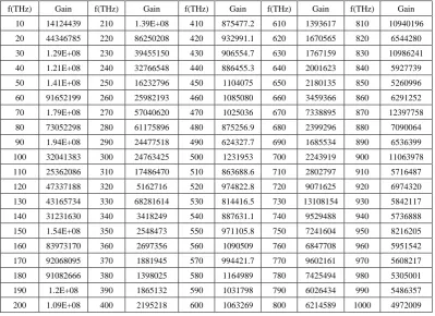
The amplification spectrum of the stimulus wave for 𝑓𝑝𝑢𝑚𝑝 = 120𝑇𝐻𝑧 is tabulated below in Table 2. The stimulus wave
is supplied to the cavity at t=0 as a quasi-monochromatic wave. For a given initial (at t=0) stimulus wave frequency, the center frequency of the band-pass filter is adjusted to be at the same frequency with the initial stimulus wave frequency. By doing so, we can observe how much gain can be obtained from the cavity for each initial stimulus wave frequency. We choose the pump wave frequency as 𝑓 = 120𝑇𝐻𝑧 as it maximizes the amplification, and we sweep the stimulus wave frequency from 10THz to 1000THz in 10THz increments.
Figure 11. Gain spectrum of the stimulus wave for 𝑓𝑝𝑢𝑚𝑝 = 120𝑇𝐻𝑧 and 𝑓0= 400𝑇𝐻𝑧
Table 2. Gain spectrum of the stimulus wave for 𝑓𝑝𝑢𝑚𝑝 = 120𝑇𝐻𝑧 and 𝑓0= 400𝑇𝐻𝑧
f(THz) Gain f(THz) Gain f(THz) Gain f(THz) Gain f(THz) Gain
10 14124439 210 1.39E+08 410 875477.2 610 1393617 810 10940196
20 44346785 220 86250208 420 932991.1 620 1670565 820 6544280
30 1.29E+08 230 39455150 430 906554.7 630 1767159 830 10986241
40 1.21E+08 240 32766548 440 886455.3 640 2001623 840 5927739
50 1.41E+08 250 16232796 450 1104075 650 2180135 850 5260996
60 91652199 260 25982193 460 1085080 660 3459366 860 6291252
70 1.79E+08 270 57040620 470 1025036 670 7338895 870 12397758
80 73052298 280 61175896 480 875256.9 680 2399296 880 7090064
90 1.94E+08 290 24477518 490 624327.7 690 1685534 890 6536399
100 32041383 300 24763425 500 1231953 700 2243919 900 11063978
110 25362086 310 17486470 510 863688.6 710 2802797 910 5716487
120 47337188 320 5162716 520 974822.8 720 9071625 920 6974320
130 43165734 330 68281614 530 814416.5 730 13108154 930 5842117
140 31231630 340 3418249 540 887631.1 740 9529488 940 5736888
150 1.54E+08 350 2548473 550 971105.8 750 7241604 950 8216205
160 83973170 360 2697356 560 1090509 760 6847708 960 5951542
170 92068095 370 1881945 570 994421.7 770 9602161 970 5608217
180 91082666 380 1398025 580 1164989 780 7425494 980 5305001
190 1.2E+08 390 1865132 590 1031798 790 6026434 990 5486357
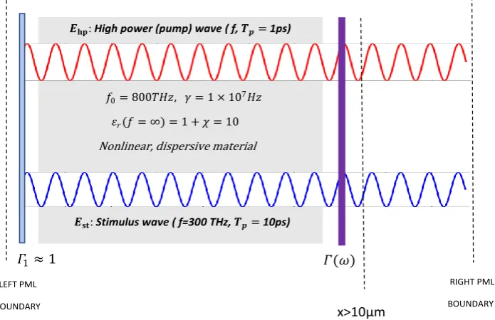
Simulation 2:
Part 1: Sweeping the pump wave frequency to maximize the intracavity energy density
Assume that a 300THz infrared stimulus wave 𝐸𝑠𝑡 and a high power pump wave 𝐸ℎ𝑝 (frequency to be determined) are
propagating inside a low-loss (high Q) cavity that has two reflecting walls. The reflecting wall on the left side can be thought as an optical isolator and has a reflection coefficient of 𝛤1≈ 1, the one on the right side represents a switch controlled optical
band-pass filter with a frequency dependent reflection coefficient 𝛤 𝑓 . Both waves are generated at x=0𝜇m and at the time instant t=0. The waves and the parameters of the gain medium are as given below:
𝐸ℎ𝑝(𝑥 = 0𝜇𝑚, 𝑡) = 5 × 10⁸× sin 2𝜋 𝑓𝑝𝑢𝑚𝑝 𝑡 𝑉/𝑚, 𝑓𝑜𝑟 0 ≤ 𝑡 ≤ 1𝑝𝑠 (𝑈𝑙𝑡𝑟𝑎𝑠ℎ𝑜𝑟𝑡 𝑝𝑢𝑙𝑠𝑒)
𝐸𝑠𝑡(𝑥 = 0𝜇𝑚, 𝑡) = 1 × sin 2𝜋 3 × 10¹⁴ 𝑡 𝑉/𝑚, 𝑓𝑜𝑟 0 ≤ 𝑡 ≤ 10𝑝𝑠
𝐷𝑖𝑒𝑙𝑒𝑐𝑡𝑟𝑖𝑐 𝑐𝑜𝑛𝑠𝑡𝑎𝑛𝑡 𝑜𝑓 𝑡ℎ𝑒 𝑔𝑎𝑖𝑛 𝑚𝑒𝑑𝑖𝑢𝑚 𝜀∞ = 10 (𝜇𝑟 = 1)
𝑅𝑒𝑠𝑜𝑛𝑎𝑛𝑐𝑒 𝑓𝑟𝑒𝑞𝑢𝑒𝑛𝑐𝑦 𝑜𝑓 𝑡ℎ𝑒 𝑔𝑎𝑖𝑛 𝑚𝑒𝑑𝑖𝑢𝑚 = 𝑓0= 800𝑇𝐻𝑧
𝐷𝑎𝑚𝑝𝑖𝑛𝑔 𝑐𝑜𝑒𝑓𝑓𝑖𝑐𝑖𝑒𝑛𝑡 𝑜𝑓 𝑡ℎ𝑒 𝑔𝑎𝑖𝑛 𝑚𝑒𝑑𝑖𝑢𝑚: 𝛾 = 1 × 10⁷𝐻𝑧
𝑇𝑖𝑚𝑒 𝑖𝑛𝑡𝑒𝑟𝑣𝑎𝑙 𝑎𝑛𝑑 𝑑𝑢𝑟𝑎𝑡𝑖𝑜𝑛 𝑜𝑓 𝑠𝑖𝑚𝑢𝑙𝑎𝑡𝑖𝑜𝑛: 0 ≤ 𝑡 ≤ 10𝑝𝑠 𝑆𝑝𝑎𝑡𝑖𝑎𝑙 𝑟𝑎𝑛𝑔𝑒 𝑜𝑓 𝑡ℎ𝑒 𝑔𝑎𝑖𝑛 𝑚𝑒𝑑𝑖𝑢𝑚: 0𝜇𝑚 < 𝑥 < 10𝜇𝑚
𝑅𝑖𝑔ℎ𝑡 𝑐𝑎𝑣𝑖𝑡𝑦 𝑤𝑎𝑙𝑙 𝑙𝑜𝑐𝑎𝑡𝑖𝑜𝑛: 𝑥 = 10µ𝑚; 𝐿𝑒𝑓𝑡 𝑐𝑎𝑣𝑖𝑡𝑦 𝑤𝑎𝑙𝑙 𝑙𝑜𝑐𝑎𝑡𝑖𝑜𝑛: 𝑥 = 0µ𝑚 𝐸𝑙𝑒𝑐𝑡𝑟𝑜𝑛 𝑑𝑒𝑛𝑠𝑖𝑡𝑦 𝑜𝑓 𝑡ℎ𝑒 𝑔𝑎𝑖𝑛 𝑚𝑒𝑑𝑖𝑢𝑚: 𝑁 = 3.5 × 1028/𝑚3
; 𝐴𝑡𝑜𝑚𝑖𝑐 𝑑𝑖𝑎𝑚𝑒𝑡𝑒𝑟 ∶ 𝑑 = 0.3 𝑛𝑚
Figure 12. Configuration of the cavity and the dielectric material specifications for simulation2-part1
During the whole simulation time, 𝛤 𝑓 = 1 for all 𝑓. The filter is used for post-processing of the results.
Our problem: Find the optimum pump wave frequency 𝑓𝑝𝑢𝑚𝑝 that maximizes 𝐸𝑠𝑡 in the cavity,
for 10THz < 𝑓𝑝𝑢𝑚𝑝 < 1000𝑇𝐻𝑧 (THz to UV), for 0𝜇𝑚 < 𝑥 < 10𝜇𝑚, 0 ≤ 𝑡 ≤ 10𝑝𝑠, such that
∇2 𝐸
ℎ𝑝 − 𝜇0𝜀∞ 𝜕2 𝐸ℎ𝑝
𝜕𝑡2 = 𝜇0𝜎 𝜕 𝐸ℎ𝑝
𝜕𝑡 + 𝜇0 𝜕2𝑃ℎ𝑝
𝜕𝑡2 . (7a) 𝜕2𝑃ℎ𝑝
𝜕𝑡2 + 𝛾 𝜕𝑃ℎ𝑝
𝜕𝑡 + 𝜔0 2 𝑃
ℎ𝑝 −𝜔0 2
𝑁𝑒𝑑 𝑃ℎ𝑝 2
− 𝜔02 𝑁2𝑒2𝑑2 𝑃ℎ𝑝
3
=𝑁𝑒𝑚2 𝐸ℎ𝑝 . (7b)
∇2 𝐸
𝑠𝑡 − 𝜇0𝜀∞𝜕 2 𝐸𝑠𝑡
𝜕𝑡2 = 𝜇0𝜎 𝜕 𝐸𝑠𝑡
𝜕𝑡 + 𝜇0 𝜕2 𝑃𝑠𝑡
𝜕𝑡2 . (9a)
𝜕2 𝑃 𝑠𝑡
𝜕𝑡2 + 𝛾
𝜕 𝑃𝑠𝑡
𝜕𝑡 + 𝜔02 𝑃𝑠𝑡 − 𝜔02
𝑁𝑒𝑑 𝑃𝑠𝑡2+ 2𝑃𝑠𝑡𝑃ℎ𝑝 − 𝜔02
𝑁2𝑒2𝑑2 𝑃𝑠𝑡3+ 3𝑃𝑠𝑡2𝑃ℎ𝑝+ 3𝑃𝑠𝑡𝑃ℎ𝑝2 = 𝑁𝑒2(𝐸𝑠𝑡)
𝑚 (9b)
𝑓0= 800𝑇𝐻𝑧, 𝛾 = 1 × 10⁷𝐻𝑧
𝜀𝑟(𝑓 = ∞) = 1 + 𝜒 = 10
Nonlinear, dispersive material 𝑬𝐡𝐩: High power (pump) wave ( f, 𝑻𝒑= 1ps)
𝑬𝐬𝐭: Stimulus wave ( f=300 THz, 𝑻𝒑= 10ps)
𝛤1≈ 1 𝛤(𝜔)
LEFT PML
BOUNDARY
RIGHT PML
Initial conditions:
𝑃ℎ𝑝 𝑥, 0 = 𝑃ℎ𝑝′ 𝑥, 0 = 𝐸ℎ𝑝 𝑥, 0 = 𝐸ℎ𝑝′ 𝑥, 0 = 𝑃𝑠𝑡 𝑥, 0 = 𝑃𝑠𝑡′ 𝑥, 0 = 𝐸𝑠𝑡 𝑥, 0 = 𝐸𝑠𝑡′ 𝑥, 0 = 0 Boundary and excitation conditions:
𝐸ℎ𝑝(𝑥 = 0𝜇𝑚, 𝑡) = 5 × 10⁸× sin 2𝜋 𝑓𝑝𝑢𝑚𝑝 𝑡 𝑉/𝑚, 𝑓𝑜𝑟 0 ≤ 𝑡 ≤ 1𝑝𝑠 (𝑈𝑙𝑡𝑟𝑎𝑠ℎ𝑜𝑟𝑡 𝑝𝑢𝑙𝑠𝑒)
𝐸𝑠𝑡(𝑥 = 0𝜇𝑚, 𝑡) = 1 × sin 2𝜋 3 × 10¹⁴ 𝑡 𝑉/𝑚, 𝑓𝑜𝑟 0 ≤ 𝑡 ≤ 10𝑝𝑠
𝐸ℎ𝑝 𝑥 = 15𝜇𝑚, 𝑡 = 𝐸𝑠𝑡 𝑥 = 15𝜇𝑚, 𝑡 = 0 𝑓𝑜𝑟 0 < 𝑡 < 10𝑝𝑠 Absorbing boundary condition (perfectly matched layer):
𝜎 𝑥 = (𝑥 − (𝐿 − ∆))𝜎0 , (𝐿 − ∆) ≤ 𝑥 < 𝐿 , 𝑓𝑜𝑟 𝐿 = 15𝜇𝑚, ∆= 2.5𝜇𝑚, 𝜎0= 4.5 × 10⁸𝑆/𝑚
Optical isolator condition: Full reflection at x = 0μm
𝛤 𝑥 = 0𝜇𝑚, 𝑡 = 1 (𝑅𝑒𝑓𝑙𝑒𝑐𝑡𝑖𝑜𝑛 𝑐𝑜𝑒𝑓𝑓𝑖𝑐𝑖𝑒𝑛𝑡 𝑖𝑠 𝑒𝑞𝑢𝑎𝑙 𝑡𝑜 1)
Switch controlled optical bandpass filter condition: Full reflection at x = 10μm for t≤10 picoseconds, frequency dependent reflection at x = 10μm after t=10 picoseconds;
𝛤 𝑓′ =
1 𝑓𝑜𝑟 𝑎𝑙𝑙 𝑓′ , 𝑓𝑜𝑟 𝑥 = 10𝜇𝑚, 0 ≤ 𝑡 ≤ 10𝑝𝑠
1 − 𝑒−(
𝑓′−𝑓
2𝑇𝐻𝑧)2 , 𝑓𝑜𝑟 𝑥 = 10𝜇𝑚, 𝑡 > 10𝑝𝑠
If amplified, the stimulus wave at t=10 picoseconds will not be monochromatic anymore, this will be due to the spectral broadening inside the cavity. However, by adjusting the center frequency of the band-pass filter to be 300THz, we will get an amplified quasi-monochromatic output. The pump wave frequency will be varied from 10THz to 1000THz in 10THz increments and a pump wave frequency that yields a strong amplification of the stimulus wave will be chosen. The electric energy density 𝑊𝑒 and the charge polarization density 𝑃ℎ𝑝created by the pump wave, are plotted with respect to the pump
wave frequency in Fig. 13 and Fig. 14 respectively. Stimulus wave amplitude gain versus pump wave frequency plot is shown in Fig. 15.
The maximum amplitude of the stimulus wave, versus pump wave frequency plot is shown in Fig. 15. Let us investigate the major amplification peak of the stimulus wave at 𝑓 = 350𝑇𝐻𝑧. The peak polarization density 𝑃ℎ𝑝 created by the pump
wave (which acts as the coupling coefficient), is high at this frequency. The peak electric energy density 𝑊𝑒created by the
pump wave is also high at 𝑓 = 350𝑇𝐻𝑧. Therefore we have an amplification peak at 𝑓 = 350𝑇𝐻𝑧. The same is true for all other peaks. If we have a look at Table 3, wherever the electric energy density and the polarization density created by the pump wave, are high, there is a stronger stimulus wave amplification.
Figure 14. Maximum charge polarization density created by the pump wave (for 0<t<10ps), as measured inside the cavity at x=5.73µm, versus the frequency of the pump wave
Figure 15. Maximum stimulus wave amplitude between 0<t<10ps, as measured inside the cavity at x=5.73µm, versus the frequency of the pump wave
Since the pump wave frequency of 𝑓 = 350𝑇𝐻𝑧 maximizes the intra-cavity energy and amplifies the stimulus wave, we choose this frequency as the frequency of pump wave excitation in order to compute the amplification (gain) spectrum of the stimulus wave. However, as already mentioned, the amplified stimulus wave is not monochromatic anymore due to the spectral broadening inside the cavity. Therefore, we must make a seperate analysis to obtain the gain spectrum of the stimulus wave, under a 350THz pump wave excitation.
𝑊𝑒: 𝑀𝑎𝑥𝑖𝑚𝑢𝑚 𝑒𝑙𝑒𝑐𝑡𝑟𝑖𝑐 𝑒𝑛𝑒𝑟𝑔𝑦 𝑑𝑒𝑛𝑠𝑖𝑡𝑦 𝑐𝑟𝑒𝑎𝑡𝑒𝑑 𝑏𝑦 𝑡ℎ𝑒 𝑝𝑢𝑚𝑝 𝑤𝑎𝑣𝑒 𝑖𝑛 𝑡ℎ𝑒 𝑐𝑎𝑣𝑖𝑡𝑦
𝑃ℎ𝑝: 𝑀𝑎𝑥𝑖𝑚𝑢𝑚 𝑐ℎ𝑎𝑟𝑔𝑒 𝑝𝑜𝑙𝑎𝑟𝑖𝑧𝑎𝑡𝑖𝑜𝑛 𝑑𝑒𝑛𝑠𝑖𝑡𝑦 𝑐𝑟𝑒𝑎𝑡𝑒𝑑 𝑏𝑦 𝑡ℎ𝑒 𝑝𝑢𝑚𝑝 𝑤𝑎𝑣𝑒 𝑖𝑛 𝑡ℎ𝑒 𝑐𝑎𝑣𝑖𝑡𝑦
Table 3. Maximum stimulus wave amplitude (gain), maximum intracavity energy density created by the pump wave, maximum intracavity charge polarization density created by the pump wave, versus frequency of the pump wave. Gain maximizing pump wave frequency is indicated in bold
f(THz) 𝐴𝑠𝑡,𝑚𝑎𝑥 𝑊𝑒 𝑃ℎ𝑝 f(THz) Gain We Php
10 5.883986 29699657 0.027091 510 1211.665 5.33E+08 0.200157
20 13.42542 5.13E+08 0.118397 520 12.03636 2.24E+08 0.128374
30 12.99005 48849682 0.033976 530 6380.668 6.2E+08 0.237481
40 9.096766 7.58E+08 0.14055 540 197.2572 4.04E+08 0.196768
50 17.10611 93371276 0.048789 550 2.228608 2E+08 0.118366
60 4.474521 6.09E+08 0.131476 560 3341.632 6.28E+08 0.211868
70 5.069646 1.42E+08 0.057396 570 50526.02 3.97E+08 0.160384
80 3.561172 2.05E+08 0.073801 580 1.952741 3.91E+08 0.160039
90 2.641755 74279614 0.042153 590 1.836473 1.45E+08 0.105914
100 4.077828 72125541 0.045394 600 2.067759 1.29E+08 0.103506
110 8.999627 6.04E+08 0.13448 610 2.159113 88756343 0.089169
120 2.613823 97309728 0.049051 620 7.876075 56936698 0.072166
130 3.933646 6.07E+08 0.135959 630 2.014397 1719389 0.012014
140 2.685399 89828810 0.047224 640 2.002486 867505.3 0.008003
150 2.446767 2.58E+08 0.08447 650 1.99723 594922.3 0.006319
160 2.277283 2.01E+08 0.071119 660 1.992377 454115.5 0.005502
170 2.568835 78977510 0.045889 670 1.992079 380584.9 0.004912
180 3.640279 7.35E+08 0.134221 680 1.99609 327444.1 0.004525
190 3.496944 50155368 0.036736 690 1.992056 281248.6 0.004147
200 5.209949 69704490 0.045108 700 1.994624 254086.5 0.003786
210 39.38512 1.25E+09 0.19136 710 2.003631 239090.8 0.003631
220 17.4777 9.3E+08 0.155742 720 2.008237 224470.1 0.003453
230 3.781144 73950854 0.046904 730 2.014686 212223.1 0.003299
240 6.847807 79718064 0.049873 740 2.08819 194997.7 0.00319
250 66.4612 1.03E+09 0.156807 750 2.020707 189412.7 0.003079
260 1354.073 3.03E+09 0.350968 760 2.026132 182209.2 0.003019
270 14.35446 4.2E+08 0.105385 770 2.031172 171364.8 0.002977
280 13.4472 65372520 0.045401 780 2.106717 167320.3 0.002944
290 6.311408 70860412 0.046055 790 2.062642 160819.4 0.002907
300 2.760757 83057212 0.048992 800 2.123964 154567 0.00289
310 2.27222 96378435 0.057127 810 2.074114 150234.4 0.002923
320 2.685882 1.17E+08 0.057266 820 2.043318 146722.7 0.002912
330 2.403513 60937048 0.046658 830 2.033978 142738.8 0.00291
340 1.907491 1.22E+08 0.06329 840 2.02517 137337.5 0.002947
350 6835947 2.2E+09 0.36398 850 2.07065 135352.4 0.002973
360 51.09379 5.4E+08 0.134201 860 2.042151 133736 0.003041
370 2.244881 82294755 0.055986 870 2.013683 130354.1 0.003091
380 4.045674 3.28E+08 0.099051 880 2.048405 129162.4 0.003179
390 2.385328 2.36E+08 0.099527 890 1.986717 133554.1 0.003284
400 1.914928 36407088 0.038589 900 2.000912 135280.2 0.003413
410 2.245768 1.57E+08 0.081641 910 1.981226 141468.3 0.003604
420 60.8144 1.04E+09 0.209959 920 2.02185 150727.1 0.003847
430 2.316941 1.14E+08 0.070736 930 2.017607 161806.4 0.004165
440 2.424293 74048560 0.059251 940 2.009308 175362.1 0.004584
450 1.903607 50132227 0.048627 950 2.004022 198713 0.005175
460 22.94166 4.85E+08 0.173972 960 2.00816 238825.9 0.006067
470 2.353593 2.17E+08 0.114367 970 2.008864 307733 0.008694
480 11.76979 3.42E+08 0.172466 980 122.4469 48819069 0.090452
490 7.203818 1.12E+08 0.097311 990 404.8945 1.14E+08 0.10242
Figure 16. Stimulus wave amplitude variation at x=5.73µm for a pump wave frequency of 350THz
Part 2: Investigating the gain spectrum of the stimulus wave for a pump wave frequency of 350THz
Figure 17. The configuration for computing the gain spectrum of the stimulus wave for 𝑓𝑝𝑢𝑚𝑝 = 350𝑇𝐻𝑧
Our problem: Under an energy maximizing 350THz pump wave excitation, find the maximum stimulus wave amplitude (gain) 𝐸𝑠𝑡,𝑚𝑎𝑥 in the cavity for each stimulus wave frequency 𝑓𝑠𝑡𝑖𝑚𝑢𝑙𝑢𝑠, in the range 10THz < 𝑓𝑠𝑡𝑖𝑚𝑢𝑙𝑢𝑠 < 1000𝑇𝐻𝑧 (THz
to UV), for { 0𝜇𝑚 < 𝑥 < 10𝜇𝑚, 0 ≤ 𝑡 ≤ 10𝑝𝑠}, such that ∇2 𝐸
ℎ𝑝 − 𝜇0𝜀∞ 𝜕2 𝐸ℎ𝑝
𝜕𝑡2 = 𝜇0𝜎 𝜕 𝐸ℎ𝑝
𝜕𝑡 + 𝜇0 𝜕2𝑃ℎ𝑝
𝜕𝑡2 . (7a) 𝜕2𝑃ℎ𝑝
𝜕𝑡2 + 𝛾 𝜕𝑃ℎ𝑝
𝜕𝑡 + 𝜔0 2 𝑃
ℎ𝑝 −𝜔0 2
𝑁𝑒𝑑 𝑃ℎ𝑝 2
− 𝜔02 𝑁2𝑒2𝑑2 𝑃ℎ𝑝
3
=𝑁𝑒𝑚2 𝐸ℎ𝑝 . (7b)
∇2 𝐸
𝑠𝑡 − 𝜇0𝜀∞𝜕 2 𝐸𝑠𝑡
𝜕𝑡2 = 𝜇0𝜎 𝜕 𝐸𝑠𝑡
𝜕𝑡 + 𝜇0 𝜕2 𝑃𝑠𝑡
𝜕𝑡2 . (9a)
𝜕2 𝑃 𝑠𝑡
𝜕𝑡2 + 𝛾
𝜕 𝑃𝑠𝑡
𝜕𝑡 + 𝜔02 𝑃𝑠𝑡 − 𝜔02
𝑁𝑒𝑑 𝑃𝑠𝑡
2+ 2𝑃 𝑠𝑡𝑃ℎ𝑝
− 𝜔02
𝑁2𝑒2𝑑2 𝑃𝑠𝑡3+ 3𝑃𝑠𝑡2𝑃ℎ𝑝+ 3𝑃𝑠𝑡𝑃ℎ𝑝2 = 𝑁𝑒2(𝐸𝑠𝑡)
𝑚 (9b)
𝑓0= 800𝑇𝐻𝑧, 𝛾 = 1 × 10⁷𝐻𝑧
𝜀𝑟(𝑓 = ∞) = 1 + 𝜒 = 10
Nonlinear, dispersive material
𝑬𝐡𝐩: High power (pump) wave ( f=350THz, 𝑻𝒑= 1ps)
𝑬𝐬𝐭: Stimulus wave ( f, 𝑻𝒑= 10ps)
𝛤1≈ 1 𝛤(𝜔)
LEFT PML
BOUNDARY
RIGHT PML
Initial conditions:
𝑃ℎ𝑝 𝑥, 0 = 𝑃ℎ𝑝′ 𝑥, 0 = 𝐸ℎ𝑝 𝑥, 0 = 𝐸ℎ𝑝′ 𝑥, 0 = 𝑃𝑠𝑡 𝑥, 0 = 𝑃𝑠𝑡′ 𝑥, 0 = 𝐸𝑠𝑡 𝑥, 0 = 𝐸𝑠𝑡′ 𝑥, 0 = 0 Boundary and excitation conditions:
𝐸ℎ𝑝(𝑥 = 0𝜇𝑚, 𝑡) = 5 × 10⁸× sin 2𝜋 3.5 × 10¹⁴ 𝑡 𝑉/𝑚, 𝑓𝑜𝑟 0 ≤ 𝑡 ≤ 1𝑝𝑠, (350𝑇𝐻𝑧 )
𝐸𝑠𝑡(𝑥 = 0𝜇𝑚, 𝑡) = 1 × sin 2𝜋 𝑓𝑠𝑡𝑖𝑚𝑢𝑙𝑢𝑠 𝑡 𝑉/𝑚, 𝑓𝑜𝑟 0 ≤ 𝑡 ≤ 10𝑝𝑠
𝐸ℎ𝑝 𝑥 = 15𝜇𝑚, 𝑡 = 𝐸𝑠𝑡 𝑥 = 15𝜇𝑚, 𝑡 = 0 𝑓𝑜𝑟 0 < 𝑡 < 10𝑝𝑠 Absorbing boundary condition (perfectly matched layer):
𝜎 𝑥 = (𝑥 − (𝐿 − ∆))𝜎0 , (𝐿 − ∆) ≤ 𝑥 < 𝐿 , 𝑓𝑜𝑟 𝐿 = 15𝜇𝑚, ∆= 2.5𝜇𝑚, 𝜎0= 4.5 × 10⁸𝑆/𝑚
Optical isolator condition: Full reflection at x = 0μm
𝛤 𝑥 = 0𝜇𝑚, 𝑡 = 1 (𝑅𝑒𝑓𝑙𝑒𝑐𝑡𝑖𝑜𝑛 𝑐𝑜𝑒𝑓𝑓𝑖𝑐𝑖𝑒𝑛𝑡 𝑖𝑠 𝑒𝑞𝑢𝑎𝑙 𝑡𝑜 1)
Switch controlled optical bandpass filter condition: Full reflection at x = 10μm for t≤10 picoseconds, frequency dependent reflection at x = 10μm after t=10 picoseconds. For a given stimulus wave frequency ( f ), the magnitude frequency response of the filter is chosen to be
𝛤 𝑓′ =
1 𝑓𝑜𝑟 𝑎𝑙𝑙 𝑓′ , 𝑓𝑜𝑟 𝑥 = 10𝜇𝑚, 0 ≤ 𝑡 ≤ 10𝑝𝑠
1 − 𝑒−(
𝑓′−𝑓
2𝑇𝐻𝑧)2 , 𝑓𝑜𝑟 𝑥 = 10𝜇𝑚, 𝑡 > 10𝑝𝑠
Table 4. Gain spectrum of the stimulus wave for 𝑓𝑝𝑢𝑚𝑝 = 350𝑇𝐻𝑧 and 𝑓0= 800𝑇𝐻𝑧
𝑓𝑠𝑡 (THz) Gain 𝑓𝑠𝑡(THz) Gain 𝑓𝑠𝑡(THz) Gain 𝑓𝑠𝑡(THz) Gain
10 155844.9 260 1501566 510 520598.5 760 39215.57
20 798352.4 270 269297.9 520 220764.7 770 15594.62
30 31826.07 280 39901.23 530 452107.7 780 38361.46
40 34628 290 77451.99 540 833534.4 790 16695.09
50 142339.1 300 167516 550 2134640 800 5713.115
60 94490.95 310 72228.5 560 1208588 810 7659.54
70 318353.9 320 288013 570 32903344 820 5866.713
80 282794.1 330 1451155 580 9814840 830 8579.433
90 57909.77 340 3397976 590 10268905 840 4303.018
100 224267.3 350 5710834 600 863060.1 850 6155.742
110 2894406 360 169142.8 610 636619.8 860 9586.705
120 150805.7 370 168433 620 226696.8 870 6767.037
130 117805.1 380 154531.2 630 59811.9 880 5462.442
140 60393.88 390 236854.6 640 13603.53 890 41621.51
150 35616.27 400 511870.7 650 61635.65 900 49452.8
160 21939.82 410 425733.8 660 27506.4 910 25727.11
170 17310.18 420 16540260 670 21122.59 920 269359.6
180 67314.37 430 18839603 680 33171.2 930 1753751
190 34687.58 440 9002002 690 14305.75 940 77485.81
200 28112.21 450 515299.4 700 6754.221 950 33980.92
210 153257.3 460 1223315 710 14424.94 960 60528.96
220 308297.8 470 293196.6 720 21193.08 970 83267.03
230 50972.36 480 72246.41 730 12675.06 980 393314.5
240 259557.2 490 40842.28 740 10614.65 990 590517.8
250 41309.18 500 143052.1 750 5628.318 1000 1808326
The amplification spectrum of the stimulus wave for 𝑓𝑝𝑢𝑚𝑝 = 350𝑇𝐻𝑧 is tabulated below in Table 4. The stimulus wave
doing so, we can observe how much gain can be obtained from the cavity for each stimulus wave frequency. We choose the pump wave frequency as 𝑓 = 350𝑇𝐻𝑧 as it maximizes the amplification, and we sweep the stimulus wave frequency from 10THz to 1000THz in 10THz increments.
Figure 18. Gain spectrum of the stimulus wave for 𝑓𝑝𝑢𝑚𝑝 = 350𝑇𝐻𝑧 and 𝑓0= 800𝑇𝐻𝑧
5. Conclusions
In order to amplify a low power stimulus wave via nonlinear wave mixing in a low-loss optical microcavity, a high intracavity energy is required. As a summary for intracavity energy maximization and efficient wave amplification, the following requirements should be met:
The cavity should have a high quality (Q) factor.
For a given resonance frequency (f0 ) of the material, the high power pump wave frequency fpump must be adjusted to
maximize the electric energy density inside the cavity.
Once these requirements are satisfied, it is possible to amplify a low power input wave, with a very large gain coefficient, by mixing it with an intense pump wave of very short duration, in a wide range of frequencies, inside a low-loss optical microcavity.
6. Appendix
6.1. Validation of the Computational Model and Results
In this section, we will compare our finite difference time domain based computational model with the theoretical formula in the well-established context of sum frequency generation via nonlinear wave mixing, in the following example.
Example: Nonlinear sum frequency generation (frequency upconversion)
This example is about the generation of a higher frequency component (𝜔3), by mixing of two monochromatic waves with
frequencies 𝜔1 and 𝜔2, such that 𝜔3= 𝜔2+ 𝜔1. In order to achieve this, at least one of the waves must have a high
intensity, so that nonlinearity arises, and wave mixing occurs.
The high amplitude pump wave 𝑬𝟐is generated at x=2.5𝜇m. Ithas an amplitude of 𝐴2V/m and a frequency of 180THz.
𝑬𝟐(𝑥 = 2.5𝜇𝑚, 𝑡) = 𝐴2× sin 2𝜋 1.8 × 10¹⁴ 𝑡 + 𝜑2 𝑉/𝑚
The input wave 𝑬𝟏is generated at x=2.5𝜇m. Ithas an amplitude of 𝐴1V/m and a frequency of 120THz.
𝑬𝟏(𝑥 = 2.5𝜇𝑚, 𝑡) = 𝐴1× sin 2𝜋 1.2 × 10¹⁴ 𝑡 + 𝜑1 𝑉/𝑚
𝐹𝑜𝑟 𝑠𝑖𝑚𝑝𝑙𝑖𝑐𝑖𝑡𝑦, 𝑎𝑠𝑠𝑢𝑚𝑒 𝑡ℎ𝑎𝑡 𝜑1= 0, 𝜑2= 0
Range of independent simulation variables: 0 ≤ 𝑥 ≤ 10𝜇𝑚, 0 ≤ 𝑡 ≤ 60𝑝𝑠
𝐷𝑎𝑚𝑝𝑖𝑛𝑔 𝑐𝑜𝑒𝑓𝑓𝑖𝑐𝑖𝑒𝑛𝑡 𝑜𝑓 𝑡ℎ𝑒 𝑖𝑛𝑡𝑒𝑟𝑎𝑐𝑡𝑖𝑜𝑛 𝑚𝑒𝑑𝑖𝑢𝑚: 𝛾 = 1 × 10¹²𝐻𝑧
𝐷𝑖𝑒𝑙𝑒𝑐𝑡𝑟𝑖𝑐 𝑐𝑜𝑛𝑠𝑡𝑎𝑛𝑡 𝑜𝑓 𝑡ℎ𝑒 𝑖𝑛𝑡𝑒𝑟𝑎𝑐𝑡𝑖𝑜𝑛 𝑚𝑒𝑑𝑖𝑢𝑚 𝜀∞ = 1 + 𝜒 = 10 (𝜇𝑟 = 1)
𝐿𝑒𝑓𝑡 𝑝𝑒𝑟𝑓𝑒𝑐𝑡𝑙𝑦 𝑚𝑎𝑡𝑐ℎ𝑒𝑑 𝑙𝑎𝑦𝑒𝑟 (𝑙𝑒𝑓𝑡 𝑎𝑏𝑠𝑜𝑟𝑝𝑡𝑖𝑜𝑛 𝑙𝑎𝑦𝑒𝑟) 𝑖𝑠 𝑓𝑟𝑜𝑚 𝑥 = 0 𝑡𝑜 𝑥 = 2.25𝜇𝑚 𝑅𝑖𝑔ℎ𝑡 𝑝𝑒𝑟𝑓𝑒𝑐𝑡𝑙𝑦 𝑚𝑎𝑡𝑐ℎ𝑒𝑑 𝑙𝑎𝑦𝑒𝑟 (𝑟𝑖𝑔ℎ𝑡 𝑎𝑏𝑠𝑜𝑟𝑝𝑡𝑖𝑜𝑛 𝑙𝑎𝑦𝑒𝑟) 𝑖𝑠 𝑓𝑟𝑜𝑚 𝑥 = 7.75𝜇𝑚 𝑡𝑜 𝑥 = 10𝜇𝑚
Figure 19. Configuration for frequency upconversion
The theoretical formula for frequency upconversion efficiency, which is derived from the solution of nonlinear wave equation that is based on material nonlinearity coefficient, is given as [1,4]
η𝑡ℎ𝑒𝑜𝑟𝑒𝑡𝑖𝑐𝑎𝑙 =𝜔𝜔3
2( sin 2𝑑 2𝑛3𝜔
32(𝑐𝑛𝜀0𝐴22)𝐿2 ) 2=𝜔𝜔3
2( sin 2𝑑 2𝑛4𝜔
32𝑐𝜀0𝐴22𝐿2 ) 2 (7)
𝜔2= 𝐹𝑟𝑒𝑞𝑢𝑒𝑛𝑐𝑦 𝑜𝑓 𝑡ℎ𝑒 𝑝𝑢𝑚𝑝 𝑤𝑎𝑣𝑒 , 𝜔1= 𝐹𝑟𝑒𝑞𝑢𝑒𝑛𝑐𝑦 𝑜𝑓 𝑡ℎ𝑒 𝑖𝑛𝑝𝑢𝑡 𝑤𝑎𝑣𝑒
d= Material nonlinearity coefficient, n= Refractive index
𝐴2= Pump wave amplitude, 𝐴1= Input wave amplitude, L= Length of the nonlinear media
𝜔3= 𝜔1+ 𝜔2= 𝐹𝑟𝑒𝑞𝑢𝑒𝑛𝑐𝑦 𝑜𝑓 𝑡ℎ𝑒 𝑢𝑝𝑐𝑜𝑛𝑣𝑒𝑟𝑡𝑒𝑑 𝑤𝑎𝑣𝑒
Our computational model is based on the finite difference time domain discretization of the nonlinear electron motion equation that involves the resonance frequency and the damping coefficient of the interaction medium. Coupled with the wave equation, the total wave 𝐸 = 𝐸1+ 𝐸2 can be evaluated from:
𝐸 𝑖+1,𝑗 −2𝐸 𝑖,𝑗 +𝐸 𝑖−1,𝑗
∆𝑥2 − 𝜇0𝜀∞ 𝑖, 𝑗
𝐸 𝑖,𝑗 +1 −2𝐸 𝑖,𝑗 +𝐸 𝑖,𝑗 −1
∆𝑡2 = 𝜇0𝜎 𝑖, 𝑗
𝐸 𝑖,𝑗 −𝐸 𝑖,𝑗 −1
∆𝑡 + 𝜇0
𝑃 𝑖,𝑗 +1 −2𝑃 𝑖,𝑗 +𝑃 𝑖,𝑗 −1 ∆𝑡2 . (8a) 𝑃 𝑖,𝑗 +1 −2𝑃 𝑖,𝑗 +𝑃 𝑖,𝑗 −1
∆𝑡2 + 𝛾
𝑃 𝑖,𝑗 −𝑃 𝑖,𝑗 −1
∆𝑡 + 𝜔0
2 𝑃 𝑖, 𝑗 −𝜔02
𝑁𝑒𝑑 𝑃 𝑖, 𝑗 2
− 𝜔02
𝑁2𝑒2𝑑2 𝑃 𝑖, 𝑗 3
=𝑁𝑒𝑚2 𝐸 𝑖, 𝑗 . (8b)
For a time interval of 0 ≤ 𝑡 ≤ 𝑡𝑚𝑎𝑥, the computational formula for frequency upconversion efficiency is
η𝑐𝑜𝑚𝑝𝑢𝑡𝑎𝑡𝑖𝑜𝑛𝑎𝑙 =Intensity of the 𝜔Intensity of the 𝜔3 frequency component of the total wave at t=𝑡𝑚𝑎𝑥
2 frequency component of the total wave at t=0 (9)
In this example, we have used the following values for each efficiency formula
𝜔2= 𝐹𝑟𝑒𝑞𝑢𝑒𝑛𝑐𝑦 𝑜𝑓 𝑡ℎ𝑒 𝑝𝑢𝑚𝑝 𝑤𝑎𝑣𝑒 = (2𝜋 × 180)𝑇𝐻𝑧 𝜔1= 𝐹𝑟𝑒𝑞𝑢𝑒𝑛𝑐𝑦 𝑜𝑓 𝑡ℎ𝑒 𝑖𝑛𝑝𝑢𝑡 𝑤𝑎𝑣𝑒 = (2𝜋 × 120)𝑇𝐻𝑧
L = Length of the nonlinear dispersive media=3.33 micrometers (from x=3.33𝜇𝑚 to 6.66𝜇𝑚) 𝜔3= 𝐹𝑟𝑒𝑞𝑢𝑒𝑛𝑐𝑦 𝑜𝑓 𝑡ℎ𝑒 𝑢𝑝𝑐𝑜𝑛𝑣𝑒𝑟𝑡𝑒𝑑 𝑤𝑎𝑣𝑒 = 2𝜋 × 300𝑇𝐻𝑧, n= 𝑅𝑒𝑓𝑟𝑎𝑐𝑡𝑖𝑣𝑒 𝑖𝑛𝑑𝑒𝑥 = 10
d = Material nonlinearity coefficient = 6.3 × 10⁻²² (The theoretical and the computational results agree for this value
of d for a sample pump wave amplitude of 𝐴2= 109𝑉/𝑚. Our aim is to see if the results also agree for all the other pump
wave amplitudes for this value of d)
𝐴2= Pump wave amplitude (varied from 5 × 10⁷𝑉/𝑚 𝑡𝑜 2 × 10⁹𝑉/𝑚 )
𝐴1= Input wave amplitude = 𝐴2/100 (𝐴1≪ 𝐴2)
𝑓0= 1100𝑇𝐻𝑧 𝛾 = 1 × 10¹²𝐻𝑧
𝜀𝑟(𝑓 = ∞) = 1 + 𝜒 = 10
Nonlinear, dispersive material 𝑬𝟐: ( f=180 THz, 𝑻𝒑= 60ps)
Figure 20. Comparison of the frequency upconversion efficiencies for 𝑓3=300THz and d= 6.3 × 10⁻²², versus the pump wave amplitude
REFERENCES
[1] Boyd Robert. W., Nonlinear Optics, Academic Press, New York, 2008.
[2] Fox Mark, Optical properties of solids, Oxford University Press, New York, 2002.
[3] Balanis Constantine. A., Advanced Engineering Electromagnetics, John Wiley & Sons, New York, 1989. [4] Bahaa E. A. Saleh, Malvin Carl Teich, Fundamentals of
Photonics, Wiley-Interscience, New York, 2007.
[5] Silfvast William.T., Laser Fundamentals, Cambridge University Press, New York, 2004.
[6] Junkichi Satsuma, Nobuo Yajima, “Initial Value Problems of One-Dimensional Self-Modulation of Nonlinear Waves in Dispersive Media”, Progress of Theoretical Physics Supplement, Volume 55, January 1974.
[7] Taflove Allen, Hagness Susan.C., Computational Electrodynamics: The Finite-Difference Time-Domain Method, Artech House, Boston, 2005.
[8] Amit S. Nagra, Robert A. York, “FDTD Analysis of Wave Propagation in Nonlinear Absorbing and Gain Media”, IEEE TRANSACTIONS ON ANTENNAS AND PROPAGATION, VOL. 46, NO. 3, MARCH 1998.
[9] Murray K. Reed, Michael K. Steiner-Shepard, Michael S. Armas, Daniel K. Negus, “Microjoule-energy ultrafast optical parametric amplifiers”, Journal of the Optical Society of America B, Volume 12, Issue 11, 1995.
[10] Anna G. Ciriolo, Matteo Negro, Michele Devetta, Eugenio Cinquanta, Davide Faccialà, Aditya Pusala, Sandro De Silvestri, Salvatore Stagira, and Caterina Vozzi, “Optical Parametric Amplification Techniques for the Generation of
High-Energy Few-Optical-Cycles IR Pulses for Strong Field Applications”, MDPI APPLIED SCIENCES, MARCH8 2017.
[11] E. A. Migal, F. V. Potemkin, and V. M. Gordienko, “Highly efficient optical parametric amplifier tunable from near-to mid-IR for driving extreme nonlinear optics in solids”, Optics Letters, Vol. 42, Issue 24, pp. 5218-5221, 2017.
[12] Chaohua Wu, Jingtao Fan, Gang Chen, and Suotang Jia, “Symmetry-breaking-induced dynamics in a nonlinear microresonator”, Opt. Express 27(20), 28133-28142 (2019). [13] Sung Bo Lee, Hyeon Sang Bark, and Tae-In Jeon, “Enhancement of THz resonance using a multilayer slab waveguide for a guided-mode resonance filter”, Opt. Express 27(20), 29357-29366 (2019).
[14] Houssein El Dirani, Laurene Youssef, Camille Petit-Etienne, Sebastien Kerdiles, Philippe Grosse, Christelle Monat, Erwine Pargon, and Corrado Sciancalepore, “Ultralow-loss tightly confining Si3N4 waveguides and high-Q microresonators”, Opt. Express, Vol. 27, Issue 21, pp. 30726-30740 (2019).
[15] Ivan S. Maksymov; Andrey A. Sukhorukov; Andrei V. Lavrinenko; Yuri S. Kivshar, “Comparative Study of FDTD-Adopted Numerical Algorithms for Kerr Nonlinearities”, IEEE Antennas and Wireless Propagation Letters, Year: 2011 | Volume: 10 | Journal Article | Publisher: IEEE.
[16] E. Valentinuzzi, “Dispersive properties of Kerr-like nonlinear optical structures”, Journal of Lightwave Technology, Year: 1998 | Volume: 16, Issue: 1 | Journal Article | Publisher: IEEE.
[17] Ozlem Ozgun, Mustafa Kuzuoglu, Metamaterials and Numerical Models, Nova Novinka; UK ed. Edition, 2011. [18] Ozlem Ozgun, Mustafa Kuzuoglu, MATLAB-based Finite
[19] Mohammad Amin Izadi, Rahman Nouroozi, “Adjustable Propagation Length Enhancement of the Surface Plasmon Polariton Wave via Phase Sensitive Optical Parametric Amplification”, Scientific Reports volume 8, Article number: 15495 (2018).
[20] Ozlem Ozgun, Mustafa Kuzuoglu, “Non-Maxwellian Locally-Conformal PML Absorbers for Finite Element Mesh
Truncation”, IEEE Transactions on Antennas and Propagation 55(3): 931 - 937 • April 2007.