Random Rotation Ensembles
Rico Blaser [email protected]
Piotr Fryzlewicz [email protected]
Department of Statistics London School of Economics Houghton Street
London, WC2A 2AE, UK
Editor:Charles Elkan
Abstract
In machine learning, ensemble methods combine the predictions of multiple base learners to construct more accurate aggregate predictions. Established supervised learning algo-rithms inject randomness into the construction of the individual base learners in an effort to promote diversity within the resulting ensembles. An undesirable side effect of this ap-proach is that it generally also reduces the accuracy of the base learners. In this paper, we introduce a method that is simple to implement yet general and effective in improv-ing ensemble diversity with only modest impact on the accuracy of the individual base learners. By randomly rotating the feature space prior to inducing the base learners, we achieve favorable aggregate predictions on standard data sets compared to state of the art ensemble methods, most notably for tree-based ensembles, which are particularly sensitive to rotation.
Keywords: feature rotation, ensemble diversity, smooth decision boundary
1. Introduction
Modern statistical learning algorithms combine the predictions of multiple base learners to form ensembles, which typically achieve better aggregate predictive performance than
the individual base learners (Rokach, 2010). This approach has proven to be effective
in practice and some ensemble methods rank among the most accurate general-purpose supervised learning algorithms currently available. For example, a large-scale empirical study (Caruana and Niculescu-Mizil, 2006) of supervised learning algorithms found that decision tree ensembles consistently outperformed traditional single-predictor models on a representative set of binary classification tasks. Data mining competitions also frequently feature ensemble learning algorithms among the top ranked competitors (Abbott, 2012).
some key examples. In bootstrap aggregation (Breiman, 1996), bootstrap replicates are used to construct multiple versions of a base predictor, which are subsequently aggregated via averaging or majority vote. This approach was found to be particularly effective for predictor classes that are unstable, in the sense that small variations of the input data lead to the construction of vastly different predictors (Hastie et al., 2009). Output smearing or flipping (Breiman, 2000) adds a different noise component to the dependent variable of each base predictor, which has a smoothing effect on the resulting decision boundary, leading to improved generalization performance. Boosting (Freund and Schapire, 1996) is an iterative procedure, where base learners are added sequentially in a forward stagewise fashion. By reweighting the data set at each iteration, later base learners are specialized to focus on the learning instances that proved the most challenging to the existing ensemble. In contrast to bootstrap aggregation, where each bootstrap sample is generated independently, boosting therefore does not lend itself naturally to parallel processing. Random decision forests (Ho, 1995, 1998) randomly select a feature subspace a priori and train a base learner in the chosen subspace using all available data. Instead of randomizing the training data, the structure of each predictor is altered by only including the chosen subset of predictors. Random forests (Breiman, 1999, 2001) combine bootstrap aggregation with the random projection method. At each tree node, a subset of the available predictors is randomly selected and the most favorable split point is found among these candidate predictors. This approach differs from random decision forests, where the selection of predictors is only performed once per tree. More generally, the framework also offers the possibility of using random linear combinations of two or more predictors. A summary of recent enhancements and applications of random forests can be found in Fawagreh et al. (2014). Perfect random tree ensembles (Cutler and Zhao, 2001), extremely random trees / extra trees (Geurts et al., 2006), and completely random decision trees (Liu et al., 2005; Fan et al., 2006) take ran-domization even further by not only selecting random predictor(s), as in random forests, but by also selecting a random split point, sometimes deterministically chosen from a small set of random candidate split points.
boosting projections (Garca-Pedrajas et al., 2007) provide a different, nonlinear view of the data to each base learner and oblique random forests (Menze et al., 2011) use linear discriminative models or ridge regression to select optimal oblique split directions at each tree node. Another approach that is related to but different from the method proposed in the present paper is embodied by rotation forests (Rodriguez et al., 2006; Kuncheva and Rodriguez, 2007), which take a subset of features and a bootstrap sample of the data and perform a principal component analysis (PCA), rotating the entire feature space before building the next base predictor. In addition to PCA, Kuncheva and Rodriguez (2007) experimented with nonparametric discriminate analysis (NDA) and sparse random projec-tions and in De Bock and Poel (2011), independent component analysis (ICA) is found to yield the best performance.
The premise of the present paper is that it makes sense to rotate the feature space in ensemble learning, particularly for decision tree ensembles, but that it is neither necessary nor desirable to do so in a structured way. This is because structured rotations reduce diversity. Instead, we propose to rotate the feature space randomly before constructing the individual base learners. The random rotation effectively generates a unique coordinate system for each base learner, which we show increases diversity in the ensemble without a significant loss in accuracy. In addition to rotation, affine transformations also include translation, scaling, and shearing (non-uniform scaling combined with rotation). However, only transformations involving rotation have an impact on base learners that are insensitive to monotone transformations of the input variables, such as decision trees. Furthermore, a key difference between random rotation and random projection is that rotations are re-versible, implying that there is no loss of information.
The remainder of this paper is structured as follows. Section 2 provides a motivational example for the use of random rotations using a well-known data set. In Section 3 we formally introduce random rotations and provide guidance as to their construction. Section 4 evaluates different application contexts for the technique and performs experiments to assesses its effectiveness. Conclusions and future research are discussed in Section 5. It is our premise that random rotations provide an intuitive, optional enhancement to a number of existing machine learning techniques. For this reason, we provide random rotation code in C/C++ and R in Appendix A, which can be used as a basis for enhancing existing software packages.
2. Motivation
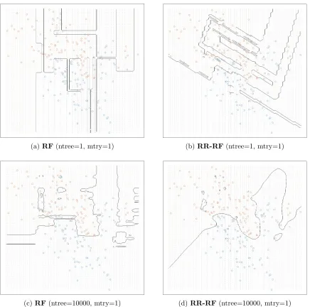
Figure 1 motivates the use of random rotations on the binary classification problem from chapter 2 of Hastie et al. (2009). The goal is to learn the decision boundary, which separates the two classes, from a set of training points. In this example, the training data for each class came from a mixture of ten low-variance Gaussian distributions, with individual means themselves distributed as Gaussian. Since the data is artificially generated, the optimal decision boundary is known by construction.
In this motivational example, we compare two approaches: (1) a standard random forest classifier and (2) a random forest classifier in which each tree is generated on a randomly
rotated feature space. It is evident that the random feature rotation has a significant
in the tree induction phase of the random forest algorithm – resulting in the same bootstrap samples and related feature subset selections at each decision branch for the two trees – the resulting tree is not merely a rotated version of the unrotated tree but is, in fact, a very different tree altogether, with a different orientation and a vastly different data partition. This demonstrates the power of the method; diversity is achieved with only a modest loss of information. However, the real benefit is illustrated on the bottom row of Figure 1 and arises from the aggregation of multiple randomly rotated trees. The rotated ensemble exhibits a visibly smoother decision boundary and one that is very close to optimal for this problem. The decision boundary is uncharacteristically smooth for a tree ensemble and is reminiscent of a kernel method, such as a k-nearest neighbor method or a support vector machine. In contrast, even with 10000 trees, the decision boundary for the standard random forest is still notably rectangular shaped. Another striking feature of the random rotation ensemble is the existence of a nearly straight diagonal piece of the decision boundary on the far left. This would be difficult to achieve with an axis-parallel base learner without rotation and it agrees well with the true decision boundary in this example.
3. Random Rotations
In this section, we formally introduce random rotations and describe two practical methods for their construction.
A (proper) rotation matrix R is a real-valuedn×northogonal square matrix with unit
determinant, that is
RT =R−1 and|R|= 1. (1)
Using the notation from Diaconis and Shahshahani (1987), the set of all such matrices
forms the special orthogonal group SO(n), a subgroup of the orthogonal group O(n) that
also includes so-called improper rotations involving reflections (with determinant−1). More
explicitly, matrices inSO(n) have determinant|R|= 1, whereas matrices inO(n) may have
determinant |R|=d, with d∈ {−1,1}. Unless otherwise stated, the notationO(n) always
refers to the orthogonal group in this paper and is not related to the Bachman-Landau asymptotic notation found in complexity theory.
In order to perform a random rotation, we uniformly sample over all feasible rotations. Randomly rotating each angle in spherical coordinates does not lead to a uniform
distri-bution across all rotations for n > 2, meaning that some rotations are more likely to be
generated than others. It is easiest to see this is in 3 dimensions: suppose we take a unit
sphere, denoting the longitude and latitude by the two angles λ ∈ [-π, π] and φ ∈ [-π/2,
π/2]. If we divide the surface of this sphere into regions by dividing the two angles into
equal sized intervals, then the regions closer to the equator (φ = 0) are larger than the
regions close to the poles (φ=±π/2). By selecting random angles, we are equally likely to
arrive in each region but due to the different sizes of these regions, points tend to cluster
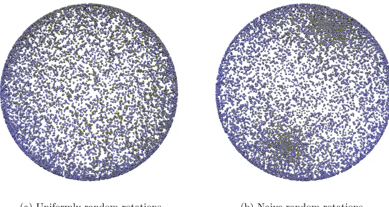
together at the poles. This is illustrated for n = 3 in Figure 2, where the undesirable
concentration of rotation points near the two poles is clearly visible for the naive method. In this illustration, the spheres are tilted to better visualize the areas near the poles.
The group O(n) does have a natural uniform distribution called the Haar measure,
which offers the distribution we need. Using the probabilistic notation from Diaconis and
(a)RF(ntree=1, mtry=1) (b)RR-RF(ntree=1, mtry=1)
(c)RF(ntree=10000, mtry=1) (d)RR-RF(ntree=10000, mtry=1)
(a) Uniformly random rotations (b) Naive random rotations
Figure 2: Comparison of correctly executed uniformly random rotation (left) in three di-mensions versus naive method of selecting two random angles in spherical coordi-nates (right). 10000 random rotations of the same starting vector were generated for each method and distances were computed between each pair of rotations to produce a rank-based gradient, with green dots representing those vectors with the lowest sums of distances.
P(R∈ΓU) for everyU ⊂O(n) and Γ∈O(n). Several algorithms exist to generate random
orthogonal matrices distributed according to the Haar measure overO(n), some of which are
documented in Anderson et al. (1987); Diaconis and Shahshahani (1987); Mezzadri (2007); Ledermann and Alexander (2011). We will focus on two basic approaches to illustrate the concept.
1. (Indirect Method) Starting with an n×nsquare matrix A, consisting ofn2 indepen-dent univariate standard normal random variates, a Householder QR decomposition
(Householder, 1958) is applied to obtain a factorization of the form A = QR, with
orthogonal matrix Qand upper triangular matrixR with positive diagonal elements.
The resulting matrix Q is orthogonal by construction and can be shown to be
uni-formly distributed. In other words, it necessarily belongs to O(n). Unfortunately,
if Q does not feature a positive determinant then it is not a proper rotation matrix
according to definition (1) above and hence does not belong to SO(n). However, if
this is the case then we can flip the sign on one of the (random) column vectors ofAto
obtainA+and then repeat the Householder decomposition. The resulting matrixQ+
is identical to the one obtained earlier but with a change in sign in the corresponding
column and|Q+|= 1, as required for a proper rotation matrix.
2. (Direct Method) A second method of obtaining random rotations involves selecting
accom-plished by drawingnindependent random normalN(0,1) variates{v1, v2, ..., vn} and
normalizing each by the square root of the sum of squares of all n variates, that is,
xi = vi/
p
v12+v22+. . .+v2
n for i∈ {1,2, . . . , n}. In other words, x is a unit vector
pointing to a random point on the n-sphere. This construction takes advantage of
spherical symmetry in the multivariate Normal distribution. The method is asymp-totically faster than the QR approach and an implementation is available in the GNU Scientific Library (Galassi, 2009) as function gsl ran dir nd. It should also be noted that it is straightforward to obtain the individual rotation angles from the random
vector x, which makes it possible to move from the (more compact) random vector
notation to the random rotation matrix used in the indirect method.
Generating random rotations in software for problems involving fewer than 1000 dimen-sions is straightforward and fast, even using the simple algorithm described above. Listings 2 and 3 in Appendix A provide examples of the indirect method in C++ and R respec-tively, both presented without error checking or optimizations. The C++ code takes less than 0.5 seconds on a single core of an Intel Xeon E5-2690 CPU to generate a 1000x1000 random rotation matrix. It uses the Eigen template library (Guennebaud et al., 2010) and a Mersenne Twister (Matsumoto and Nishimura, 1998) pseudorandom number generator. Larger rotation matrices can be computed with GPU assistance (Kerr et al., 2009) and may be pre-computed for use in multiple applications. In addition, for problems exceeding 1000 dimensions it is practical to only rotate a random subset of axes in order to reduce the computational overhead. We recommend that a different random subset is selected for each rotation in this case.
For categorical variables, rotation is unnecessary and ill defined. Intuitively, if a category is simply mapped to a new rotated category, there is no benefit in performing such a rotation.
4. Experiments
Random rotations complement standard learning techniques and are easily incorporated into existing algorithms. In order to examine the benefit of random rotations to ensemble performance, we modified three standard tree ensemble algorithms to incorporate random rotations before the tree induction phase. The necessary modifications are illustrated in pseudo code in Listing 1 below.
All methods tested use classification or regression trees that divide the predictor space
into disjoint regions Gj, where 1 ≤j ≤ J, with J denoting the total number of terminal
nodes of the tree. Extending the notation in Hastie et al. (2009), we represent a tree as
T(x;θ,Ω) =
J
X
j=1
cjI(R(x)∈Gj), (2)
with optimization parameters Ω = {Gj, cj}J1, random parameters θ = {R, ω}, where R is
the random rotation associated with the tree andω represents the random sample of (x, y)
pairs used for tree induction; I(·) is an indicator function. Each randomly rotated input
For regression,cj is typically just the average or median of all yj in region Gj. If we let |Gj|denote the cardinality ofGj, this can be written as
cj =
1
|Gj|
X
R(xk)∈Gj
yk. (3)
For classification trees, one of the modes is typically used instead.
Given a loss function L(yi, f(xi)), for example exponential loss for classification or
squared loss for regression, a tree-induction algorithm attempts to approximate the op-timization parameters for which the overall loss is minimized, that is
ˆ
Ω = arg min
Ω J
X
j=1 X
R(xi)∈Gj
L(yi, f(R(xi))) = arg min Ω
J
X
j=1 X
R(xi)∈Gj
L(yi, ci). (4)
This optimization is performed across all parameters Ω but the rotation is explicitly excluded
from the search space (R ∈ θ, but R 6∈ Ω) because we are advocating a random rotation
in this paper. However, conceptually it would be possible to include the rotation in the optimization in an attempt to focus on the most helpful rotations.
Listing 1: Testing Random Rotations (Pseudo Code)
I n p u t s : − t r a i n i n g f e a t u r e m a t r i x X − t e s t i n g f e a t u r e m a t r i x S − t o t a l number o f c l a s s i f i e r s M − s t a n d a r d b a s e l e a r n e r B
− a g g r e g a t i o n w e i g h t s w
(A) S c a l e o r rank numeric p r e d i c t o r s x ( S e c t . 4 . 2 ) : e . g . x0 := (x−Qk(x))/(Q1−k(x)−Qk(x))
(B) For m ∈ {1,2, . . . , M} do
( 1 ) g e n e r a t e random p a r a m e t e r s : θm:={Rm, ωm}
( 2 ) t r a i n s t a n d a r d l e a r n e r B on Rm(x) :
ˆ
Ωm= arg minΩP
J j=1
P
R(xi)∈GjL(yi, f(Rm(xi)))
( 3 ) compute t e s t o r out−o f−bag p r e d i c t i o n s T(x, θm,Ωm), x∈Rm(S)
(C) A g g r e g a t e p r e d i c t i o n s ( v o t e o r a v e r a g e ) fM(x) =P
M
m=1wmT(x;θm,Ωm)
The (regression) tree ensemble fM(x) can then be written as a weighted sum of the
individual trees, that is
fM(x) =
M
X
m=1
wmT(x;θm,Ωm), (5)
where M denotes the total number of trees in the ensemble. For classification ensembles,
a vote is typically taken instead. It should be noted that a separate rotation is associated with each tree in this notation but the same rotation could theoretically be associated with an entire group of trees. In particular, we can recover the standard setting without random
rotation by settingRm to the identity rotation for allm.
The difference between non-additive ensemble methods like random forests (Breiman, 2001) or extra trees (Geurts et al., 2006) and additive ensembles like boosted trees (Freund and Schapire, 1996) arises in the formulation of the joint model for multiple trees. As we will see, this difference makes testing random rotation with existing additive ensemble libraries much more difficult than with non-additive ensemble libraries. Specifically, random forests
and extra trees place an equal weight ofwm = 1/M on each tree, and trees are constructed
independently of each other, effectively producing an average ofM independent predictions:
ˆ
Ωm= arg min
Ωm
J
X
j=1 X
R(xi)∈Gj
L(yi, T(xi;θm,Ωm)). (6)
In contrast, boosted trees use wm = 1 and each new tree in the sequence is constructed to
reduce the residual error of the full existing ensemble fm−1(x), that is
ˆ
Ωm = arg min
Ωm
J
X
j=1 X
R(xi)∈Gj
L(yi, fm−1(xi) +T(xi;θm,Ωm)). (7)
There are other differences between the two approaches: for example,J, the number of leaf
nodes in each tree is often kept small for boosting methods in order to explicitly construct weak learners, while non-additive methods tend to use large, unpruned trees in an effort to reduce bias, since future trees are not able to assist in bias reduction in this case.
We mainly focus on random forest and extra tree ensembles in this paper because both of these algorithms rely on trees that are constructed independently of each other. This provides the advantage that the original tree induction algorithm can be utilized unmodified as a black box in the rotated ensemble, ensuring that any performance differences are purely due to the proposed random rotation and are not the result of any subtle differences (or dependencies) in the construction of the underlying trees.
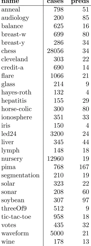
4.1 Data Sets & Preprocessing
Some algorithms tested were not able to handle categorical input variables or missing values and we performed the following automatic preprocessing steps for each data column:
1. Any column (predictors or response) with at least 10 distinct numeric values was treated as numeric and missing values were imputed using the column median.
2. Any column with fewer than 10 distinct values (numeric or otherwise) or with mostly non-numeric values was treated as categorical, and a separate category was explicitly created for missing values.
3. Categorical predictors with C categories were converted into (C −1) 0/1 dummy
variables, with the final dummy variable implied from the others to avoid adding multicollinearity.
Note that after evaluating these three rules, all predictors were either numeric without missing values or categorical dummy variables, with a separate category for missing values.
4.2 Variable Scaling
Rotation can be sensitive to scale in general and outliers in particular. In order to avoid biasing the results, we tested three different scaling methods, all of which only use in-sample information to calibrate the necessary parameters for out-of-sample scaling:
1. (Basic Scaling) Numeric values were scaled to [0,1] using the in-sample min and max values, that isx0= min(1,max(0,(x−min(xis))/(max(xis)−min(xis)))). This scaling
method deals with scale but only avoids out-of-sample outliers. Outliers are dealt with in a relatively crude fashion by applying a fixed cutoff.
2. (Quantile Scaling) Numeric values were linearly scaled in such a way that the 5th
and 95th percentile of the in-sample data map to 0 and 1 respectively, that is x0 =
(x−Q5(xis))/(Q95(xis)−Q5(xis)). In addition, any values that exceed these thresholds
were nonlinearly winsorized by adding/subtracting 0.01×log(1 + log(1 + ∆)), where
∆ is the absolute difference to the in-sample boundsQ5(xis) orQ95(xis). This robust
scaling has a breakdown point of 5% and maintains the order of inputs that exceed the thresholds.
3. (Relative Ranking) In-sample numeric valuesvi were augmented with{−∞,+∞}and
ranked as R(vi), such thatR(−∞) maps to 0 and R(+∞) maps to 1. Out-of-sample
data was ranked relative to this in-sample map. To accomplish this, the largest vi
is found that is smaller or equal to the out-of-sample data vo (call it vmaxi ) and the
smallest vi is found that is greater or equal to the out-of-sample data vo (vimin). The
4.3 Method & Evaluation
In order to collect quantitative evidence of the effect of random rotations, we built upon the
tree induction algorithms implemented in the widely used R packagesrandomForest (Liaw
and Wiener, 2002) andextraTrees (Simm and de Abril, 2013). For comparison, we also used
the following implementation of rotation forests: https://github.com/ajverster/RotationForest. Prior to the tests, all data sets were preprocessed and scaled using each of the three techniques described in the previous section (basic scaling, quantile scaling, and ranking).
Random forest and extra trees were tested with and without random rotation (for each scaling), while rotation forests included their own deterministic PCA rotation (Rodriguez et al., 2006) but were also run for each scaling method. Random rotations were tested with and without flip rotations. The combination of tree induction algorithms, scalings, and rotation options resulted in a total of 21 distinct experiments per data set.
For each experiment we performed a random 70-30 split of the data; 70% training data and the remaining 30% served as testing data. The split was performed uniformly at random but enforcing the constraint that at least one observation of each category level had to be present in the training data for categorical variables. This constraint was necessary to avoid situations, where the testing data contained category levels that were absent in the training set. Experiments were repeated 100 times (with different random splits) and the average performance was recorded.
In all cases we used default parameters for the tree induction algorithms, except that we built 5000 trees for each ensemble in the hope of achieving full convergence.
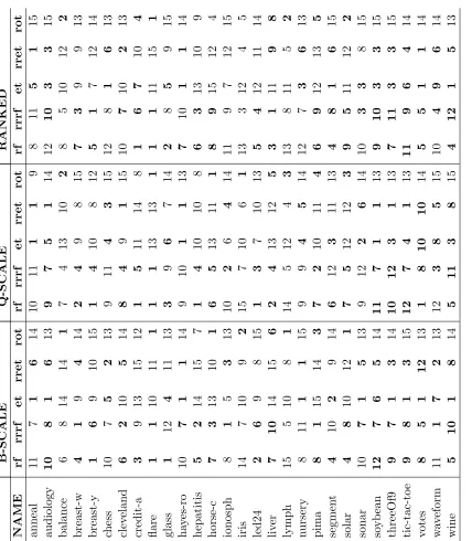
To evaluate the performance of random rotations, we ranked each method for each data set and computed the average rank across all data sets. This allowed us to compare performance of each method across scaling methods and tree induction algorithms in a consistent, nonparametric fashion. In addition, we determined the number of data sets for which each method performed within one cross-sectional standard deviation of the best predictor in order to obtain a measurement of significance. This approach is advocated in (Kuhn and Johnson, 2013) and it can be more informative when there is a cluster of strong predictors that is distinct from the weaker predictors and which would not get detected by simple ranking.
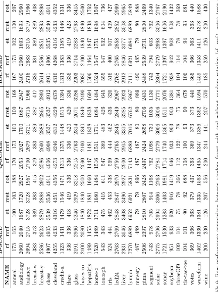
4.4 Results
In this table, we have omitted flip rotations because their performance was comparable to the simple random rotation, with flip rotations outperforming in 36% of cases, simple rotations outperforming in 45% of cases and ties in the remaining 19% of cases.
The best overall average rank of 6.10 (of 15) was achieved by the random rotation random forest algorithm with simple scaling, followed by the same algorithm with complex scaling (6.48) and ranking (6.55). This algorithm outperformed regardless of scaling. The next lowest rank of 6.72 was achieved by random rotation extra trees using quantile scaling. It is interesting to note that the average ranks for each scaling type were 7.50 for the complex scaling, 7.65 for the simple scaling and 7.81 for ranking. This indicates that the scaling method was less influential than the selection of the algorithm. In particular, the new method often improved on the original method even when only the ranks of the data were considered. We believe this to be an interesting result because it indicates that even rotating ranks can improve performance. Obviously, ranked data is completely robust to scaling effects and outliers.
The best average rank across scalings was achieved by random rotation random forests with 6.38, followed by extra trees (7.06), random forests (7.20), random rotation extra trees (7.26), and rotation forests (10.38).
In our tests, rotation forests underperformed overall but showed strong performance in some particular cases. The problem here was that when rotation forests did not excel at a problem, they often were the worst performer by a large margin, which had an impact on the average rank. In contrast, random rotation random forests rarely displayed the very best performance but often were among the top predictors. This insight led us to consider predictors that were within one cross-sectional standard deviation of the best predictor for each data set.
Random rotation random forests were within one standard deviation of the best result (highlighted in bold in Table 1) in 67.8% of cases, random forests without rotation in 64.3% of cases, extra trees (with and without rotation) in 49.4% of cases, and rotation forests in 27.6%. It appears to be clear that random rotation can improve performance for a variety of problems and should be included as a user option for standard machine learning packages. Random rotation appears to work best when numerical predictors outnumber categorical predictors, which are not rotated, and when these numerical predictors exhibit a relatively smooth distribution (rather than a few pronounced clusters). An example of a suitable dataset is Cleveland, with more than half of the variables continuous and spread out evenly. In contrast, Balance is an example of a dataset for which we cannot expect random rotation to perform well. However, in general it is difficult to judge the utility of rotation in advance and we recommend running a small test version of the problem with and without rotation to decide which to use: when the approach is successful, this tends to be apparent early.
Constructing a random rotation matrix using the indirect method described above
re-quires of the order ofp3 operations, wherepis the number of predictors to be rotated (time
complexity of QR factorization). Multiplying the resulting random rotation matrix with an
input vector requires of the order of p2 operations. During training, this step needs to be
performed k times, where k is the number of instances in the training data, for a total of
k×p2 operations. All but one of the UCI datasets contained fewer than 100 predictors,
seconds. However, as indicated above, for larger problems it does make sense to restrict the number of rotated predictors to maintain adequate performance.
Next, we consider the question of robustness.
4.5 Parameter Sensitivity and Extensions
In addition to the full tests described above, we also ran a few smaller examples to examine the sensitivity of random rotation to the choice of parameters in the underlying base learners.
For this, we used the well known UCI iris data set (4 numeric predictors, 3 classes, 150
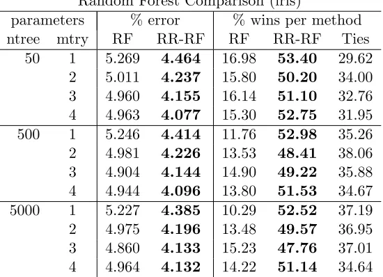
rows). Table 2 compares the performance of the standard random forest algorithm (RF) and a modified version including random feature rotation (RR-RF) on this data set.
Random Forest Comparison (iris)
parameters % error % wins per method
ntree mtry RF RR-RF RF RR-RF Ties
50 1 5.269 4.464 16.98 53.40 29.62
2 5.011 4.237 15.80 50.20 34.00
3 4.960 4.155 16.14 51.10 32.76
4 4.963 4.077 15.30 52.75 31.95
500 1 5.246 4.414 11.76 52.98 35.26
2 4.981 4.226 13.53 48.41 38.06
3 4.904 4.144 14.90 49.22 35.88
4 4.944 4.096 13.80 51.53 34.67
5000 1 5.227 4.385 10.29 52.52 37.19
2 4.975 4.196 13.48 49.57 36.95
3 4.860 4.133 15.23 47.76 37.01
4 4.964 4.132 14.22 51.14 34.64
Table 2: Performance comparison of the standard random forest algorithm (RF) and a mod-ified version with randomly rotated feature space for each tree (RR-RF) on the
iris data set. Ntree is the total number of trees in the forest, mtry the number of
randomly selected features considered at each decision node. Statistically signifi-cant differences in mean error percentage and win percentage at the 1% level are denoted in bold.
As in the detailed tests, both classifiers made use of the same tree induction algorithm,
implemented in the randomForest R package, but the feature space was randomly rotated
completed, a Wilcoxon signed-rank test was performed to compare the classification error percentage and win percentage of the original method with that of the modified classifier and to ascertain statistical significance at the 1% level. The modified ensemble featuring random rotation appears to universally outperform the original classifiers on this data set, regardless of parameter settings and in a statistically significant manner. However, it should be noted that the goal of this experiment was not to demonstrate the general usefulness of random rotations – this is achieved by the detailed experiments in the previous section – but rather to show the robustness to parameter changes for a specific data set.
Table 3 shows the analogous results for extra trees, which select both the split feature and the split point at random. Here we used the tree induction algorithm implemented in the extraTrees R package. In theory, there exist an infinite number of feasible split points (ncut) that could be chosen but for simplicity, we have only attempted ncut values in the range 1-4, meaning that at most 4 random split points were considered in the tests. The improvement due to rotation is again universal and statistically significant. For reasonable
parameters (e.g. ntree≥50), the new method matches or outperforms the original method
in over 94% of the randomly generated cases and the performance improvement is 21.7% on average. This is again a very encouraging result, as it demonstrates that the results above are robust, even if non-default parameters are used for the base learners. It is also interesting to note that randomly rotated extra tree ensembles outperform randomly rotated random forests here and they tend to do best with lower ncut values, indicating that more randomness (via rotation, feature selection, and split selection) is helpful for this particular problem.
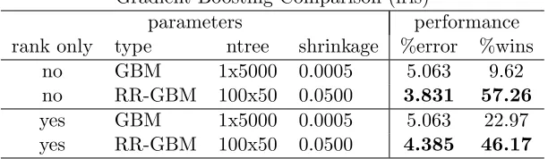
Table 4 shows comparable results with a gradient boosting machine from thegbm R package
(Ridgeway, 2013). Since boosting is an additive procedure, where later trees have an explicit dependence on earlier trees in the ensemble, the comparison of the two methods is not as straightforward. More specifically, step (B).(2) in Listing 1 cannot be performed without
knowing (and being able to reuse) fm−1 in the case of boosting. Unfortunately, the most
common software packages for boosting (andgbm in particular) do not provide an interface
Extra Tree Ensemble Comparison (iris)
parameters % error % wins per method
ntree ncut ET RR-ET ET RR-ET Ties
50 1 5.335 3.994 7.18 66.11 26.71
2 5.281 4.101 7.84 63.04 29.12
3 5.183 4.078 8.41 60.69 30.90
4 5.238 4.152 8.86 60.14 31.00
500 1 5.244 3.971 4.09 66.02 29.89
2 5.157 4.045 4.75 60.85 34.40
3 5.118 4.056 5.16 59.67 35.17
4 5.114 4.111 5.54 57.68 36.78
5000 1 5.257 4.044 4.73 66.09 29.18
2 5.175 4.003 3.32 60.86 35.82
3 5.038 4.079 4.71 56.20 39.09
4 5.046 4.053 5.55 56.92 37.53
Table 3: Performance comparison of the standard extra trees algorithm (ET) and a modified
version with randomly rotated feature space for each tree (RR-ET) on the iris
data set. Ntree is the total number of trees in the ensemble, ncut the number of randomly selected split points considered at each decision node. Statistically significant differences in mean error percentage and win percentage at the 1% level are denoted in bold.
Gradient Boosting Comparison (iris)
parameters performance
rank only type ntree shrinkage %error %wins
no GBM 1x5000 0.0005 5.063 9.62
no RR-GBM 100x50 0.0500 3.831 57.26
yes GBM 1x5000 0.0005 5.063 22.97
yes RR-GBM 100x50 0.0500 4.385 46.17
Table 4: Performance comparison of the standard gradient boosting machine (GBM) and a modified version with randomly rotated feature space for each sub-forest of 50
trees (RR-GBM) on theiris data set. A classifier was trained for each parameter
4.6 A Note on Diversity
In Appendix B we closely follow Breiman (2001) to derive an ensemble diversity measure that is applicable to the case of random rotation ensembles. In particular, we show that just like for random forests we can express the average correlation of the raw margin functions across all classifiers in the ensemble in terms of quantities we can easily estimate, specifically
¯
ρ(·) = Vx,y[Ψ(x, y)]
Eθ1,θ2[σ(ψ(x, y, θ))]
2. (8)
That is, average correlation ¯ρis the variance of the margin across instancesVx,y[Ψ(x, y)],
di-vided by the expectation of the standard deviationσ of the raw margin across (randomized)
classifiers squared. Full definitions of these quantities can be found in Appendix B.
As an example of the usefulness of this correlation measure, we estimated ¯ρwithmtry=
{1,4}on the iris example and achieved a correlation of 0.32 and 0.61, respectively. Clearly,
the random split selection decorrelates the base learners. We then performed the same calculation including random rotation and achieved 0.22 and 0.39, respectively. In both cases, the correlation decreased by approximately one third. In contrast, the expected margin only decreased by 3.5%, meaning that the accuracy of the individual base learners was only very modestly affected.
5. Conclusion
Random rotations provide a natural way to enhance the diversity of an ensemble with minimal or no impact on the performance of the individual base learners. Rotations are particularly effective for base learners that exhibit axis parallel decision boundaries, as is the case for all of the most common tree-based learning algorithms. The application of random rotation is most effective for continuous variables and is equally applicable to higher dimensional problems.
A generalization of random rotations only uses a subset of rotations for out of sample predictions. This subset is chosen by observing the out-of-bag performance of each rotation in sample. Initial tests revealed that dropping the least effective decile of all random rota-tions generally improved out of sample performance but more research is needed because the procedure potentially introduces model bias.
Random rotations may also prove to be useful for image analysis. For example, axis-aligned methods for image processing, such as wavelet smoothing, may benefit from repeated random rotations to ensure that the methods become axis-independent.
Appendix A
The following listings provide illustrations in two commonly used programming languages for the generation of a random rotation matrix using the indirect method described in section 3 above. The code is kept simple for illustrative purposes and does not contain error checking or performance optimizations.
Listing 2: Random Rotation in C++ using Eigen
#i n c l u d e ” M e r s e n n e T w i s t e r . h ”
#i n c l u d e<E i g e n / Dense>
#i n c l u d e<E i g e n /QR>
using namespace E i g e n ;
// C++: g e n e r a t e random n x n r o t a t i o n m a t r i x void r a n d o m r o t a t i o n m a t r i x ( MatrixXd& M, i n t n )
{
MTRand mtrand ; // t w i s t e r w i t h random s e e d
MatrixXd A( n , n ) ;
const VectorXd o n e s ( VectorXd : : Ones ( n ) ) ;
f o r(i n t i =0; i<n ; ++i )
f o r(i n t j =0; j<n ; ++j )
A( i , j ) = mtrand . randNorm ( 0 , 1 ) ;
const HouseholderQR<MatrixXd> q r (A ) ;
const MatrixXd Q = q r . h o u s e h o l d e r Q ( ) ; M = Q ∗ ( q r . matrixQR ( ) . d i a g o n a l ( ) . a r r a y ( )
< 0 ) . s e l e c t (−o n e s , o n e s ) . a s D i a g o n a l ( ) ;
i f(M. d e t e r m i n a n t ( ) < 0 )
f o r(i n t i =0; i<n ; ++i ) M( i , 0 ) =−M( i , 0 ) ;
}
Listing 3: Random Rotation in R # g e n e r a t e random member o f o r t h o g o n a l g r o u p O( n )
random r o t a t i o n matrix i n c l f l i p <− f u n c t i o n( n )
{
QR<−qr(matrix(rnorm( n ˆ 2 ) , n c o l=n ) ) # A = QR
M<− qr.Q(QR) %∗% diag(s i g n(diag(qr.R(QR) ) ) ) # d i a g (R) > 0 return(M)
}
# g e n e r a t e random member o f s p e c i a l o r t h o g o n a l g r o u p SO ( n )
random r o t a t i o n matrix<− f u n c t i o n( n )
{
M<− random r o t a t i o n matrix i n c l f l i p ( n )
i f( d e t (M)<0) M[ , 1 ] <− −M[ , 1 ] # d e t (M) = +1 return(M)
Appendix B
In this appendix, we closely follow Breiman (2001) to derive an ensemble diversity measure that is applicable to random rotation ensembles.
For a given input vector x, we define the label of the class to which classifier fM(x)
assigns the highest probability, save for the correct label y,to be jmaxM , that is
jmaxM := arg max
j6=y P(fM(x) =j). (9)
Using this definition, we denote the raw margin function ψ(x, y) for a classification tree
ensemble fM(x) as
ψ(x, y, θ) =I(fM(x) =y)−I(fM(x) =jmaxM ), (10)
with indicator functionI(·). This expression evaluates to +1 if the classification is correct,
-1 if the most probable incorrect class is selected, and 0 otherwise. The margin function Ψ(x, y) is its expectation, that is
Ψ(x, y) = Eθ[ψ(x, y, θ)]
= P(fM(x) =y)−P(fM(x) =jmaxM ). (11)
The margin function Ψ(x, y) represents the probability of classifying an input x correctly
minus the probability of selecting the most probable incorrect class.
If we denote the out-of-bag instances for classification tree T(x;θm,Ωm) as Om, then these
probabilities can be estimated as
ˆ
P(fM(x) =k) =
PM
m=1I(T(x;θm,Ωm) =k∧(x, y)∈Om) PM
m=1I((x, y)∈Om)
, (12)
where the denominator counts the number of base learners for which (x, y) is out-of-bag. If
we were to use a separate testing data setS, as we do in our examples, this can be further
simplified to
ˆ
P(fM(x) =k) =
1 M
M
X
m=1
I(T(x;θm,Ωm) =k), (13)
where any instance (x, y) must be selected fromS. From this, the expected margin can be
estimated as ˆ
Ex,y[Ψ(x, y)] = ˆEx,y[ ˆP(fM(x) =y)−Pˆ(fM(x) =jmaxM )] (14)
and its variance as
ˆ
Vx,y[Ψ(x, y)] = ˆEx,y[( ˆP(fM(x) =y)−Pˆ(fM(x) =jmaxM ))2]−Eˆx,y[Ψ(x, y)]2. (15)
Using Chebyshev’s inequality, we can derive a bound for the probability of achieving a negative margin, a measure of the generalization error:
P(Ψ(x, y)<0) ≤ P(|Ex,y[Ψ(x, y)]−Ψ(x, y)| ≥Ex,y[Ψ(x, y)])
≤ Vx,y[Ψ(x, y)]
Ex,y[Ψ(x, y)]2
, (16)
which can be estimated from equations (14) and (15). Clearly, this inequality is only useful if the expected margin is positive because otherwise the classification is no better than random.
We now follow Breiman’s argument for obtaining a measure of ensemble diversity in
terms of the random classifier parametersθ, which in our case include the random rotation
in addition to the bootstrap samples. First, we note that for independent and identically
distributed (i.i.d.) random parametersθ1 andθ2, we have
Eθ1,θ2[ψ(x, y, θ1)×ψ(x, y, θ2)] = Eθ1[ψ(x, y, θ1)]×Eθ2[ψ(x, y, θ2)]
= Ψ(x, y)×Ψ(x, y)
= Ψ(x, y)2. (17)
Therefore, the variance of Ψ(x, y) can be reformulated as
Vx,y[Ψ(x, y)] = Ex,y[Ψ(x, y)2]−Ex,y[Ψ(x, y)]2
= Ex,y[Eθ1,θ2[ψ(x, y, θ1)×ψ(x, y, θ2)]]−Ex,y[Eθ1[ψ(x, y, θ1)]]×Ex,y[Eθ2[ψ(x, y, θ2)]]
= Eθ1,θ2[Ex,y[ψ(x, y, θ1)×ψ(x, y, θ2)]−Ex,y[ψ(x, y, θ1)]×Ex,y[ψ(x, y, θ2)]]
= Eθ1,θ2[Covx,y[ψ(x, y, θ1), ψ(x, y, θ2)]]
= Eθ1,θ2[ρ(ψ(x, y, θ1), ψ(x, y, θ2))]×Eθ1,θ2[σ(ψ(x, y, θ1))×σ(ψ(x, y, θ2))]
= Eθ1,θ2[ρ(ψ(x, y, θ1), ψ(x, y, θ2))]×Eθ1,θ2[σ(ψ(x, y, θ))]
2. (18)
This result allows us to express the average correlation of the raw margin functions across all classifiers in the ensemble in terms of quantities we can easily estimate, specifically
¯
ρ(·) = Vx,y[Ψ(x, y)]
Eθ1,θ2[σ(ψ(x, y, θ))]2
, (19)
where we can use (15) as an estimate of the numerator. In other words, correlation represents the variance of the margin across instances, divided by the expectation of the standard deviation of the raw margin across (randomized) classifiers squared.
To estimate the denominator across all random parameters θ– i.e. the individual base
learners and rotations – we can use
Eθ1,θ2[σ(x, y, θ)] =
1 M
M
X
m=1 p
P(fm(x) =y) +P(fm(x) =jmaxm )−
where the probabilities are calculated for each individual classifier across all instances (x, y)
in the out-of-bag or test set respectively, i.e. in the case of a test set S we would use
ˆ
P(fm(x) =k) =
1
|S| X
(xi,y)∈S
I(T(xi;θm,Ωm) =k), (21)
Appendix C
name cases preds
anneal 798 51
audiology 200 85
balance 625 16
breast-w 699 80
breast-y 286 34
chess 28056 34
cleveland 303 22
credit-a 690 14
flare 1066 21
glass 214 9
hayes-roth 132 4
hepatitis 155 29
horse-colic 300 80
ionosphere 351 33
iris 150 4
led24 3200 24
liver 345 44
lymph 148 18
nursery 12960 19
pima 768 167
segmentation 210 19
solar 323 22
sonar 208 60
soybean 307 97
threeOf9 512 9
tic-tac-toe 958 18
votes 435 32
waveform 5000 21
wine 178 13
References
Dean Abbott. Why ensembles win data mining competitions. InPredictive Analytics Centre
of Excellence Tech Talks, University of California, San Diego, 2012.
Theodore W. Anderson, Ingram Olkin, and Les G. Underhill. Generation of random
or-thogonal matrices. SIAM Journal on Scientific and Statistical Computing, 8:625–629,
1987.
Kevin Bache and Moshe Lichman. UCI machine learning repository. University of
California, Irvine, School of Information and Computer Science, 2013. URL http:
//archive.ics.uci.edu/ml.
Leo Breiman. Bagging predictors. Machine Learning, 24:123–140, 1996.
Leo Breiman. Random forests – random features. Technical report, University of California at Berkeley, Berkeley, California, 1999.
Leo Breiman. Randomizing outputs to increase prediction accuracy. Machine Learning, 40:
229–242, 2000.
Leo Breiman. Random forests. Machine Learning, 45:5–32, 2001.
Rich Caruana and Alexandru Niculescu-Mizil. An empirical comparison of supervised
learn-ing algorithms. InProceedings of the 23rd International Conference on Machine Learning,
pages 161–168, 2006.
Adele Cutler and Guohua Zhao. PERT-perfect random tree ensembles. Computing Science
and Statistics, 33:490–497, 2001.
Koen W. De Bock and Dirk Van den Poel. An empirical evaluation of rotation-based
ensemble classifiers for customer churn prediction. Expert Systems with Applications, 38:
12293–12301, 2011.
Persi Diaconis and Mehrdad Shahshahani. The subgroup algorithm for generating uniform
random variables. Probability in the Engineering and Informational Sciences, 1:15–32,
1987.
Haytham Elghazel, Alex Aussem, and Florence Perraud. Trading-off diversity and accuracy
for optimal ensemble tree selection in random forests. In Ensembles in Machine
Learn-ing Applications, Studies in Computational Intelligence, pages 169–179. Springer Berlin Heidelberg, 2011.
Wei Fan, Joe McCloskey, and Philip S. Yu. A general framework for accurate and fast
re-gression by data summarization in random decision trees. InProceedings of the 12th ACM
SIGKDD International Conference on Knowledge Discovery and Data Mining, KDD ’06, pages 136–146, New York, NY, USA, 2006. ACM.
Khaled Fawagreh, Mohamed Medhat Gaber, and Eyad Elyan. Random forests: from early
developments to recent advancements. Systems Science & Control Engineering, 2(1):
Yoav Freund and Robert Schapire. Experiments with a new boosting algorithm. In Pro-ceedings of the Thirteenth International Conference on Machine Learning, pages 148–156, Bari, Italy, 1996. Morgan Kaufmann Publishers Inc.
Mark Galassi. GNU scientific library reference manual - third edition. Network Theory
Ltd., January 2009.
Nicols Garca-Pedrajas, Csar Garca-Osorio, and Colin Fyfe. Nonlinear boosting projections
for ensemble construction. Journal of Machine Learning Research, 8:1–33, 2007.
Pierre Geurts, Damien Ernst, and Louis Wehenkel. Extremely randomized trees. Machine
Learning, 63:3–42, 2006.
Gal Guennebaud, Benot Jacob, et al. Eigen: linear algebra template library. 2010. URL
http://eigen.tuxfamily.org.
Trevor Hastie, Robert Tibshirani, and Jerome H. Friedman. The elements of statistical
learning: data mining, inference, and prediction. Springer, New York, 2009.
Tin K. Ho. Random decision forests. InProceedings of the Third International Conference
on Document Analysis and Recognition, volume 1, pages 278–282, 1995.
Tin K. Ho. The random subspace method for constructing decision forests. IEEE
Trans-actions on Pattern Analysis and Machine Intelligence, 20:832–844, 1998.
Alston S. Householder. Unitary triangularization of a nonsymmetric matrix. Journal of the
ACM, 5:339–342, 1958.
Andrew Kerr, Dan Campbell, and Mark Richards. QR decomposition on GPUs. In
Pro-ceedings of 2nd Workshop on General Purpose Processing on Graphics Processing Units, GPGPU-2, pages 71–78, New York, NY, USA, 2009. ACM.
Donald E. Knuth. Art of computer programming, volume 2: seminumerical algorithms.
Addison-Wesley Professional, Reading, Mass, 3 edition edition, November 1997.
Max Kuhn and Kjell Johnson. Applied predictive modeling. Springer, New York, 2013
edition edition, September 2013. ISBN 9781461468486.
Ludmila I. Kuncheva and Juan J. Rodriguez. An experimental study on rotation forest
ensembles. In Proceedings of the 7th International Conference on Multiple Classifier
Systems, MCS’07, pages 459–468, Berlin, Heidelberg, 2007. Springer-Verlag.
Dan Ledermann and Carol Alexander. ROM simulation with random rotation matrices. SSRN Scholarly Paper ID 1805662, Social Science Research Network, Rochester, NY, 2011.
Andy Liaw and Matthew Wiener. Classification and regression by randomforest. R News,
Fei Tony Liu, Kai Ming Ting, and Wei Fan. Maximizing tree diversity by building
complete-random decision trees. InProceedings of the 9th Pacific-Asia conference on Advances in
Knowledge Discovery and Data Mining, PAKDD’05, pages 605–610, Berlin, Heidelberg, 2005. Springer-Verlag.
Makoto Matsumoto and Takuji Nishimura. Mersenne twister: A 623-dimensionally
equidis-tributed uniform pseudo-random number generator. ACM Transactions on Modeling and
Computer Simulation, 8:3–30, 1998.
Bjoern H. Menze, B. Michael Kelm, Daniel N. Splitthoff, Ullrich Koethe, and Fred A.
Hamprecht. On oblique random forests. In Proceedings of the European Conference
on Machine Learning and Knowledge Discovery in Databases - Volume Part II, ECML PKDD’11, pages 453–469, Berlin, Heidelberg, 2011. Springer-Verlag.
Francesco Mezzadri. How to generate random matrices from the classical compact groups.
Notices of the AMS, 54:592–604, 2007. NOTICES of the AMS, Vol. 54 (2007), 592-604.
Greg Ridgeway. gbm: generalized boosted regression models, 2013. URL http://CRAN.
R-project.org/package=gbm. R package version 2.1.
Juan J. Rodriguez, Ludmila I. Kuncheva, and Carlos J. Alonso. Rotation forest: A new
classifier ensemble method. IEEE Transactions on Pattern Analysis and Machine
Intel-ligence, 28:1619–1630, 2006.
Lior Rokach. Ensemble-based classifiers. Artificial Intelligence Review, 33:1–39, 2010.