THIRD-ORDER AND FOURTH-ORDER ITERATIVE METHODS FREE FROM SECOND DERIVATIVE FOR FINDING MULTIPLE ROOTS OF NONLINEAR EQUATIONS

(1)

University of Mazandaran, Iran

http://cjms.journals.umz.ac.ir

ISSN: 1735-0611 CJMS.3(1)(2014), 67-85

Third-Order and Fourth-Order Iterative Methods Free from Second Derivative for Finding Multiple Roots of Nonlinear

Equations

M. Heydari 1 and G.B. Loghmani2 1 _{Department of Mathematics,}

Yazd University, Yazd-Iran.

Abstract. In this paper, we present two new families of third-order and fourth-third-order methods for finding multiple roots of non-linear equations. Each of them requires one evaluation of the func-tion and two of its first derivative per iterafunc-tion. Several numerical examples are given to illustrate the performance of the presented methods.

Keywords: - Newtons method; Multiple roots; Iterative meth-ods; Nonlinear equations; Order of convergence; Root-finding.

2000 Mathematics subject classification: 41A25, 65D99, 65H99.

1. Introduction

Finding the root of a nonlinear equation is a common and important problem in science and engineering. In this paper, we consider iterative methods to find a multiple rootαof multiplicitym, i.e. f(j)(α) = 0, j= 0,1,· · ·, m−1 andf(m)(α)6= 0, of a nonlinear equationf(x) = 0. The modified Newton’s method for multiple roots is quadratically con-vergent and it is written as [20]

xn+1=xn−m f(xn) f0₍_x

n)

(1.1)

1_{Corresponding author: [email protected]}

Received: 28 May 2013 Revised: 20 July 2013 Accepted: 3 Dec. 2013

(2)

which requires the knowledge of the multiplicitym. Several methods in-cluding many multiple-root-finding methods of different orders are pre-sented. For example, see Hansen and Patrick [7], Victory and Neta [22], Dong [6], Neta and Johnson [18], Neta [15]-[16], Chun and Neta [4], and Werner [23], etc. All of these methods require the knowledge of the multiplicity m.

The third-order Euler-Chebyshev method for finding multiple roots [21] is given by

xn+1=xn−

m(3−m) 2

f(xn) f0(xn)

−m

2

f(xn)2f00(xn) f0(xn)3

(1.2)

The cubically convergent Halley’s method, which is a special case of the Hansen and Patrick’s method [7], is written as

xn+1 =xn−

f(xn) m+1

2m f0(xn)−

f(xn)f00(xn)

2f0₍_x

n)

(1.3)

The third-order Osada method [19] is written as

xn+1=xn−

1

2m(m+ 1) f(xn) f0(xn)

+ 1

2(m−1)

2f0(xn) f00(xn)

(1.4)

Dong [5] has developed two third-order methods requiring two evalua-tions of f and one evaluation off0

( _y

n=xn− √

mun,

xn+1 =yn−m(1−√1_m)1−m f_f0(₍y_xn)

n),

(1.5)

 



yn=xn−un,

xn+1=yn+_f₍_y unf(yn)

n)−(1−_m1)m−1f(xn),

(1.6) whereun= _ff0(₍x_xn)

n).

In [18], Neta and Johnson have proposed a fourth-order method re-quiring one-function and three-derivative evaluation per iteration. This method is based on the Jarratt method [9] given by the iteration function

xn+1 =xn−

f(xn)

a1f0(xn) +a2f0(yn) +a3f0(ηn)

(3)

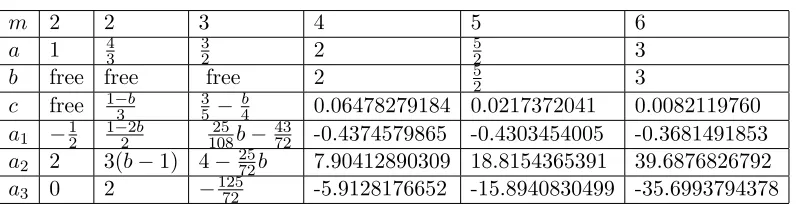
Table 1

m 2 2 3 4 5 6

a 1 4₃ 3₂ 2 5₂ 3

b free free free 2 5₂ 3

c free 1−₃b 3₅− b

4 0.06478279184 0.0217372041 0.0082119760

a1 −1₂ 1−₂2b ₁₀₈25b−43₇₂ -0.4374579865 -0.4303454005 -0.3681491853 a2 2 3(b−1) 4−25₇₂b 7.90412890309 18.8154365391 39.6876826792

a3 0 2 −125₇₂ -5.9128176652 -15.8940830499 -35.6993794378

where

       

      

un= _ff0(₍x_xn)

n),

yn=xn−aun,

νn= _ff0(₍x_yn)

n),

ηn=xn−bun−cνn.

(1.8)

Neta and Johnson [18] give a table of values for the parametersa, b, c, a1, a2, a3 for several values ofm. But, they do not give a closed formula for general case. we list this parameters for m = 2,3,4,5 and 6 in Table 1. Neta [15] has developed another fourth-order method requiring one-function and three-derivative evaluation per iteration. This method is based on Murakami’s method [14] given by

xn+1 =xn−a1un−a2νn−a3w(xn)−ψ(xn) (1.9)

whereun, yn, νn and ηn are given by (1.8) and

w(xn) = f(xn) f0(ηn) ,

ψ(xn) =

f(xn) b1f0(xn) +b2f0(yn)

. (1.10)

A table of values for the parameters a, b, c, a1, a2, a3, b1, b2 for several values ofm is also given by Neta [15].

In [11], Li et al. have proposed a fourth-order method requiring one-function and two-derivative evaluation per iteration. This method is based on the Jarratt method [1] given by the iteration function

  

 

yn=xn−_m2₊₂m _ff0(₍x_xn)

n),

xn+1=xn−

1

2m(m−2)( m m+2)

−m_f0₍_y

n)−m 2

2 f

0₍_x

n)

f0₍_x

n)−(_m+2m )−mf0(yn)

f(xn)

f0₍_x

n).

(4)

In [12], a fourth-order method is proposed,

 



yn=xn−rac2mm+ 2_ff0(₍x_xn)

n),

xn+1=xn−a3_ff0(₍x_yn)

n)−

f(xn)

b1f0(xn)+b2f0(yn)

(1.12)

where

a3 = −

1 2

(_mm₊₂)mm(m4+ 4m3−16m−16)

m3₋₄_m_{+ 8} ,

b1 = −

(m3−4m+ 8)2

m(m4_{+ 4}_m3₋₄_m2₋₁₆_m_{+ 16)(}_m2_{+ 2}_m₋₄₎,

b2 =

m2(m3−4m+ 8)

(_mm₊₂)m₍_m4_{+ 4}_m3₋₄_m2₋₁₆_m_{+ 16)(}_m2_{+ 2}_m₋₄₎.

This method require one-function and two-derivative evaluation per it-eration.

Heydari et al. [13] have developed two fourth-order methods requiring two-function and two-derivative evaluation per iteration. This method is based on Chun fourth-order method (for simple roots) [3] given by the iteration function

 



yn=xn−θi_ff0(₍x_xn)

n),

xn+1 =xn+βi_ff0(₍x_xn)

n) +λi

f(yn)

f0₍_x

n)+δi

f(yn)f0(yn)

f0₍_x

n)2 , i= 1,2,

(1.13) where             

θ1= 1,

β1 =−m3+ 3m2−3m, λ1 =−2m(m−1) m_m−1

−m ,

δ1=m(m−1)2 m_m−1

−2m , (1.14) and                 

θ2 = _m2m₊₁,

β2= 1₄m2−m−1₄.

λ2=−1₄ (m−1) (m+ 1)2

m−1

m+1

−m ,

δ2= 1₄m(m−1)2

m−1

m+1

−2m .

(1.15)

(5)

third-order and fourth-order methods for finding multiple roots of non-linear equations. Each of them requires one evaluation of the function and two of its first derivative per iteration.

2. Development of methods and convergence analysis

Now, we consider the following iteration scheme:

( _y

n=φi(xn, θ),

xn+1 =xn−H(ξn)_ff0(₍x_xn)

n), i= 1,2

(2.1)

whereξn= f 0₍_y

n)

f0₍_x

n),H(t) represents a real-valued function andφi(xn, θ), i=

1,2 are the second-order iteration functions known in the literature(for θ= 1), which are given as follows.

φ1(x, θ) =x−θ

f(x)f0(x)

f2₍_x_{) +}_f02₍_x₎ (2.2)

φ2(x, θ) =x−θf(x)

f0₍_x₎ (2.3)

(2.3) is Newton’s iteration function and (2.2) the iteration function de-rived in [8].

2.1. New third-order schemes free of second derivatives. For simplicity, we define

Aj =

f(m+j)(α)

f(m)₍_α₎ , j = 1,2,· · · , µ= m−θ

m (2.4)

we consider the following iteration functions

( _y

n=φ1(xn, θ),

n),

(2.5) We can state the following convergence theorems for the two-step method defined by (2.5).

Theorem 2.1. Let α ∈ I be a multiple root of multiplicity m of suf-ficiently differentiable function f :I −→ R for an open interval I and H1(t) be a real-valued function as follows

(6)

If x0 is sufficiently close to α, then the method defined by (2.5) has third-order convergence, when

a1 = −

m −θ2(m+ 1) +θ m+m2

θ(θ(m+ 1)−2m) , (2.7)

b1 =

(m−θ)2m m_m−θ−m

θ(θ(m+ 1)−2m) , (2.8)

and satisfy the error equation

en+1 = [χ1(m, θ)A21+ψ1(m, θ)A2]e3n+O(e4n), (2.9)

where en=xn−α and A1, A2 are defined in (2.4) and

χ1(m, θ) = 1 2

−2m3−6m2+ m3+ 9m2+ 6mθ (−2m+θ(m+ 1)) (m+ 1)2(m−θ)m2

+1 2

−2m2₋₄_m₋₂ θ2

(−2m+θ(m+ 1)) (m+ 1)2(m−θ)m2 (2.10)

ψ1(m, θ) = 2m

2₊ ₋_m2₋₄_m

θ+ (m+ 2)θ2

(−2m+θ(m+ 1)) (m+ 1)m2₍_m_{+ 2)} (2.11)

for anyθ∈R and θ6=m,_m2m₊₁.

Proof. Letα∈Rbe a multiple root of multiplicitymof a sufficiently smooth functionf(x),en=xn−αand ˆen=yn−α, where ynis defined

in (2.5). Using the Taylor expansion of f(xn), f0(xn) and f0(yn) about α, we have

f(xn) =

f(m)(α) m! e

m

n[1 +C1en+C2e2n+C3e3n+C4e4n+O(e5n)], (2.12)

f0(xn) =

f(m)(α) (m−1)!e

m−1

n [1 +D1en+D2e2n+D3e3n+D4e4n+O(e5n)], (2.13)

f0(yn) =

f(m)(α) (m−1)!eˆ

m−1

n [1 +D1eˆn+D2eˆ2n+D3eˆ3n+D4ˆen4 +O(ˆe5n)], (2.14)

whereCj = ₍_mm₊!_j_)!Aj andDj = ₍_m(m₊−_j₋1)!_1)!Aj. From (2.12) and (2.13), we

can get

f(xn) f0₍_x

n)

= en

m[1 + (C1−D1)en+ (C2−D2+D 2

1 −C1D1)e2n

(7)

f(xn)f0(xn) f2₍_x

n) +f02(xn)

= 1 men+

D1+C1

m −2

D1 m

e2_n

+

D2+C1D1+C2

m −

D12+ 2D2+m−2 m

−2(−D1+C1)D1

m )en

3₊_{O e}4

n

(2.16)

So, from (2.16) we have

ˆ

en=en−θ

f(xn)f0(xn) f2₍_x

n) +f02(xn)

=d0en+d1e2n+d2e3n+d3e4n+O(e5n) (2.17)

where

d0 = µ

d1 =

θ (D1−C1) m

d2 =

θ D2m2+m2C1D1−m2C2−D12m2+ 1

m3

d3 =−

θ −D3m2+m2C3−m2C1D2−m2C2D1

m3

−θ 2D1D2m

2₋₃_C

1−D13m2+ 3D1+C1D12m2

m3 By substituting (2.17) into (2.14) , we can get

f0(yn) =

f(m)₍_α₎ (m−1)!e

m−1

n Λ[1 +D1ˆen+D2eˆ2n+D3eˆ3n+D4eˆn4 +O(ˆe5n)], (2.18)

where

Λ = (d0+d1e1n+d2en2 +d3e3n+O(e4n))m

−1

=dm₀−1+ (m−1)dm₀−2d1en+{

m−1 2

d2₁dm₀−3+ (m−1)d2dm0−2}e2n

+{2

m−1

2

d1d2dm0 −3+ (m−1)d3dm0−2

+

m−1

3

d3₁dm₀−4}e3_n+O(e4_n). (2.19)

Dividing (2.14) by (2.13), we have

ξn= f0(yn) f0₍_x

n)

=µm−1−θ µ m−2_D

1(µ−m+ 1) +µm−2C1(m−1)

en

m +O e

2

n

.

(8)

Now from (2.5), (2.6), (2.15) and (2.20) we have

en+1 =en−H1(ξn) f(xn) f0₍_x

n)

=K1en+K2e2n+K3e3n+O(e4n), (2.21)

where

K1 =−

−m+a1+b1µm−1

m , (2.22)

K2 =−

b1µm−2(θ m−θ−µ m−µ θ−µ mθ)−a1m

A1

m3₍_m_{+ 1)} (2.23)

Before we listK3, we choose a1 and b1 to annihilate the coefficientsK1 and K2, so we have

a1 = −

m −θ2(m+ 1) +θ m+m2

θ(θ(m+ 1)−2m) , (2.24)

b1 =

(m−θ)2m m_m−θ−m

θ (θ (m+ 1)−2m) , (2.25)

By substituting (2.24) and (2.25) intoK3, we get

K3=χ1(m, θ)A21+ψ1(m, θ)A2, (2.26)

where

χ1(m, θ) = 1 2

−2m3−6m2+ m3+ 9m2+ 6mθ (−2m+θ(m+ 1)) (m+ 1)2(m−θ)m2

+1 2

−2m2−4m−2θ2

(−2m+θ(m+ 1)) (m+ 1)2(m−θ)m2 (2.27)

ψ1(m, θ) = 2m

2₊ ₋_m2₋₄_m

θ+ (m+ 2)θ2

(−2m+θ(m+ 1)) (m+ 1)m2₍_m_{+ 2)} (2.28) and θ6=m,_m2m₊₁. Therefore, we have

en+1= [χ1(m, θ)A21+ψ1(m, θ)A2]e3n+O(e4n), (2.29)

which indicates that the order of convergence of the methods defined by (2.5) is at least three. This completes the proof.

H2(t) = 1 a2+b2t

(9)

a2 =

m2−3θ m+ (m+ 1)θ2

mθ (θ (m+ 1)−2m) , (2.31)

b2 = −

(m−θ)2 m_m−θ−m

mθ (θ (m+ 1)−2m), (2.32)

χ2(m, θ) = 1 2

−2m2−2m+ m2+ 7mθ+ (−2m−2)θ2

m(θ m−2m+θ) (m+ 1)2(m−θ) , (2.34)

ψ2(m, θ) = 2m

2₊ ₋_m2₋₄_m

θ+ (m+ 2)θ2

(−2m+θ(m+ 1)) (m+ 1)m2₍_m_{+ 2)} (2.35) for anyθ∈R and θ6=m,_m2m₊₁.

Proof. The proof method is similar to the Theorem 2.1’s, it’s easy so omit.

H3(t) = 1 + a3t 1 +b3t

. (2.36)

a3 =

θ (m−1) m_m−θ−m m2θ−2m2+ 2m−θ

m3 , (2.37)

b3 = −

m−θ m

−m

m3₊_m2_θ₋_θ2_m2₋₂_{θ m}₊_θ2

m3 (2.38)

χ3(m, θ) = 1 2

η(m, θ)

(m+ 1)2(m−θ)m3₍_{θ m}2₋₂_m2_{+ 2}_m₋_θ₎, (2.40)

ψ3(m, θ) = 2m

2₊ ₋_m2₋₄_m

θ+ (m+ 2)θ2

(10)

η(m, θ) =−2m5+ 6m3+ m5−m3−14m2+ 6m4θ + −8m3−2m4+ 4m2+ 10m

θ2+ 2m3+ 2m2−2m−2 θ3 (2.42)

for anyθ∈R and θ6=m,_m2m₊₁.

Proof. The proof is similar to that of Theorem 2.1’s, so it’s omitted. 2.2. New fourth-order schemes free of second derivatives. Now we consider the following iteration functions

( _y

n=φ2(xn, θ),

n),

(2.43)

We can state the following convergence theorems for the two-step method defined by (2.43).

H4(t) =a4+b4t+c4 t2

2. (2.44)

If x0 is sufficiently close to α, then the method defined by (2.43) has fourth-order convergence, when

θ = 2m

m+ 2 (2.45)

a4 = 1

8m m

3_{+ 6}_m2_{+ 8}_m_{+ 8}

, (2.46)

b4 = −

1 4m

3₍_m_{+ 3)}

m m+ 2

−m

, (2.47)

c4 = 1 4m

4

m m+ 2

−2m

(2.48)

en+1 =K4e4n+O(e5n), (2.49)

where en=xn−α and the error constant K4 is given by

K4 = 1 3

m4_{+ 2}_m3_{+ 2}_m2₋₂_m_{+ 12}

(m+ 1)3m5 A

3 1−

A1A2

m(m+ 2) (m+ 1)2

+ mA3

(11)

Proof. From (2.15) and (2.43) we have ˜

en=en−θ f(xn) f0(xn)

=p0en+p1e2n+p2en3 +p3e4n+O(e5n), (2.51)

where

p0 = µ, (2.52)

p1 = −

θ(C1−D1)

m , (2.53)

p2 = −

θ(C2−D2+D12−C1D1)

m , (2.54)

p3 = −

θ(C3−D3+ (D1−C1)D2 m

− θ(D2−C2+C1D1−D

2 1)D1)

m . (2.55)

and

f0(yn) =

f(m)(α) (m−1)!e˜

m−1

n [1 +D1e˜n+D2e˜2n+D3˜e3n+D4˜e4n+O(˜e5n)], (2.56)

By substituting (2.51) into (2.56) , we can get

f0(yn) =

f(m)(α) (m−1)!e

m−1

n ∆[1 +D1e˜n+D2˜e2n+D3e˜3n+D4e˜4n+O(˜e5n)], (2.57)

where

∆ = (p0+p1e1n+p2e2n+p3e3n+O(e4n))m−1

=pm₀ −1+ (m−1)pm₀−2p1en+{

m−1 2

p2₁pm₀−3

+ (m−1)p2p0m−2}e2n+{2

m−1 2

p1p2pm0−3+ (m−1)p3pm0−2

+

m−1

3

p3₁pm₀−4}e3_n+O(e4_n). (2.58)

Now from (2.15), (2.20), (2.43) and (2.44) we have

en+1 =en−H4(ξn) f(xn) f0(xn)

=K1en+K2e2n+K3en3 +K4e4n+O(e5n), (2.59)

where

K1=− 1

2m 2a4+ 2b4µ

m−1₊_c

4µ2m−2−2m

(12)

K2={ 1

(m+ 1)m2a4+

µm−1θ m+µm−1θ−µm−2θ m+µm−2θ+µm−1m

(m+ 1)m3 b4

+ 1 2

2µ2m−2θ m+ 2µ2m−2θ−2µ2m−3θ m+ 2µ2m−3θ+µ2m−2m

(m+ 1)m3 c4}A1

(2.61)

Before we listK3, we choose a4 and b4 to annihilate the coefficientsK1 and K2, so we have

a4=−

1

2 (µ−m+mµ+ 1)θ{θ (m−1)µ

2m−2₋₍_m_{+ 1)}_µ2m−1 c4

+ (−2µ m2+ 2m2−2µ m2−2m−2mµθ} (2.62)

b4=−

1

(µ−m+mµ+ 1)θ{m

2_µ2−m_{+ (}_θ₍₍_m_{+ 1)}_µm_{+ (1}₋_m₎_µm−1₎_c

4}. (2.63)

By substituting (2.62) and (2.63) intoK3, we get

K3=

ϕ1(θ, m, c4)

2 (m+ 1)2m5_µ ₍₋_m₊_µ₊_mµ_{+ 1)}A 2 1

+ ϕ2(θ, m)

m2₍_m_{+ 1) (}_m_{+ 2) (}₋_m₊_µ₊_mµ_{+ 1)}A2, (2.64)

ϕ1(θ, m, c4) =−

θ2(µm)2(µ+ 1 +mµ−m)3

µ3 c4

+m2 2µ θ−2µ m2θ+ 2mµ−2µ m2+ 4µ2m2

+ 4µ2m+m2θ−3mθ+ 2θ (2.65)

ϕ2(θ, m) =µ(−2m+θ m+ 2θ). (2.66)

Now we choose θ and c4 to annihilate the coefficients ϕ1(θ, m, c4) and ϕ2(θ, m) in K3, so we can get

θ= 2m

m+ 2 (2.67)

and

c4 = 1 4m

4

m m+ 2

−2m

(2.68)

By substituting (2.67) and (2.68) into (??) and (2.63), we get a4 =

1

8m m

3_{+ 6}_m2_{+ 8}_m_{+ 8}

(2.69)

b4 = −

1 4m

3_{(3 +}_m₎

m m+ 2

−m

(13)

Substituting (2.67)-(2.70) into (2.59), we can get the error equation

en+1 =K4e4n+O(e5n), (2.71)

where

K4 = 1 3

m4+ 2m3+ 2m2−2m+ 12

(m+ 1)3m5 A

3 1−

A1A2 m(m+ 2) (m+ 1)2

+ mA3

(m+ 3) (m+ 2)3(m+ 1). (2.72)

which indicates that the order of convergence of the methods defined by (2.43) is at least four. This completes the proof.

H5(t) =

1 a5+b5t+c5t2

. (2.73)

θ = 2m

m+ 2 (2.74)

a5 = 1 16

m4+ 2m3−8m2−16m+ 16

m , (2.75)

b5 = −

1 8

m m+ 2

−m

m m2−6, (2.76)

c5 = 1 16m

2₍_m₋₂₎

m m+ 2

−2m

(2.77)

en+1 =K4e4n+O(e5n), (2.78)

K4 = 1 3

m4_{+ 2}_m3_{+ 5}_m2₋₁₄_m_{+ 12}

(m+ 1)3m5 A

3 1−

A1A2

m(m+ 2) (m+ 1)2

+ mA3

(m+ 3) (m+ 2)3(m+ 1). (2.79)

Proof. The proof is similar to that of Theorem 2.4’s, so it’s omitted.

(14)

H6(t) be a real-valued function as follows

H6(t) =

a6+b6t 1 +c6t

. (2.80)

θ = 2m

m+ 2 (2.81)

a6 = −

1 2m

2_, _(2.82)

b6 = 1 2m

m m+ 2

−m

(m−2), (2.83)

c6 = −

m m+ 2

−m

(2.84)

en+1 =K4e4n+O(e5n), (2.85)

K4 = 1 3

m3_{+ 2}_m2_{+ 2}_m₋₂ (m+ 1)3m4 A

3 1−

A1A2

m(m+ 2) (m+ 1)2

+ mA3

(m+ 3) (m+ 2)3(m+ 1). (2.86)

Proof. The proof is similar to that of Theorem 2.4’s, so it’s omitted.

H7(t) =

a7+t+b7t2 c7+t

(15)

θ = 2m

m+ 2 (2.88)

a7 =

1 4

m5+ 2m4+ 2m3−4m2−16

m m+2

m

m2₍_m_{+ 3)} , (2.89)

b7 =− 1 4

m m+2

−m

m m2−2m+ 2

m+ 3 (2.90)

c7 =−

m m+2

m

m4+ 3m3+ 2m2−4m+ 4

m3₍_m_{+ 3)} (2.91)

en+1 =K4e4n+O(e5n), (2.92)

K4 = 1 3

m7_{+ 4}_m6_{+ 8}_m5_{+ 4}_m4₋₄_m3₋₂₀_m2_{+ 28}_m₋₂₄ (m+ 1)3m5₍₂_m₊_m3_{+ 2}_m2₋₂₎ A

3 1

− A1A2

m(m+ 2) (m+ 1)2 +

mA3

(m+ 3) (m+ 2)3(m+ 1).

(2.93)

Proof. The proof is similar to that of Theorem 2.4’s, so it’s omitted. Remark 2.8. From Theorem (2.6) we can see the method defined by (2.43) withH6(t) is the equivalent to the method (1.11).

Remark 2.9. Any method of the family (2.43) uses three evaluations per iteration, and has fourth-order convergence with conditions of Theorem 2.4-2.7, which accord with the conjecture of Kung-Traub that a multi-point iteration without memory based onnevaluations achieves optimal convergence order 2n−1 forn= 3.

Remark 2.10. Per iteration the presented method requires one evaluation of the function, two of its first derivative. We consider the definition of efficiency index [24] as pw1, where p is the order of the method and

w is the number of function evaluations per iteration required by the method. If we assume that all the evaluations have the same cost as function one, we have that the presented method has the efficiency index I = √34 ' 1.587, which is better than I = √22 ' 1.414 of Newtons method,I = √3

(16)

3. Numerical Examples

In this section, some numerical test of some various multiple-root-finding methods as well as our new methods and Newton’s method are presented. All computations were done using the MAPLE 13 with 128 digit floating point arithmetics(Digits: = 128).We use the following func-tions, which have also been considered in [2, 4, 17].

f1(x) = (x3+4x2−10)3, m= 3, x∗ = 1.3652300134140968457608068290,

f2(x) = (sin2x−x2+1)2, m= 2, x∗= 1.4044916482153412260350868178,

f3(x) = (x2−ex−3x+2)5, m= 5, x∗ = 0.25753028543986076045536730494,

f4(x) = (cosx−x)3, m= 3, x∗ = 0.73908513321516064165531208767,

f5(x) = (xex2−sin2x+3 cosx+5)4, m= 4, x∗ =−1.2076478271309189270094167584,

f6(x) = (sinx−x

2)

2_{, m}_{= 2}_{, x}

∗ = 1.8954942670339809471440357381,

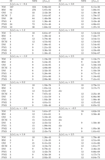
We present some numerical test results for various cubically conver-gent iterative schemes in Table 1. Compared were the Newton method (1.1)(NM), the method of Halley-like method (1.3) (HM),Osada’s method (1.4) (OM), Euler-Chebyshev method (1.2) (ECM), Dong’s method (1.6) (DM) and the methods (2.5) withH1(t) and θ=−1 (PM1), (2.5) with H2(t) and θ = −1 (PM2) and (2.5) with H2(t) and θ = −1 (PM3), respectively, introduced in the present contribution.

Table 1 shows the number of iterations (IT) required such that|f(xn)|<

10−32, the number of function evaluations(NFE) and the values of|f(xn)|.

The test results in Table 1 show that for most of the functions we tested, the methods introduced in the present presentation have at least equal performance compared to the other third-order methods, and can also compete with Newtons method.

We also present some numerical test results for various quartically con-vergent iterative schemes in Table 2. Compared were Newton’s method (1.1)(NM), Neta method (1.7) (NEM)(with b = 0), Li et al’s method (1.12)(LM), Heydari et al’s method (1.13) and (1.14) (HEM1), Heydari et al’s method (1.13) and (1.15) (HEM2) and the methods (2.43) with H4(t) (PM4), (2.43) with H5(t) (PM5), (2.43) with H6(t) (PM6) and (2.43) withH7(t) (PM7), respectively, introduced in the present contri-bution. We used the same test functions as in the test for the above cubically convergent methods.

Table 2 shows the number of iterations required such that |f(xn)| <

(17)

Table 1. Comparison of various third-order convergent

iterative methods and Newton’s method (’div’ means di-vergent)

IT NFE |f(xn)| IT NFE |f(xn)|

f1(x), x0=−0.4 f1(x), x0= 3.0

NM 167 334 6.86e-63 6 12 6.11e-56 HM 92 276 5.87e-92 4 12 1.08e-81 OM 11 33 2.43e-38 4 12 1.30e-46 ECM 7 21 5.81e-97 4 12 1.79e-57 DM 28 84 1.40e-98 4 12 1.28e-84 PM1 4 12 1.36e-46 4 12 3.43e-48 PM2 24 72 6.21e-46 4 12 4.86e-61 PM3 10 30 1.68e-52 4 12 1.37e-55

f2(x), x0= 1.2 f2(x), x0= 2.0

NM 5 10 6.61e-47 6 12 5.12e-64

HM 3 9 1.49e-42 4 12 7.43e-77

OM 4 12 5.78e-46 4 12 3.54e-51 ECM 4 12 4.55e-92 4 12 1.53e-63

DM 3 9 1.08e-45 4 12 5.54e-85

PM1 3 9 1.21e-33 4 12 1.13e-58 PM2 3 9 3.36e-50 4 12 4.33e-69 PM3 3 9 1.38e-45 4 12 9.94e-67

f3(x), x0=−1.0 f3(x), x0= 2.5

NM 4 8 1.19e-59 5 10 1.12e-71

HM 2 6 5.24e-35 3 9 3.44e-50

OM 3 9 2.18e-85 4 12 5.59e-101

ECM 3 9 4.89e-89 3 9 9.27e-35

DM 2 6 2.32e-35 3 9 1.33e-59

PM1 3 9 5.28e-88 3 9 8.77e-41

PM2 3 9 2.81e-86 3 9 1.18e-62

PM3 3 9 2.99e-90 3 9 7.41e-81

f4(x), x0= 0.2 f4(x), x0= 2.5

NM 5 10 1.59e-76 5 10 2.79e-51

HM 3 9 1.85e-54 4 12 3.17e-71

OM 4 12 9.41e-97 div

ECM 3 9 7.67e-42 4 12 2.25e-48

DM 3 9 1.41e-59 4 12 6.86e-90

PM1 3 9 1.93e-39 4 12 1.90e-40 PM2 3 9 4.01e-51 4 12 4.37e-62 PM3 3 9 1.02e-46 4 12 6.05e-55

f5(x), x0=−2.0 f5(x), x0=−0.5

NM 7 14 5.61e-37 9 18 4.62e-53

HM 4 12 1.61e-61 3 9 3.50e-46

OM 5 15 5.10e-45 div ECM 5 15 3.21e-64 div

DM 4 12 2.45e-52 3 9 1.50e-40

PM1 5 15 1.99e-84 div

PM2 4 12 1.58e-86 3 9 1.95e-36 PM3 4 12 2.45e-74 3 9 1.81e-61

f6(x), x0= 1.6 f6(x), x0= 2.5

NM 5 10 1.26e-43 5 10 1.70e-40

HM 3 9 1.12e-35 4 12 4.51e-88

OM 7 21 6.41e-84 4 12 4.41e-66 ECM 4 12 3.18e-72 4 12 1.61e-77

DM 3 9 6.79e-41 3 9 2.46e-33

(18)

Table 2. The number of iterations and NFEs.

f(x) x0 NM NEM HEM1 HEM2 LM PM4 PM5 PM6 PM7

f1 x0= 1.0 6(12) 4(16) 3(12) 3(12) 3(9) 3(9) 3(9) 3(9) 3(9)

x0= 3.0 7(14) 4(16) 4(16) 4(16) 4(12) 4(12) 4(12) 4(12) 4(12)

f2 x0= 1.2 6(12) 4(16) 3(12) 3(12) 3(9) 3(9) 3(9) 3(9) 3(9)

x0= 3.5 7(14) 4(16) 4(16) 4(16) 4(12) 4(12) 4(12) 4(12) 4(12)

f3 x0=−1.0 5(10) 3(12) 3(12) 2(8) 2(6) 2(6) 3(9) 2(6) 2(6)

x0= 4.5 7(14) 4(16) 4(16) 4(16) 4(12) 4(12) 4(12) 4(12) 4(12)

f4 x0= 1.7 5(10) 3(12) 3(12) 3(12) 3(9) 3(9) 3(9) 3(9) 3(9)

x0= 2.5 6(12) 23(92) 4(16) 3(12) 4(12) 4(12) 4(12) 4(12) 4(12)

f5 x0=−3.5 17(34) 10(40) 10(40) 9(36) 9(27) 9(27) 10(30) 9(27) 9(27)

x0=−2.5 11(22) 6(24) 6(24) 6(24) 6(18) 6(18) 6(18) 6(18) 6(18)

f6 x0= 1.7 6(12) 3(12) 3(12) 3(12) 3(9) 3(9) 3(9) 3(9) 3(9)

x0= 2.0 5(10) 3(12) 3(12) 3(12) 3(9) 3(9) 3(9) 3(9) 3(9)

The results presented in Table 2 show that for the considered test func-tions and considered initial guesses the proposed fourth-order methods converge more rapidly than Newton’s method and require the less num-ber of function evaluations, so that they can compete with Newton’s method. Furthermore, for most of the functions we tested, the new methods have at least equal performance when compared to the other well-known classical methods of the same order.

4. Conclusion

In this work, we have suggested two new family of third-order and fourth-order methods for finding multiple roots of nonlinear equations. The presented methods are compared in their performance with var-ious cubically and quartically convergent iteration methods, and it is observed that they have at least equal performance. The result pre-sented in this work can be continuously applied to developing the other cubically and quartically convergent iterative schemes.

References

[1] I.K. Argyros, D. Chen, Q. Qian, The Jarratt method in Banach space setting, J. Comput. Appl. Math. 51 (1994) 103-106.

[2] C. Chun, H. J. Bae, B. Neta, New families of nonlinear third-order solvers for finding multiple roots, Comput. Math. Appli. 57 (2009) 1574-1582.

[3] C. Chun, Iterative Methods Improving Newton’s Method by the Decomposition Method, J. Comput. Math. Appli. 50 (2005) 1559-1568.

[4] C. Chun, B. Neta, A third-order modification of Newton’s method for multiple roots, J. Appl. Math. Comput. 211 (2009) 474-479.

(19)

[6] C. Dong, A family of multipoint iterative functions for finding multiple roots, Int. J. Comput. Math. 21 (1987) 363-367.

[7] E. Hansen, M. Patrick, A family of root finding methods, Numer. Math. 27 (1977) 257-269.

[8] Mamta, V. Kanwar, V.K. Kukreja and S. Singh, On a class of quadratically con-vergent iteration formulae, Appl. Math. Comput. 166(3) (2006) 633-637.

[9] P. Jarratt, Multipoint iterative methods for solving certain equations, Comput. J. 8 (1966) 398-400.

[10] R. F. King, A family of fourth order methods for nonlinear equations, SIAM J. Numer. Anal. 10 (1973) 876-879.

[11] S.G. Li, L.Z. Cheng, A new fourth-order iterative method for finding multiple roots of nonlinear equations, Appl. Math. Comput. 215 (2009) 1288-1292. [12] S.G. Li, L.Z. Cheng, B. Neta, Some fourth-order nonlinear solvers with closed

formulae for multiple roots, Comput. Math. Appli. 59 (2010) 126-135.

[13] M. Heydari, S.M. Hosseini, G.B. Loghmani, Changbum Chun, On some fourth-order nonlinear solvers for finding multiple roots, J. Advan. Research. Appl. Math. 2 (2010) 1-12.

[14] T. Murakami, Some fifth order multipoint iterative formulae for solving equa-tions, J. Inform. Process. 1 (1978) 138-139.

[15] B. Neta, Extension of Murakami’s High order nonlinear solver to multiple roots, Int. J. Comput. Math. (in press).

[16] B. Neta, New Third Order Nonlinear Solvers for Multiple Roots, Appl. Math. Comput. 202 (2008) 162-170.

[17] B. Neta, Numerical Methods for the Solution of Equations, Net-A-Sof, California, 1983.

[18] B. Neta, A. N. Johnson, High-order nonlinear solver for multiple roots, Comput. Math. Appl. 55 (2008) 2012-2017.

[19] N. Osada, An optimal multiple root-finding method of order three, J. Comput. Appl. Math. 51 (1994) 131-133.

[20] E. Schröder, Über unendlich viele Algorithmen zur Auflösung der Gleichungen, Math. Ann. 2 (1870) 317-365.

[21] J. F. Traub, Iterative Methods for the Solution of Equations, Chelsea Publishing Company, New York, 1977.

[22] H. D. Victory, B. Neta, A higher order method for multiple zeros of nonlinear functions, Int. J. Comput. Math. 12 (1983) 329-335.

[23] W. Werner, Iterationsverfahren h¨oherer Ordnung zur L¨osung nicht linearer Gle-ichungen, Z. Angew. Math. Mech. 61 (1981) T322-T324.