Faculty of Electrical Engineering,
Mathematics & Computer Science
Dynamic pricing for camping and bungalow parks:
integer linear programming models for revenue maximization
J.E. Span
MSc Thesis
May 2017
Assesment commitee: prof. dr. M.Uetz (UT) dr. N.Litvak (UT) N.Beimer (Stratech)
Supervisors: prof. dr. M.Uetz (UT) N.Beimer (Stratech)
Abstract
More and more airlines, hoteliers, webshops and other companies apply dynamic pricing strategies to increase their revenue. This project presents a deterministic integer linear program to nd a dynamic pricing strategy to increase revenue of camping and bungalow parks. A simulation framework is proposed to evaluate the performance of a dynamic pricing strategy. The computational experiments are used to validate and test the performance of this linear program. The results show an increase of the revenue relative to the pricing strategy that is currently used by most camping and bungalow parks.
Preface
This thesis is the nal project of my study Applied Mathematics at the University of Twente. I performed my research for the group Discrete Mathematics and Mathematical Programming in the master's program Operations Research.
This project is done in cooperation with Stratech, which develops software for niche markets. Stratech puts industry-specic issues into innovative solutions for (international) organizations which are active in dierent sectors. One of these sectors is the recreation sector, which is the sector of the camping and bungalow parks.
Stratech observes that dynamic pricing is an upcoming research eld. Competitors of Stratech already started small studies to develop tools to support camping and bungalow parks with pricing decisions. Stratech suspect that dynamic pricing will be integrated in the recreation sector soon. Therefore, Stratech also want to start with some studies in this research eld.
Acknowledgements
I have enjoyed working on this project and I want to thank some people who helped and support me during this project.
I would like to thank Niek Beimer who gave me the opportunity to perform my nal assignment at Stratech and being one of my supervisors. He was very helpful on the practical sight of this project. He had the practical knowledge that was needed to come up with an appropriate model. He was always prepared to give me the right data and taking time for brainstorm meetings.
Next I would like to thank Marc Uetz for being my supervisor of this project. He pushed me into the right mathematical direction and our conversations were useful to get positive progress during this project.
I also would like to thank Nelly Litvak who was prepared to take place into the assessment committee and for the time spending on reading and judging my master thesis
I thank Yoeri Boink and Stefan Klootwijk to give up some time for me to listen en help me with some mathematical problems. In special Yoeri, who also was prepared to read my thesis and give me feedback.
Contents
1 Introduction . . . 1
2 Literature review . . . 3
2.1 Dynamic pricing . . . 3
2.2 Demand forecasting . . . 5
3 Modeling . . . 6
3.1 Network revenue management . . . 6
3.2 Demand elasticity . . . 11
3.3 Expected revenue . . . 12
3.4 Performance evaluation framework . . . 13
3.4.1 Performance of a pricing strategy . . . 13
3.4.2 Simulation approach . . . 14
3.4.3 Distinction of expected revenues . . . 16
4 Deterministic integer linear programming . . . 18
4.1 Aggregate expected reservation pricing model . . . 18
4.2 Validation and simulation of the expected revenue . . . 19
4.2.1 Discrete demand simulation . . . 19
4.2.2 Extension of the demand elasticity function . . . 20
4.2.3 Computation of the revenue . . . 21
5 Demand forecasting . . . 25
5.1 Demand model . . . 25
5.2 Monte Carlo simulator . . . 28
5.3 Maximize revenue of Monte Carlo path . . . 29
6 Computational experiments and analysis . . . 30
6.1 Experimental setup . . . 31
6.2 Validation analysis . . . 34
6.2.1 Integrality gap . . . 34
6.2.2 Simulation gap . . . 37
6.3 Performance analysis . . . 39
6.3.1 Revenue improvement . . . 39
6.3.2 Benchmark . . . 40
6.3.3 Computational time . . . 41
6.4 Sensitivity analysis . . . 43
6.4.1 Modied demand elasticity function . . . 43
6.4.2 Modied expected number of requests . . . 45
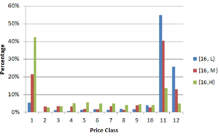
6.5 Practical analysis . . . 47
6.5.1 Unexpected requests . . . 47
6.5.2 Night stay prices . . . 48
7 Critical review . . . 50
8 Summary and recommendations . . . 52
8.1 Summary . . . 52
8.2 Recommendations future research . . . 53
8.3 Recommendations for Stratech . . . 54
1 Appendices . . . 57
A Notation and denitions . . . 57
1 Introduction
The leisure industry is a worldwide active industry. One big part of the leisure industry is the industry that rents campgrounds and bungalows. The companies of this part of the industry can outsource tasks like administration, marketing and the management of bookings. Stratech is a company that develops software for these tasks. Since 1989 Stratech develops innovative software solutions for niche markets and one of these software solutions is Stratech-RCS and around 300 companies, domestically and abroad, use this software package. Currently, the seasonal prices (low, mid and high season) for each accommodation are set at the beginning of the year. Except for discounts, these prices are hold till the end of the year. Stratech observes that more and more airlines, hoteliers, web shops and other companies successfully apply dynamic pricing strategies to increase their revenue. Therefore, Stratech aims to augment Stratech-RCS with a dynamic pricing tool to support camping and bungalow parks with pricing decisions.
In general, a dynamic pricing strategy is a pricing strategy in which businesses set exible prices for products or service based on current market demands. The goal of dynamic pricing is to adjust the price of a product or service on the situation and/or customer to maximize prots. Dynamic pricing has become a more popular research eld since the Airline Deregulation Act of 1978 [20]. The Airline Deregulation Act is the law that deregulated the airline industry in the United States, removing U.S. Federal Government control over such things as fares, routes and market entry of new airlines. The resulting free market has led to an increased number of ights and a decrease of fares. The development of dynamic pricing models has been upcoming since then. Later, computers became faster and big data turned into a popular research eld. All of this led to more sophisticated dynamic pricing algorithms and thereby more companies integrated dynamic pricing strategies [15, chapter 1]. It is most likely that dynamic pricing strategies will soon be applied by camping and bungalow parks.
Dynamic pricing is a form of revenue management, which is the science of managing a limited amount of supply to maximize revenue, by dynamically controlling the price/quantity oered [1, 3, 4, 15]. In terms of business practice, varying prices is often the most natural mechanism for revenue management. Many industries use various forms of dynamic pricing to respond to market uctuations and uncertain demand [15, chapter 9] and pricing is one of the most eective variables that managers can manipulate to encourage or discourage demand. Pricing is not only important from a nancial point of view, but also from an operational point of view. Prices inuence the decision of customers and thereby help to regulate inventory [4]. Furthermore, demand forecasting plays an important role in the revenue management [12,19]. Accurate demand forecasts are crucial to a valuable revenue management, because prices are adjusted using the demand forecast [4,17,19].
A big challenge in dynamically setting prices is the uncertainty in predicting customer behavior. How do customers respond on price changes? What is the customer willing to pay? But even when the answers to these questions are known, it is not directly clear how prices should be adjusted to obtain a higher revenue taking the limited amount of accommodations into account.
In this project we developed an algorithm that computes a dynamic pricing strategy for camping and bungalow parks, which periodically assigns a price class to each possible reservation to max-imize the total expected revenue. The performance of the obtained pricing strategy is evaluated in a developed simulation framework. What this exactly means becomes clear in the remainder of the report.
2 Literature review
A large volume of the literature on dynamic pricing models is focused on the airline and hotel industry. Literature specically on dynamic pricing models for camping and bungalow parks are very scarce. Fortunately, the hotel industry requires to handle the same kind of problem. In particular, the hotel industry faces similar problems in revenue management concerning demand forecast, customer behavior, occupancy, variable lengths of stay and limited and variable accom-modation types. Camping and bungalow parks deviates from the hotel industry on average length of stay, average time between booking date and arrival date, cancellation rate and demand elas-ticity. For example, the average length of stay is close to 11 days in summer, and reservations for summer can occur more than 9 months in advance for early bookers, while the average length of stay in the hotel industry is close to 4 days and most reservation occur less than 3 months in advanced. Some companies allow unsynchronised arrivals (Wednesday, Saturday, Sunday) when others impose Saturday to Saturday stays. Further, camping and bungalow parks have dierent ancillary costs, inventory size, inventory heterogeneity and customer segments. We have focused on the literature of dynamic pricing models concerning the hotel industry and keep in mind these dierences to come up with an appropriate model and solution strategy.
2.1 Dynamic pricing
A clear literature review on dynamic pricing in the hotel industry can be found in [2]. The works [4] and [15] present an overview of dynamic pricing models for revenue management. From these articles we obtained that the dynamic pricing problem is modeled and solved in many dierent ways. The dynamic pricing problem in the hotel industry is usually formulated as a network revenue management problem. In [15, chapter 3] and section 3.1 a description is given of this network. The network revenue management is widely used in the airline industry. However, in contrast to the airline industry, the end of the horizon in not clear in the hotel industry. In the airline industry each ight has a certain departure day, called end of horizon. After this day no seats can be sold. In the hotel industry we do not have such derparture day after no rooms can be sold anymore, there is no clear end of horizon. Rolling horizon procedures are used to solve the problem at a given cut-o date (i.e. end of horizon). To point this out, customers usually can not make a booking before a certain time. For example, if customers can not book longer than 1 year in advance, then the cut-o date is set on one year ahead and after each day the horizon `rolls' one day forward. The work of [10] discusses rolling horizon models and techniques for the hotel revenue management.
Two main solution approaches for the network revenue management problem are deterministic linear programming (LP) and dynamic programming (DP). Generally, LP's generate, if frequently resolved, good pricing strategies. However, the deterministic approach ignores demand uncertainty, which is the main weakness of LP's. A stochastic DP formulation can overcome this weakness, but its state space can easily suer from Bellman's main curse of dimensionality.
A commonly used approach in the DP's is DCOMP, which is a decomposition of the network problem into a set of smaller problems where each concerns only one resource (i.e. a single night stay). A clear introduction to this concept can be found in [15, chapter 4] and examples of the DCOMP approach can be found in [7,13,22,23]. The works [13,15,18] propose strong heuristics for the network revenue management in practice. The works [8] and [22] consider variants of DCOMP and [13] studied both deterministic and stochastic LP in a simulating setting. The DP approach is popular in recent research and shows to generate strong heuristics [24].
The deterministic linear programming approach is one of the traditional approaches for making pricing decisions in network revenue management. This deterministic linear program assumes that the arrivals of customers are given by deterministic functions of the prices. The LP dates back to the work of [9] and it has been widely used by practitioners [8]. The work of [16] proposed a deterministic choice based linear model (CDLP) to solve the network revenue management problem with column generation techniques. In [14] two new method are proposed to solve the CDLP eciently.
Besides the LP and DP approach, another solution approach is proposed in [3]. The authors developed a price optimization framework based on price multipliers. The price is the product of four optimised multipliers (time, capacity, length of stay and group size). Each multiplier varies around one and provides a varying discount or surcharge over some seasonal reference price set by the company. A Monte Carlo simulation from [21] is used for simulating the demand.
2.2 Demand forecasting
A demand forecast in the hotel industry (and camping and bungalow parks) has three dimensions: time of booking, time of arrival and the length of stay. The work of [21] composed two competing philosophies in the forecasting theory. One approach is based on using the historical data to develop an empirical formula for the forecasting variable (number of future arrivals). The other approach focuses on simulating a predened model forward in time to obtain the forecast.
The work of [19] compared several forecasting methods and distingished three forecasting methods: historical booking methods, advanced booking methods and combined booking methods. Methods like moving average, exponential smoothing and other autoregressive models are often used in practice [11]. All these methods are used to develop an empirical formula for the forecasting. The authors of [19] argued that demand forecasting is quite company specic and one needs to be careful by a general usage of a demand forecasting model.
3 Modeling
A dynamic pricing strategy is a pricing strategy in which businesses set exible prices for products or service based on current market demands. The dynamic pricing problem is modeled as a revenue management network. Furthermore, we propose how we model the eect of price changes on demand, called demand elasticity. This demand elasticity is a part of the demand forecasting and, hence, also plays an important role in the dynamic pricing problem. Finally, we present an performance evaluation framework for a dynamic pricing strategy.
3.1 Network revenue management
Camping and bungalow parks typically rent multiple object types (e.g. campground, luxury camp-ground, bungalow, camper ground etc.). We assume that the demand model dier along the object types and that customers do not choose along objects. For example, a customer that intends to book for a bungalow would not search for a campground even when the price of the bungalow is higher than his willing of pay. We model the dynamic pricing problem for a single object type. Furthermore, we model the dynamic pricing problem as a Revenue Management network.
We rst dene a time horizon which denotes the begin and the end of the considered time period.
Denition 1 We deneT ={d1,d2, ...,de} as the time horizon (in days). The rst and last day
of the arrival horizon are denoted byd1 andderespectively.
To remark, de denotes the cut-o date of the time horizon.
Customers arrive on a certain day in the time horizon. However, some camping and bungalow parks allow unsynchronised arrivals (Wednesday, Saturday, Sunday) when others impose Saturday to Saturday stays.
Denition 2 We deneH={a1,a2, ...,ae}as the arrival horizon (in days), where arrivals may
occur. The rst and last day of the arrival horizon are denoted bya1 andaerespectively.
We also dene a set of night stays that can be consumed by the customer. A night stay is the night between two consecutive days. For example, the night of '27-May-2017 on 28-May-2017' and night of '28-May-2017 on 29-May-2017' etc. are night stays.
Denition 3 The set I denotes the set of oered night stays. A single night stay i ∈ I is
denoted by the pair (d,d+1) withd,d+1∈T, whered+1 denotes the day after d.
Horizon
a1 a2 a3
i1 i2 i3
d1 d2 d3 d4 d5 d6 d7
i4
Figure 1: Time horizond1tod7of one week, with allowed arrivalsa1toa3and oered night stays
i1 toi4
Denition 4 We dene La as the set of possible lengths of stay from some arrival daya ∈ H.
Denition 5 A reservation r is denoted by the pair (a,l), with a ∈ H and l ∈ La. The set R={(a,l) |a∈ H,l ∈ La} denotes the set of all possible reservations.
Moreover, consider some reservationr with arrival day a∈ Handl ∈ La, then
{(a,a+1);(a+1,a+2);...;(a+l−1,a+l)} ⊆ I. We use ar to indicate that this is the arrival day
of reservationr andlr to indicate the length of stay of reservationr.
Furthermore, each company has a certain amount of available objects to rent. The number of available objects is called the capacity.
Denition 6 The capacity is dened by c ={c1, ...,cm}, where ci denotes the capacity of night
stayi at the beginning of the decision horizon.
Each reservation consumes a number of night stays. The night stay consumption for all reservations is denoted by the m×n matrix A, with mthe total number of considered night stays and n the total number of reservations.
Denition 7 The m×n matrix Arepresents the night stay consumption of all reservations, where the (i,r)th element, a
i,r, denotes the quantity of night stay i consumed by a reservation r;
ai,r =1 if night stayi is used by reservationr andai,r = 0 otherwise.
Let Ai be theith row of Aand A
r be therth column of A, respectively. To simplify the notation,
we user∈ Ai to indicate that reservationr uses night stayi andi∈ A
r to indicate that night stay
iis used by reservationr.
We are allowed to charge dierent prices of each possible reservation separately. From now on, each possible reservation can be placed in a certain price class and pr denotes the reference price
of reservation r. The reference price is the price established by the company at the beginning of the year or, in other words, the price that is charged if we did not use dynamic prices.
Denition 8 The set K is a non-empty set of integers, called price classes. We dene {pkr |
We require that pr ∈ {pkr | k ∈ K }, which indicates that there is a price class for the reference
price. To give an example, consider three prices classes, i.e. K={1,2,3}. Price class1indicates a 10% discount, price class2follows the reference price and price class 3 indicates a 10% surcharge of the price. Then p1r =0.9·pr, p2r =1·pr (= reference price) andp3r =1.1·pr.
Stratech asks for periodically change of prices. Hence, price changes may occur at dierent time points and can hold for a certain time period. Therefore, we dene the decision periods. A decision period is a certain time period of at least one day (e.g. day or week) and at the beginning of each decision period prices can be changed which are hold till the end of the decision period.
Denition 9 We dene D = {w1,w2, ...,we} as the set of decision periods with w1 the rst
decision period and wethe last decision period. We dene dw1 ∈T anddwe ∈T as the rst and last
day of decision period w respectively. Prices are charged at the beginning of d1
w and holds till the
end of dwe.
To clarify, consider some decision period w, then prices of all reservationr with ar ≥ dw1 can be
changed, i.e. arrival dayar is later (or on the same day) in the time horizon than the rst day of
decision periodw. A request can be made on a certain day before arrival. Moreover, a request for
reservationr can be received in each decision period wif ar ≤dew. Each request that is received
in decision period w for a reservationr with ar ≥dw1 is oered for the price pkr if price class k is
charged for reservationr in decision periodw. Fig 2 illustrates the relation betweenH andD.
de
w1 dw2e
d1
w1 d1w2
a1 a2 a3 a4 a5 a6 a7
w1 w2
r1
r2
r3
r4
Figure 2: Decision period w1 andw2 are periods of ve days. At the beginning of day dw11 we can
charge new prices for all reservation ar ≥dw11, i.e. r1,r2,r3, r4. These prices holds till the end
of daydwe1. At the beginning ofdw12 we can charge new prices for all reservationar ≥dw12, i.e. r2,
Throughout the paper, we reserve d ∈T,a ∈ H,i ∈ I,l ∈ L,r ∈ R,k ∈ K,w∈ D as the indices
for days, arrival days, night stays, length of stay, reservations, price classes and decision period respectively. The following example is used to illustrate the network revenue management.
Example 1 Consider a small bungalow park which decide to start changing prices for his accom-modations on Monday 8th of May, 2017. The week Monday May 22th to Sunday May 28th is
the last week of the time horizon and contains the ascension weekend. Thus, the considered time horizon is given by T ={ May 8th, May 9th,...,May 28th}. The park requires that arrivals only
occur in the ascension weekend except for the Sunday, so H ={Friday May 26th, Saturday May
27th }. For shorter notation, H = {a
1,a2} = {Fr,Sa}. Further, a reservation needs to be made
for three night stays if Friday is the arrival day and for at most two night stays if Saturday is the arrival day. Hence, La1 ={3} and La2 ={1,2}. The park requires weekly price changes, so
D={w1,w2,w3}={May 8th - May 14th),(May 15th - May 21th),(May 22th - May 28th)}. Thus,
price changes in decision periodw1 occur at the beginning of daydw11 (= May 8th) and are hold till
the end of day dwe1 (= May 14th). The same principle holds for periods w2,w3. The set of oered
night stays that can be consumed by the customer is given byI={(Fr,Sa),(Sa,Su),(Su,M o)}.
As-sume that the park has only 3 accommodations available for the ascension weekend, i.e. c={3,3,3}.
Now, the night stay consumption matrix Ais given by
A= ©
«
r1 r2 r3
(Fr,Sa) 1 0 0
(Sa,Su) 1 1 1
(Su,M o) 1 0 1 ª ® ® ®
¬
and the set of considered reservation becomesR ={(Fr,3),(Sa,1),(Sa,2)}. See g 3 for a
visualiza-tion ofH,DandRand considerr1=(Fr,3),r2=(Sa,1),r3=(Sa,2). Assume priceprk3 is charged
for reservation r3 in decision period w1 and one request for r3 is received in decision period w1.
There is enough capacity, so the request can be accepted and night stays {i|i∈Ar3}are consumed.
The revenue increases with prk3 and the capacity becomes c={3,2,2}.
w
1w
2w
3a
1a
2Fr Sa Su Mo
May 8 May14 May15 May21 May22 May28
r
1r
2r
3The developed ILP uses the expected number of requests for some reservation at a certain price class in a certain decision period. This is the most important input parameter of the ILP proposed in section 4.1.
Denition 10 We denebkr,w as the expected number of requests when price classkis charged in decision period w for reservation r. We dene br,w as the the expected number of requests for
reservation r in decision period w at the reference price. The expected number of request br,w
is represented by a matrix b with the reservations r on the rows and decision periods w on the
columns.
Note that bk
r,w =0 for all k ifar < dw1. We further note thatbkr,w also could be zero if ar ≥dw1,
but that it is possible in practice that reservationr in decision periodwis actually received, even
if it was not expected. This leads to some practical problems, but this is discussed later in more detail in.
We now employ a few assumptions for the expected number of requests. First, we assume that there exist some φ ∈ K such that bφr,w =0. In this case, if there is not enough capacity to serve a request for reservationr, then we charge the (large) price pφr to ensure that we do not receive a request for reservationr in decision periodw. Second, because we use an independent demand
model, we assume thatbkr,w depends only on the price for reservationr in decision periodw, but
not on the prices for the other reservations in decision periodw.
Our goal is to nd a pricing strategy which maximize the revenue of camping and bungalow parks.
Denition 11 A pricing strategy is denoted by the binary vector urk,w, with Í
k∈Kukr,w =1 for
allr ∈ R andw∈ D. Ifurk,w =1 then price class k is charged for reservationr in decision period
w.
In words, a dynamic pricing strategy assigns a single price class in each decision period to each possible reservation.
Denition 12 If k = {k|pr = pkr} and urk,w = 1 for all r and w, then ukr,w is called a static
pricing strategy. Ifukr,w is not a static pricing strategy, thenurk,w is called a dynamic pricing strategy.
In words, a static pricing strategy is the pricing strategy which assigns the price class of the reference price in each decision period to each possible reservation. Then the objective of the network revenue management problem is to nd pricing vectoruk
3.2 Demand elasticity
The demand elasticity is the degree to which demand varies with its price. Camping and bun-galow parks that currently use Stratech-RCS never used dynamic pricing strategies before. As a consequence that there is an insucient amount of data concerning the eect of price changes on demand. Therefore, an assumption needs to be made. We assume that the demand is a linear function of the price. In Chapter 5 we propose a demand model to nd the expected values br,w
and the values bk
r,w are computed by a linear demand elasticity function. Usually, the demand
decreases when the price increases and visa versa. Within this project, the demand elasticity function is modeled as a linear price class dependent function, denoted by DE(k). Note that
a more sophisticated demand elasticity might be more appropriate in practice. In practice, the demand elasticity probably depends on the seasonality, time of booking and perhaps also on the reservation. The valuesbrk,w are obtained by multiplyingbr,w with the value ofDE(k)that varies
around one. The demand elasticity gives the expected amount of increase or decrease. Hence, a value of DE(k)that is bigger than one indicates an increase of demand and a value smaller than
one indicates a decrease of demand. The demand elasticity function outputs the value 1 if the price class of the reference price is charged. In general,
bkr,w =br,w·DE(k) k∈ K.
In short,br,w is estimated with a demand forecasting model andbrk,w is estimated by the demand
elasticity function. We use the following example to illustrate the demand elasticity model.
Example 2 Consider the setting of example 1. In addition, consider the set of price classes
K = {1,2,3,4}, where price class 1 indicates a 10% discount, 2 indicates the reference price, 3
indicates a 10% surcharge and 4 indicates price class φ. At the beginning of each decision period some price class k∈ K is assigned for each reservationr ∈ R. Assume that the demand forecast
model outputs
b= ©
«
w1 w2 w3
r1 2.2 0 1
r2 0 1.8 0
r3 0 0 0.7
ª ® ® ® ¬ .
As an illustration, the expected number of requests in decision period w2 for reservation r2 (i.e.
b2,2) equals 1.8 and equals zero for reservationsr1 andr3. Note that the values are allowed to be
continuous because it is an expected value. Let k ∈ K and consider the array α=[0.9,1,1.1,∞].
α(k)indicates the kth element ofα and consider the demand elasticity function
DE(k)= (
−2α(k)+3 if α(k) ≤1.1
0 if α(k)>1.1 (1)
for all reservationsrand decision period w(see g 4). This demand elasticity indicates that if the
price increases with 10%, then we expect that the demand decreases with 20%. On the opposite, if the price decreases with 10%, then we expect that the demand increases with 20%. Moreover, if price class 4 is charged, then we expect no requests. Thus, if the price is increased with 10% in decision period 2 for reservation r2, thenb32,2=1.8·0.8=1.44. Similarly, the value bkr,w can be
k1 k2 k3 k4
Figure 4: Demand elasticity function DE(k) of example 2
3.3 Expected revenue
If the price for some reservation increases or decreases, then the demand elasticity function outputs an expected decrease or increase of demand. With these expectations the expected revenue can be calculated. The expected revenue is obtained by multiplying the expected number of requests by the price that is charged for the reservation of the request. To point forward, in section 4.1 we propose a ILP to nd the maximum expected revenue. The following example illustrates how DE(k)and the valuesbr,w are used to obtain the expected revenue.
Example 3 Consider the setting of example 2 and assume that the static pricing strategy is applied and the bungalow park now has an innite capacity. The reference price (pr) for reservations r1,
r2 andr3 are¤150,-,¤50,- and¤100,- respectively. With matrixbfrom example 2 and prices pr
the expected revenue (E[Rev]) is computed by
E[Rev]= Õ
w∈ D
Õ
r∈ R
br,wpr
=b1,1pr1+b2,2pr2+b1,3pr1+b3,3pr3
=(2.2·150)+(1.8·75)+(1·150)+(0.7·100)=¤640. (2)
In addition, consider the following two pricing strategies. In the rst strategy the price is decreased with 10% for each reservation at the beginning of each period. In the second strategy the price is increased with 10% for each reservation at the beginning of each period. The expected revenue of the rst strategy is computed by
E[Rev]= Õ
w∈ D
Õ
r∈ R
DE(1) ·br,w·0.9pr =
Õ
w∈ D
Õ
r∈ R
1.2·br,w ·0.9pr =¤720.
The expected revenue of the second strategy is computed by
E[Rev]= Õ
w∈ D
Õ
r∈ R
DE(3) ·br,w·1.1pr =
Õ
w∈ D
Õ
r∈ R
0.8·br,w ·1.1pr =¤480.
previous example shows that the optimal expected revenue is easily found with an innite capacity, but in practice there is a capacity constraint. In section 4.1 we proposed a ILP which takes into account this capacity constraint and solves these kind of instances in general. The ILP nds the right trade o between price surcharge and change in demand, given the available capacity. The ILP nd the optimal expected revenue and the output variables are used as a dynamic pricing strategy.
3.4 Performance evaluation framework
Eventually we want to evaluate the performance of the pricing strategy of this algorithm relative to the static pricing strategy that is currently used by most of the companies. In this section we discuss the practical problems that arise in the evaluation of the performance of a pricing strategy and how we overcome these problems.
3.4.1 Performance of a pricing strategy
In practice, the performance of a pricing strategy could be obtained with a practical experiment. For example, we could test the performance of two pricing strategies on two comparable bungalow parks in the same time period. One bungalow park applies a price strategy and the other bun-galow park applies the other pricing strategy in the same time period. At the end both revenues can be compared to evaluate the performance of both pricing strategies. Such practical experi-ment was not suitable for this project and we developed a method to evaluate the performance computationally.
It would be easy if the expected revenue of several pricing strategies can be evaluated as in example 3 and that we can claim that the pricing strategy with the highest expected revenue performs the best. But note that the capacity is innite in this example and that the expected revenue of a pricing strategy is meaningless if the capacity constraint in not taken into account. To explain, consider the setting of example 3, but now with a nite capacity c={3,3,3}. With equation (2)
we computed the expected revenue of¤640 when the static pricing strategy will be applied. But note thatr1,r2 andr3all consumes night stay (Sa,Su) and in the coming three weeks we expect
3.4.2 Simulation approach
The developed simulation framework nds a, so called simulated expected revenue, for a pricing strategy. This revenue is computed in a simulated way and the global idea of the simulation is described below. We assume that the pricing strategy with the highest simulated expected revenue has the best performance.
Global idea simulation approach Simulate future requests (also called demand) for some time and arrival horizon. Manage each request in chronological order and check if the reservation of this request does not violate the capacity. If the request ts and can be accepted, then the total simulated expected revenue increases with the price suggested by the pricing strategy for this request and the available capacity is updated. If the request can not be accepted, then the request is denied and the total simulated expected revenue does not increase.
The simulation experiment sounds accessible, but if price changes are made we also need to predict the behavior of the customers on these changes and some practical problems arise. Moreover, the demand should change somehow due to the price changes and we need to predict the expected future requests that would have occurred if we had used a certain pricing strategy. For example, assume that we generated a future request for some reservation r in decision period w. The
customer of this request will behave dierently on dierent prices for reservationr. What would this customer do if we charge the reference price or increase the price of the reservation? We modeled the customers behavior on prices with the same demand elasticity model as used for the expected number of requests. The expected increase or decrease due to the demand elasticity function is now applied on single request. For example, if we receive a request and price class k is charged and DE(k) = 1.2 then we expect an amount of 1.2 of this request. Similarly, if DE(k) =0.8, then we expect an amount of 0.8 of this request. If the static pricing strategy is used, then DE(k)=1 and we do not expect an increase or decrease of any requests. Therefore, the simulated expected revenue is easily found by above simulation for the static pricing strategy.
Now we only need to nd the simulated expected revenue of a dynamic pricing strategy. But, if we use a dynamic pricing strategy it becomes more complex, because a practical problem arise here. As we already saw above, if we use the demand elasticity model of section 3.2 we could end up with fractional expected future requests, called continuous demand (also illustrated in example 4). With this continuous demand we can compute the simulated expected revenue in a similar way as described in above simulation approach, but a continuous demand is not realistic. In practice customers just accept or deny the price of a reservation. In section 4.2.1 we propose how we obtain a demand in which each customer just accepted or denies the price of a reservation. We employ a few more denition before we illustrate a continuous demand with an example.
Denition 13 A demand stream Q is a set of chronological ordered simulated requests. We deneq(n)=(r,w)as thenth request of demand streamQwhich denotes the request for reservation r and is received in decision period w.
Denition 14 We dene qr,w ∈Q as the total number of realized requests for reservation r
in decision period w in demand stream Q. The values qr,w are represented by the matrix q with
the reservations on the row and decision periods on the columns.
Example 4 Consider the setting of example 3 and assume we have a demand stream Q={q(1), ...,q(5)}={(r1,w1),(r1,w1),(r2,w2),(r3,w3),(r1,w3)} (see g 5). Thus, we consider
b=
w1 w2 w3
r1 2.2 0 1
r2 0 1.8 0
r3 0 0 0.7
and q=
w1 w2 w3
r1 2 0 1
r2 0 1 0
r3 0 0 1
.
As an illustration, we expected1.8requests for reservationr2in decision periodw2and we actually
received 1 request for reservation r2 in decision period w2, which is denoted by q(3) (or q2,2). If
the static pricing strategy is applied on this demand stream, then the simulated expected revenue (E[SimRev]) is computed by
Esim[Rev]=
Õ
w∈ D
Õ
r∈ R
br,wpr =2·150+1·50+1·100+1·150=¤600.
When the price is decreased with 10% for each reservation at the beginning of each period, then the simulated expected revenue is computed by
Esim[Rev]=
Õ
w∈ D
Õ
r∈ R
DE(1) ·qr,w·0.9pr=
Õ
w∈ D
Õ
r∈ R
1.2·qr,w·0.9pr=¤768 (3)
And we obatin a continuous demand stream Qu = {1.2·q(1), ...,1.2·q(5)} = {1.2· (r
1,w1),1.2·
(r1,w1),1.2· (r2,w2),1.2· (r3,w3),1.2· (r1,w3)}. This means that qu(n) ∈Qu now consumes 1.2 of
the capacity instead of 1 on the night staysi ∈Ar with r the reservation of request q(n). Thus, if
we apply a pricing strategy on demand streamQ, then we could end up with a continuous demand streamQu.
Fr Sa Su Mo
a1 a2
r1 r2 r3 r1 r1 q(1) q(2) q(3) q(4) q(5)
Figure 5: Visualization of demand streamQfrom example 4
Note that we can perform the computation in equation (3), because we still have an innite capacity. In section 4.2.3 we propose how Esim[Rev]is computed with a nite capacity.
3.4.3 Distinction of expected revenues
The intended purpose of the simulated expected revenue is that it represents a realistic performance of a dynamic pricing strategy.
Denition 16 We dene Q˜u as the discrete demand stream computed from the (possibly)
continuous demand streamQu.
In section 4.2.1 we propose a method to obtain a discrete demand streamQ˜u from a continuous
demand streamQu.
We now formulate three dierent expected revenues, which are used in the remainder of this report. We rst obtain an expected revenue using pricing vectorukr,w and values bkr,w andpkr as proposed in example 3. Second, we obtain a simulated expected revenue using pricing vector urk,w and a possibly continuous demand streamQu and pricespkr as proposed in example 4. Third, we obtain a, so called, realistic expected revenue using pricing vectorurk,w and a discrete demand streamQ˜u and pricespkr.
Denition 17 The expected revenue E[Rev]is the revenue obtained using some pricing vector
urk,w, expected requests bkr,w and prices pkr.
Denition 18 The simulated expected revenueEsim[Rev]is the revenue obtained using using
some pricing vectoruk
r,w, demand streamQu and prices pkr.
Denition 19 The realistic expected revenue Er eal[Rev] is the revenue obtained using some
pricing vector ukr,w, demand streamQ˜u and prices pkr.
In section 4.2.3 we describe how E[Rev], Esim[Rev]andEr eal[Rev]are actually computed.
Eventually we want to validate that the simulated expected revenue is a good approximation of the realistic expected revenue, because we assume that this realistic expected revenue gives a better representation of the practice. Therefore, we dene the following.
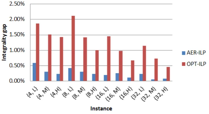
Denition 20 The integrality gap (Gint) is the relative dierence between the simulated
ex-pected revenue of demand stream Q and the average realistic expected revenue (Er eal[Rev]) over
all discrete demand stream Q˜u obtained fromQu.
The integrality gap of a pricing strategy is computed by
Gint =
|Er eal[Rev] −Esim[Rev] |
Esim[Rev]
·100% (4)
Note that there is no integrality gap of the static pricing strategy, becauseEsim[Rev]=Er eal[Rev]
Now it is also important to know how the expected revenue of the ILP and the simulated expected revenue relates. Therefore, we dene the following.
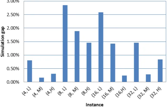
Denition 21 The simulation gap (Gsim) is the relative dierence between the expected
rev-enue and the average simulated expected revrev-enueEsim[Rev]over all (possibly) continuous demand
streamsQu.
The simulation gap is computed by
Gsim=
|Esim[Rev] −E[Rev]|
E[Rev] (5)
4 Deterministic integer linear programming
In this section we propose a deterministic integer linear program (ILP) to nd a dynamic pricing strategy which periodically assigns a single price class to all possible reservations to maximize the expected revenue. Further, a method is proposed to compute a discrete demand stream from a continuous demand stream. Next, we propose and tackle some practical problems that occur and propose the method that is used to compute the simulated and realistic expected revenue. Finally we propose two additional solution approaches which make use of the ILP solution.
4.1 Aggregate expected reservation pricing model
The expected number of requests bkr,w is used to nd the optimal price class for each reservation r for every decision periodw. The expected revenue is maximized with ILP (6) - (9) which nds
the right trade o between price surcharge and change in demand, given the available capacity. The maximum expected revenue is found by assigning a single price class to each reservation r at the beginning of decision period w taking into account that the capacity ci is not violated
for all night staysi ∈ I. This problem is formulated as a deterministic integer linear program,
which we call aggregated expected reservation integer linear program (AER-ILP). It is called the aggregated expected reservation ILP because a price class is assigned to each possible reservation separately and is based on the expected valuesbkr,w. The dynamic pricing strategy that maximize the expected revenue is dened byuˆkr,w which are the output variables of the AER-ILP.
max Õ
w∈ D
Õ
r∈ R ar≥d1w
Õ
k∈K
ukr,wpkrbkr,w (6)
s.t. Õ
w∈ D
Õ
r∈ R ar≥d1w
Õ
k∈K
ai,rukr,wbkr,w ≤ci ∀i∈ I (7)
Õ
k∈K
ukr,w =1 ∀r ∈ R,∀w∈ D (8)
urk,w ∈ {0,1} ∀r∈ R,∀k∈ K,∀w∈ D (9)
4.2 Validation and simulation of the expected revenue
In section 3.4.3 we argued about the integrality gap due to the continuous demand. In this section we propose the method that is used to compute a (more realistic) discrete demand from a continuous demand and is used to nd this integrality gap. Further, we give an extension of the demand elasticity function, which is needed to overcame some practical problems. Finally, we propose how the simulated and realistic expected revenue are actually computed.
4.2.1 Discrete demand simulation
In section 3.4.2 we illustrated that the demand elasticity function gives a certain expected increase or decrease of requests and we showed that we could end up with a continuous demand stream in the simulation framework. Now we explain how we obtain a discrete demand stream Q˜u from a
fractional demand streamQu.
We computed a discrete demand streamQ˜u from a continuous demand streamQu in a simulated
way. For each q(n) ∈ Qu the following simulation is performed to obtain Q˜u. If price class k is charged for the reservation of requestq(n)andDE(k)<1, then with probabilityDE(k)one request
q(n) is added to Q˜u. If DE(k) < 1, then one request q(n) is added to Q˜u and with probability 1−DE(k)an extra requestq(n)is added toQ˜u. IfDE(k)=1, then one requestq(n)is added toQ˜u. We use the following example to illustrate this simulation of a single requestq(n) ∈Qu discrete demand.
Example 5 Consider request q(2) = 1.2· (r1,w1) from demand stream Qu of example 4. Also
consider the demand elasticity function DE(k) and the set of price classes as in example 2. If we
charge price class 3for reservationr1 in decision period1, thenDE(3)=0.8 and the customer of
request q(2)accepts the price 1.1·¤150=¤165 with probability DE(k)=0.8 and deny this price with probability (1−DE(k))=0.2. If we charge price class1 for reservationr1 in decision period
1, then DE(1) = 1.2 and we receive an extra identical request with probability 1−DE(k) = 0.2, otherwise we only receiveq(2). If we charge the reference price we just receive requestq(2).
With above simulation we can generate a large number of dierent discrete demand streams ˜
Qu. The simulated expected revenue for each simulated discrete demand stream can be found by algorithm 1 of section 4.2.3 and we can compute Er eal[Rev] by averaging over all simulated
4.2.2 Extension of the demand elasticity function
Before we propose the method that is used to nd the simulated and realistic expected revenue of a certain pricing strategy, an annotation need to be made. The demand elasticity is used to nd the expected number of increase or decrease of demand. Now, it could be the case that demand stream Q does not contain a request for reservation r in decision period w while br,w >0. The
AER-ILP assigned a price class for this request, namely price class k for which uˆk
r,w =1. In the
simulation experiment we want to know if we could have received a request for reservationr if a certain price class is assigned for this reservation. As an illustration of this case, take matrixbin example 4, but now we also expected 2 request for reservationr2in decision periodw1and matrix
q is still the same. In this case,qr2,w1 =0, while we expected 2 request in this week. With current
demand elasticityDE(k)qr2,w1 =0for allk, but if we use a price class which decrease the price for
reservationr in decision periodw1, then we assume that there should be some expectation that
we receive a requestqr,w under this new price. Moreover, we assume that if we did not expect any
request for reservationr in decision periodw andqr,w=0, then we do not expect that we receive
a request for reservationr in decision periodwat any price class.
We extend our demand elasticity function to tackle this problem. We rst propose the following.
Proposition 1 Ifuˆrk,w =1, pkr >pr andqr,w =0 for some k,r and w, thenqur,w=0.
In words, if we did not receive a request for reservationr in decision period w and we increased
the price ofr in decision periodw, then we expect no request for reservationr in decision period
w. Now, if a pricing strategy assigns a price class which decreases the price forr in decision period
w, then their should be some probability that we received a request forr in decision periodw.
Denition 22 If br,w >0 and qr,w =0 for some reservationr and decision period w, then we
call this an unrealized request for reservationr in decision period w.
If a request is an unrealized request then the demand elasticity becomes
DEr0,w(k)= (
(DE(k) −1)br,w ifDE(k) ≥1
0 ifDE(k)<1 (10)
Function (10) states that if we decrease the price of reservation r in decision period w, then we
have an expected increase of a certain percentage, namelyDE(k) −1, of the number of request we did expected (br,w). Using denition 22 and function (10) we propose the following.
Proposition 2 If br,w > 0 and qr,w = 0 for some reservation r in decision period w, then
DE(k)=DEr0,w(k).
Hence, an unrealized request has the potential to become a request if we charge a lower price for the corresponding reservation and decision period. From now on, we state that a demand stream Qalso contains unrealized request. We illustrate this using example 4, if we indeed expected two request for reservationr2in decision periodw1, then we haveQ={q(1), ...,q(6)}={(r1,w1),(r1,w1),
4.2.3 Computation of the revenue
The proposed AER-ILP computes a maximum expected revenue and outputs a pricing strategy vector uˆkr,w. In this section we describe how the simulated and realistic expected revenues are computed for both static and dynamic pricing strategies.
Simulated and realistic expected revenue
The demand elasticity function gives the value one for all reservations r and decision periodsw
if the static pricing strategy is used. Therefore, with the simulation approach we always end up with a (realistic) discrete demand stream. The following algorithm is used to compute Esim[Rev]
(or Er eal[Rev]) of a discrete demand streamQwith pricing strategyukr,w.
Algorithm 1 For n = 1 to |Q| (or |Q˜u|) the following is performed. If request q(n) ∈ Q (or
|Q˜u|) is a realized request and reservation r of this request does not violate the capacity (i.e. if ci−1 ≥0 ∀i ∈ Ar), then Esim[Rev] (or Er eal[Rev]) increases with pkr with k={k|urk,w =1} and
the capacity is updated withci =ci−1 for alli∈Ar. If requestq(n) ∈Q (or |Q˜u|) is an unrealized
request or the reservation of this request does violate the capacity, then this request is denied and Esim[Rev] (orEr eal[Rev]) does not increase
The following example illustrates algorithm 1.
Example 6 Consider the setting of example 4, but now with a slightly dierent expected request matrixb. We now also expected two requests for reservationr2 in decision periodw1. Thus,
b= ©
«
w1 w2 w3
r1 2.2 0 1
r2 2 1.8 0
r3 0 0 0.7
ª ® ® ®
¬
and q= ©
«
w1 w2 w3
r1 2 0 1
r2 0 1 0
r3 0 0 1
ª ® ® ® ¬ .
and demand streamQcontains also an unrealized request, soQ={q(1), ...,q(6)}={(r1,w1),(r1,w1),
(r2,w1),(r2,w2),(r3,w3),(r1,w3)}, where(r2,w1)is the unrealized request. Consider a (nite) capacity
c = {3,3,3} for the bungalow park and a static pricing strategy is applied. Then Esim[Rev] is
computed with algorithm 1 as follows. Start at n =1, so q(1) =(r1,w1) is received at rst. We
obtain that request q(1) ts (i.e. ci −1 > 0 ∀i ∈ Ar1), so the total simulated expected revenue
increases with pr1 = ¤150 and the capacity is updated (c = {2,2,2}). Similarly, q(2) = (r1,w1)
ts, so the total simulated expected revenue increases with pr1=¤150 and the capacity is updated
(c = {1,1,1}). Next, q(3) = (r2,w1) is `received' which is an unrealized request, but the total
simulated expected revenue does not increases, because DE(k) = 1 and DE0
r2,w1(k) = 0. Then,
q(4) =(r2,w2) is received and this request ts, so the total simulated expected revenue increases
withpr2 =¤50and the capacity is updated (c={1,0,1}). Now we obtain that requestq(5)=(r2,w2)
does not t, because ci−1 <0 fori =(Sa,Su) and this request is denied. Also q(6) does not t
anymore. Thus, if we have a nite capacity c = {3,3,3} and use the static pricing strategy we
obtain
It becomes a little bit more complex if Esim[Rev] is computed for a dynamic pricing strategy.
In this case, we also have to deal with the extended demand elasticity function as described in section 4.2.2. The following algorithm is used to nd Esim[Rev]when a dynamic pricing strategy
is applied.
Algorithm 2 For n = 1 to |Q| the following is performed. If q(n) = (r,w) ∈ Q is a realized request, thenDE=DE(k)withk={k|uˆkr,w=1}. Now, If valueDE of does not violate the capacity (i.e. if ci−DE ≥0 ∀i∈ Ar), then Esim[Rev]increases with DE·pkr and the capacity is updated
withci=ci−DEfor alli∈Ar. If requestq(n)is an unrealized request, then DE=DEr0,w. Now, if
this DE does not violate the capacity, then Esim[Rev]increases with DE·prk for k={k|ukr,w =1}
and the capacity is updated.
The following example is used to illustrate algorithm 2.
Example 7 Consider expected request matrix b, demand stream Q and capacity c from example 6. Now a dynamic pricing strategy is applied which assigns price class 1 (decrease price with 10%) for each reservation in each decision period. Esim[Rev] is computed with algorithm 2 as
follows. Start at n = 1, so q(1) = (r1,w1) is received at rst. This is a realized request, so
DE = DE(1) = 1.2. The value DE ts in the capacity (because ci −DE > 0 ∀i ∈ Ar), so
Esim[Rev] increases with 1.2·0.9·pr1 = ¤162 and the capacity is updated (c = {1.8,1.8,1.8}).
Similarly, for q(2)=(r1,w1)we have enough capacity, so Esim[Rev] increases with ¤162 and the
updated capacity becomesc={0.6,0.6,0.6}. Next,q(3)=(r2,w1)is `received' which is an unrealized
request, soDE=DEr0,w(1)=(DE(k)−1)br,w =(1.2−1)·2=0.2. ValueDE=0.2ts in the capacity,
soEsim[Rev]increases with 0.2·0.9·pr2 =¤9 and the updated capacity becomesc={0.6,0.4,0.6}.
Then,q(4)=(r2,w2)is received, which is a realized request withDE=1.2. This request does not t
anymore, because ci−1.2<0 ∀i∈Ar, soEsim[Rev]does not increase and requestq(4)is denied.
Also, requestq(5)andq(6)do not t and are denied. Thus, if we have a nite capacity c={3,3,3}
and use the above dynamic pricing strategy, then the simulated expected revenue is denoted by
Esim[Rev]=2·162+1·9=¤333.
4.3 Additional approaches
In this section we propose two additional solution approaches which come up during this project. The rst solution approach is to use the dynamic pricing strategy obtained from the AER-ILP to dynamically change prices per night stays instead of prices per reservations. The second solution approach is an extension of the dynamic pricing strategy that is obtained from the AER-ILP, which includes price decisions for unexpected requests.
4.3.1 Night stay pricing
In this section we discuss an additional model to nd a pricing strategy which use prices per night stay instead of prices per possible reservation. We developed such model because in the Stratech-RCS software the calculation of the prices for reservations are often based on prices per night stay. This means that the price for some reservation r is computed by summing up the prices of all night staysi∈ Ar.
But, pricing night stays instead of pricing each reservation separately seems a kind of sub-optimal. We argue as follows, a price for night stayihas an eect on the prices of all reservationsr ∈Ai. It is harder to manage the occupancy with a night stay pricing strategy, because if we use night stay prices, then we can not deny single requests by charging a large price like price classφ. To explain, if we use price classφfor a certain night stay, then we have no request for all reservationsr∈ Ai, which is probably undesirable. We attempt to nd an appropriate night stay pricing strategy and in the computational experiments we test this strategy. We now propose two methods to compute a pricing strategy which periodically change night stay prices.
We computed two pricing strategies using night stay prices which are obtained from the output variables of the AER-ILP. We rst divide the price for each reservation by the number of nights that is consumed by this reservation to obtain a night stay price for all night stays{i|Ar}. Next,
we average all night stay pricesiof reservationsr ∈Ai to obtain the price of night stayi.
Denition 23 pi,w is a night stay pricing strategy, where price pi,w is charged for night stay
i in decision periodw.
The night stay pricing strategypi,w is found by
pi,w=
Í
r∈Ai Í
k∈Kuˆkr,wprk
lr
|{r|r ∈Ai}| . (11)
Where|{r|r ∈Ai}|denotes the number of reservation that consumes night stayianduˆrk,w denotes the output variables of the AER-ILP. Further, we dene p∗r,w as the price for reservation r in decision periodw that is obtained from the night stay pricing strategy and is computed by
p∗r,w= Õ
i∈Ar
Now, Esim[Rev]is computed in a quite similar way as algorithm 2 of section 4.2.3, but we rst
need to mention the following. There are no price classes for reservation anymore, but just prices p∗r,w. Therefore, the price class dependent demand elasticity function can not be used here. To overcome this, a linear demand elasticity function is used, which has the same linear slope as the price class dependent elasticity function. This demand elasticity function is based on function (1) of section 3.2. We consider
DE(p∗r,w)=−2p
∗ r,w
pr +
3 (13)
with extended demand elasticity function
DEr0,w(p∗r,w)= (
(DE(p∗r,w) −1)br,w if DE(pr∗,w) ≥1
0 if DE(pr∗,w)<1 (14)
Where pr∗,w
pr denotes increase (or decrease) of the price relative to the reference price. We developed two dierent methods to compute the simulated expected revenue of a night stay pricing strategy. In the rst method night stay prices are used for all request and Esim[Rev] is computed in a
similar way as algorithm 2, but now with demand elasticity functions (13) and (14) and prices p∗r,w computed with equations (11)and (12). In the second method is quite similar to the rst one, but a request for reservationr in decision periodwis now denied ifuˆφr,w=1. The rst method is
called the night stay pricing method and the second method is called AER-ILP night stay pricing method
4.3.2 Unexpected requests
An extra annotation need to be made on the proposed AER-ILP. Notice that the AER-ILP only gives a meaningful price class for reservationrin decision periodwifbr,w >0, because ifbr,w =0,
then urk,wprkbkr,w = 0 for all price classes. In practice it is possible that we receive a request for reservation r in decision period w while we did not expected this request. We need to make a
decision which price we charge for a request that we did not expected, i.e. the price for a request for reservationr in decision periodw whilebr,w =0
We used the following two methods to decide which price is charged for a reservation of an unexpected request. The rst method is called the reference method. In this method the reference price is charged for the reservation of an unexpected request. If the request is not an unexpected request, then price classk={k|uˆrk,w =1}is charged, withuˆrk,wthe output variables of the AER-ILP. The second method is called the night stay method. In this method the price for the reservation of an unexpected request is computed using prices p∗r,w as described in section 4.3.1. If the request is not an unexpected request, then the price class k = {k|uˆkr,w = 1} is charged. The simulated
expected revenue of the reference method and the night stay method can be found with algorithm 3 and 4 respectively, which are quite similar to algorithm 2.
algorithm 3 Forn=1to|Q|perform the following. Ifq(n)is an unexpected request anduˆrφ,w =0,
then perform algorithm 1 for this single request. Ifq(n)is not an unexpected request anduˆrφ,w =0, then perform algorithm 2 for this single request.
algorithm 4 For n=1 to |Q| The following is performed. If q(n) ∈Q is an unexpected request and uˆφr,w = 0, then perform algorithm 2 for this single request, but now with demand elasticity function (13) and (14) and prices p∗r,w computed with equation (12). If q(n) is not an unexpected
5 Demand forecasting
Before we discuss the computational experiments we end up with a chapter about the demand forecasting, which also played an important role in this project. In this section a model is proposed to forecast the request process. The request process is the process of incoming customer reservation requests. The model is based on the work of [21], which showed to have a good performance in the hotel industry. The proposed demand model is used to generate sample paths and to nd appropriate values br,w for the computational experiments. The values bkr,w are determined by
the demand elasticity function as described in section 3.2. At the end of this chapter we propose a Monte Carlo simulator to generate sample paths.
5.1 Demand model
A request is typically made in a certain time period before the intended arrival day. The number of periods between an arrival day and the day of the request is called the lead time. A lead time of zero represents the so called walk-in customers who request in decision period w with
d1
w ≤ ar ≤ dew. The occupancy is the number of objects that are occupied at a particular night
stay. We employ the following denition.
Denition 24 The total requests at any period τ before arrival day a is the total number of requests made exactly τ periods before the particular arrival day a. The request curve is the graph of total requests as a function of the lead time.
In g 6 we illustrate the number of periodsτ before arrival daya. As illustration, decision week
w1 is two period beforea and soτ=2. Fig 7 shows an example of the request curve for the rst
w
1w
2a
w
3τ
=
2τ
=
1τ
=
0Figure 6: Number of periods before arrival daya
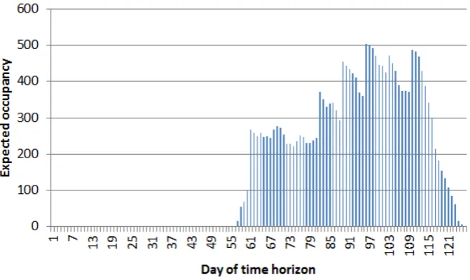
arrival day of the ascension weekend in 2014 of a certain bungalow park in the Netherlands with periods of one day.
Clearly, requests appear over time and a certain seasonality is involved here. For dierent periods in the year there is a high occupancy and periods with a low occupancy. Also, for dierent periods in the year there is a higher number of requests then other periods. Seasonality is a major factor that considerably eects the number of requests. Camping and bungalows parks usually divide their arrival horizon into dierent seasons and set prices along these seasons. Typically, a season with a high number of expected arrivals contains higher prices than a season with a low number of expected arrivals. We assume that we haveS dierent seasons during the year andSa indicates
the season in which arrival daya appears.
0 50 100 150 200 250 300 350 Days before arrival
0 20 40 60 80 100 120
Num
ber of req
uests
Figure 7: Request curve
We use B(0,a)to denote the expected number of walk-in customers at arrival day a. We assume
that reservations obey a binomial distribution with probability ρ. Thus,
B(τ,a)=Nρ
with N the size of the `potential' population of requests andρthe probability that a request will occur. We need to nd an estimate of B(τ,a) to generate future requests. However, from the
historical data we only have one realization of B(·,a). Of course, it will be inaccurate to base the
estimate of B(τ,a)on this single observation. We analyzed the historical data of several camping
and bungalow parks in the Netherlands. This data includes the date of received a request, the reservation of this request and the object type chosen by the customer of the request. From this data we observed that the shape of the request curve is quite the same within each season. As consequence, we can make our estimate more accurate by separating the eect of the request behavior B(τ,·) from the arrival process B(·,a). In particular, if we take period M as an upper bound beyond no requests occur, then we assume that
B(τ,a)=B0(τ)s(a)
with ÍM
τ=1B
0(τ)=1 and
s(a) the number of arrivals on arrival day a. Now, our goal is to nd a
good estimate Bˆ(τ,a)forB(τ,a)using
ˆ
B(τ,a)=Bˆ0(τ)ˆs(a).
When this expected number of request for each arrival day is computed, the LoS needs to be computing of each request. The LoS plays an important role, because the LoS can actually impact the occupancy. We consider a distribution of the LoS obtained from the historical data. From the data of several bungalow parks in the Netherlands we observed that the lead time does not typically impact the LoS. The major inuence factor on the LoS comes from the seasonality and day of the week (i.e. Su,Mo,..,Sa) of the arrival day a, dened by ad. Let l ∈ La, then we need
to nd the probabilities Pr(l | Sa,ad)for all S anda, which is the probability that an arrival on
arrival daya has a length of stay of l.
If the expectationsBˆ(τ,a)and probabilitiesPr(l|Sa)are known, then the request progress can be simulated over time. We developed a Monte Carlo simulator (MC-sim) which perform Bernoulli trails to nd the number of arrivals of a certain arrival day and add a LoS to each request with the corresponding probability distribution. This simulator is described in section 5.2 in more detail. Using the stochastic model we computebr,w by
br,w =Bˆ(war −w,ar) ·Pr(lr |Sar,ad). (15) Where war is the decision period for which d
1
w ≤ ar ≤ dwe and war −w denotes the number of periods before arrival daya. In the work of [21] some methods are given to nd theBˆ0(τ),ˆs(a)and
probabilitiesPr(lr|Sar,ad). In this project some easy methods are applied to nd these estimates and are only used to get an indication of the values br,w to come up with appropriate expected
5.2 Monte Carlo simulator
For purpose of simulating the request process, a binomial distribution is considered together with the expectationsB(τ,a)for allτ andaand probabilitiesPr(lr|Sar)for allr. The two quantitiesN and ρare set such that the following two equations are satised:
B(τ,a)=Nρ (16)
V ar=Nρ(1−ρ). (17)
To complete the simulation, each generated reservation needs to be provided with a length of stay. The MC-sim is build up in the following steps:
1. InitializeQ=∅.
2. Forw=w1, ...weperform the following:
(a) For alla∈ {a|dwe ≥a≥d1
w} perform the following:
IfB(τ,a),0(withτ=wa−w) then Solve (16) and (17) forNand ρwith valuesB(τ,a)
andV ar. Generate the total number of arrivals (denoted by X) for arrival daya with the binomial distribution and parameters N and ρ.
(b) If X > 0, then pick for each generated arrival a length of stay using the LoS probabilities Pr(l|Sa,ad).
(c) If X = 0, then generate an unrealized request for all reservations with arrival dayaand length of stay l∈ {l|Pr(l|Sa,ad)>0}.
(d) Randomly add the requests generated in step (2b) and (2c) toQto obtain all (realized and unrealized) request of decision period w
3. Output demand streamQ
After the Monte Carlo simulation, we end up with a demand streamQ, which is called a sample path. So, a sample path is a chronological list of requests and such a path is used as a sample path for our numerical experiments.
5.3 Maximize revenue of Monte Carlo path
In this section we proposed the computation of the maximum simulated expected revenue of a sample path. The maximum simulated expected revenue for a certain sample path is used as a benchmark in the computational experiments.
Denition 27 We deneqk
r,w as the expected number of realized (and unrealized) requests at price
class k for reservationr in decision periodw.
The valuesqrk,w are computed fromqr,w with the same demand elasticity model is used in section
3.2. Hence,
qrk,w=qr,w·DE(k) ∀k∈ K
with DE(k)the same linear price class dependent function as used for computation of the values
bkr,w. Moreover, if qr,w =0 andbr,w >0, then we use the extended demand elasticity function as
described in section 4.2.2 to computeqrk,w. The maximum simulated expected revenue of a sample path is found by solving the AER-ILP with values qrk,w instead of the values bkr,w and is found in ILP (18) - (21). The output variables ˆvrk,w denotes the optimal dynamic pricing strategy for
sample pathQ. ILP (18) - (21) is called the optimal aggregated simulated expected reservation ILP (OPT-ILP) and the maximum simulated expected revenue and pricing strategyˆvrk,w is found by
solving
max Õ
w∈ D
Õ
r∈ R ar≥dw1
Õ
k∈K
vrk,wprkqrk,w (18)
s.t. Õ
w∈ D
Õ
r∈ R ar≥dw1
Õ
k∈K
ai,rvrk,wqrk,w ≤ci ∀i∈ I (19)
Õ
k∈K
vrk,w=1 ∀r∈ R,∀w∈ D (20)
vkr,w ∈ {0,1} ∀r∈ R,∀k∈ K,∀w∈ D. (21)