University of Warwick institutional repository: http://go.warwick.ac.uk/wrap
This paper is made available online in accordance with
publisher policies. Please scroll down to view the document
itself. Please refer to the repository record for this item and our
policy information available from the repository home page for
further information.
To see the final version of this paper please visit the publisher’s website.
Access to the published version may require a subscription.
Author(s): Robin C. Ball, Thomas M. A. Fink and Neill E. Bowler
Article Title: Stochastic Annealing
Year of publication: 2003
Link to published article:
http://dx.doi.org/10.1103/PhysRevLett.91.030201
arXiv:cond-mat/0301179v1 [cond-mat.stat-mech] 13 Jan 2003
Robin C. Ball,1,∗ Thomas M. A. Fink,2, 3,† and Neill E. Bowler1,‡
1
Department of Physics, University of Warwick, Coventry CV4 7AL, England 2
CNRS UMR 144, Institut Curie, 75005 Paris, France 3
Theory of Condensed Matter, Cavendish Laboratory, Cambridge CB3 0HE, England
(Dated: February 2, 2008)
We demonstrate that is it possible to simulate a system in thermal equilibrium even when the energy cannot be evaluated exactly, provided the error distribution is known. This leads to an effective optimisation strategy for problems where the evaluation of each design can only be sampled statistically.
PACS numbers: 02.60.Pn, 05.10.Ln, 02.50.Ng
Keywords: stochastic optimisation, simulated annealing
We consider thermal equilibrium simulation of systems in which the energy of any given state is either not known exactly, or else can much more cheaply be estimated. A classic example which occurs in Physics is where each en-ergy calculation itself involves sampling over a distribu-tion or numerical integradistribu-tion, or the estimadistribu-tion of param-eters of a numerical model. In this letter we show how, by Stochastic Annealing, thermal equilibrium distribu-tions can nevertheless be sampled exactly, the essence of our method being that the energy errors can be precisely absorbed as a contribution to thermal noise.
Our thermal sampling technique can be applied to opti-misation problems where the objective function is analo-gously difficult to evaluate, using Simulated Annealing[1] (meaning simulated cooling) or related methods [2, 3]. As an example we consider designing model protein molecules to fold as fast as possible, where the only way to evaluate a particular design is to run a sample of folding simulations. Confronted by similar problems others have developed more empirical methods [4, 5, 6], but none of these is underpinned by simulation of true thermal equilibrium.
In a thermal ensemble the probability of the system occupying a stateµwith energyE(µ) is
P(µ)∝e−βE(µ) (1) where β = T1 is the inverse temperature. It is conve-nient to sample this distribution by a Markov process, in which the system is allowed to make a transition (move) from one state to another with rate constantK(µ→ν) which depends only on the two states concerned. This is generally more efficient than trying to choose the states directly, provided we can assume that the move set is ergodic, meaning that all states can be reached (even-tually) from any given starting state. The more strict condition of detailed balance,
P(µ)K(µ→ν) =P(ν)K(ν →µ), (2)
imposes the correct equilibrium distribution provided K(µ→ν)
K(ν→µ) =e
−β∆E (3)
where ∆E is the energy differenceE(ν)−E(µ).
Whilst eq. (3) ensures thermal equilibrium at inverse temperature β, it does not fully determine the form of K. Typically K(µ → ν) is the combination of an at-tempt frequency to move to stateν given that the system is in state µ, multiplied by an acceptance probability. For simplicity of exposition we will take all the attempt frequencies to be equal to unity, so that K is just an acceptance probability and so must obey 0 ≤ K ≤ 1. The Metropolis algorithm[7] is fully specified by requir-ing thatK(∆E) = 1 for ∆E < C, with C as large as possible (maximising acceptance rates) leading to
KMetropolis(∆E) = min 1, e−β∆E
, (4)
whereas the Glauber acceptance function [8] arises by requiring thatK(∆E) +K(−∆E) = 1, leading to
KGlauber(∆E) = 1/ 1 +eβ∆E
. (5)
These are compared graphically in Fig. 1.
We now consider the case when the true energy change is not known exactly, and we must accept moves with probabiltyA(x) where xis only an estimate of the en-ergy change. We will assume that these estimates have statistically independent errors. Iff(x|∆E) is the prob-ability density of estimating that the energy change is xwhen its true value is ∆E, then the net probability of accepting a move whose true energy change is ∆E is given by
K(∆E) =
Z ∞
−∞
f(x|∆E)A(x)dx. (6)
It is our aim to chooseA(x) such that K(∆E) satisfies detailed balance (3).
2
x AHxL
x- DE fHx - DEL
*
DE þþþþþþþþþþþ T K@DED
[image:3.612.67.275.51.219.2]Metropolis Glauber convolution
FIG. 1: A simple approximate stochastic annealing is ob-tained by accepting moves on the basis of the sign of the estimated energy change x. The acceptance probability as a function of the true underlying energy change ∆E is then given by a convolution with the error distribution. As shown for the Gaussian distribution case, this gives an excellent approximation to the exact Glauber acceptance rule.
acceptance function (whose symmetry it shares) is strik-ing, showing how the random energy errors make the selection look thermal - although in this case the match is not exact, so detailed balance is not strictly achieved. The standard deviation σ of the Gaussian distribution controls an approximate effective temperature using this rule, as inverting eq. (3) gives
T ≃ r
π 8σ
1−0.018 (∆E/T)2+ order (∆E/T)4. (7)
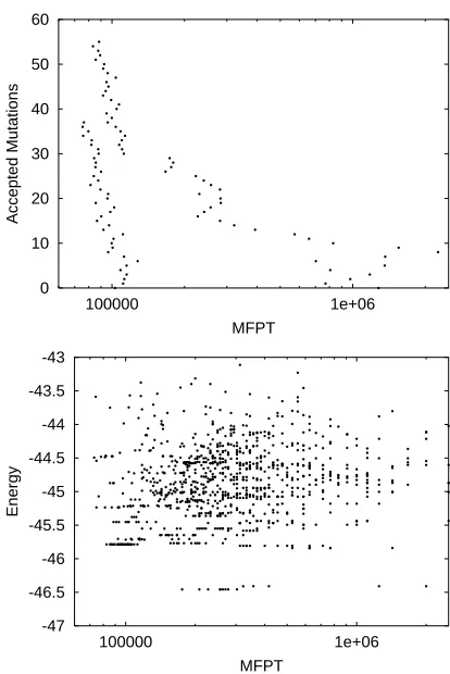
For many optimisation purposes the departure from de-tailed balance, due to the energy dependent terms at large|∆E/T|, is not a problem. Fig. 2 shows how we successfully used this approach to optimise model protein folding: for each design change considered we obtained estimates of the change in mean folding time from a lim-ited sample of folding simulations, and as the annealing proceeded we gradually cooled the system by increasing the sample sizes leading to reduced error size and re-duced temperatures through Eq 7. In another paper[9] we show that this approach can be exploited to unravel a benchmark problem in stochastic optimisation, the prob-abilistic travelling salesman problem [10, 11].
We now attempt directly to chooseA(x) properly, such thatKexactly satisfies detailed balance, eq. 3, assuming that the error distribution f(x|∆E) is fully known. We first note that this leads to some bounds on the behaviour of the right tail ofA(x) and a left tail off(x|∆E).
Given that K(∆E) ≤ 1 even for negative argu-ments, the detailed balance condition requiresR−∞∞ f(x| ∆E)A(x)dx ≤ e−β∆E and for large positive ∆E this
severely restricts all contributions to the LHS. First
con-0 10 20 30 40 50 60
100000 1e+06
Accepted Mutations
MFPT
-47 -46.5 -46 -45.5 -45 -44.5 -44 -43.5 -43
100000 1e+06
Energy
MFPT
FIG. 2: Stochastic annealing applied to protein folding, in a simple cubic lattice model. The chains were 27 units long and the space of amino acid sequences was explored for the ability of the molecule to fold spontaneously to a fixed 3×3×3 cubic target conformation. (a) The upper panel shows the result of two stochastic annealing simulations in which successive mutations of a starting sequence were accepted if a limited sampling of the Mean First Passage Time (to the target) was improved. Increasing the depth of sampling as the anneal-ing proceeded (y-axis) provided the analogue of lowering the temperature. (b) For comparison the lower panel shows the result of an extensive search over sequences guided by thermal stability (energy in the target conformation). Clearly indi-vidiual runs of Stochastic Annealing find folding speeds ap-proaching the fastest available, and much better than would be achieved by seeking minimum energy (the Shaknovitich scheme [12]).
siderx≃∆E for whichf(x|∆E) is not expected to be small. Then the exponential decay on this contribution must come fromA(x) falling off at least as fast ase−βxas
x→ ∞, which becomes important in our later analysis. Second considerx.0, for which A(x) cannot become small or we would be heavily rejecting even moves which appear to be downwards in energy. Then the exponen-tial decay on this contribution must come fromf(x|∆E), x.0, falling off at least as fast ase−β∆E for ∆E→ ∞.
[image:3.612.331.538.52.362.2]thermal Boltzmann factor.
Now we begin direct analysis of the detailed balance condition (3), inroducing the substitutions f(x|∆E) = eβ2(x−∆E)g(x,∆E) andA(x) =e−
βx
2 a(x) so that eqs. (3) and (6) combined simplify down to
Z ∞
−∞
a(x) (g(x,∆E)−g(x,−∆E))dx= 0. (8)
Without significant loss of generality we can try
a(x) =
Z ∞
−∞
h(∆E′)j(x,∆E′)d∆E′ (9)
where hand j are functions to be chosen. Substituting this into equation 8 we find
Z ∞
−∞
h(∆E′) [k(∆E,∆E′)−k(−∆E,∆E′)]d∆E′ = 0
(10) where
k(∆E,∆E′) =
Z ∞
−∞
g(x,∆E)j(x,∆E′)dx. (11)
Then eq. 10 is satisfied when h(∆E′) = h(−∆E′) and k(∆E,∆E′) =k(−∆E,−∆E′) are even functions in the given sense. We have not succeeded in taking this most general case significantly further, the hard part being to implement 0≤A(x)≤1 for a probability.
For further progress we now specialise to the case of in-variant error distributions, wheref(x|∆E) =f(x−∆E), meaning that the distribution of error is independent of ∆E itself. For this case, we can choose j(x,∆E′) = g(x−∆E′) and then from eq. 11 we findk(∆E,∆E′) is
a suitably even function. Then we have a solution to eq 8 given by
a(x) =
Z ∞
−∞
h(∆E′)g(x−∆E′)d∆E′ (12)
providedh(x), and correspondinglyeh(p) below, is even. We now aim to choosehto maximise the move accep-tance rates, which are governed byA(x). We follow the Metropolis methodology in choosingA(x) (=e−βx
2 a(x)) to be identically 1 below some threshold, x < C. Then using the Fourier-Laplace transform defined by fe(p) =
R∞
−∞e
−pxf(x)dx,the transform ofabecomes
ea(p) =
Z C
−∞
eβx2 e−pxdx+
Z ∞
C
b(x)e−pxdx (13)
where b(x) = A(x)eβx2 for x≥ C, b(x) = 0 for x < C. From eq.(12) the transform of the new function b(x) is given by
eb(p) =eh(p)eg(p)−e (β
2−p)C
β
2 −p
. (14)
The exponential bound we established on the right tail ofA(x) implies thateb(p) is bounded for all Rep >−β2,
whereas the integrability of f(x) together with the ex-ponential bound on its left tail only imply that eg(p) is bounded for−β2 ≤Rep <
β
2. Thuseh(p) must be
cho-sen to cancel both any divergences ofge(p) in Rep≥ β2
and the apparent pole atp=β/2. We first turn to the Wiener-Hopf method [13] to define
e
g(p) =gfL(p)gfR(p) (15)
wheregfL(p) is bounded and non-zero for Rep < β2, and
f
gR(p) is bounded and non-zero for Rep > β2 ; it also
follows from the bounded window for eg(p) that gfR(p)
is bounded for the wider range Rep > −β2. Then
by choosingeh(p) = ((β/2)B2−p2)
1
f
gL(p)gfL(−p) , we can
en-sure thateh(p)eg(p) = ((β/2)B2−p2) f
gR(p)
f
gL(−p) is duly bounded
for Rep > −β2 except for the (desired) pole at p =
β
2.
Choosing the constantB =βfgL(−β2)
f
gR(β2) makes the residue
of this pole cancel when we reassemble the expression (14) foreb(p) to give
eb(p) =−e(
β
2−p)C
β
2 −p
+ β
(β/2)2−p2 f gR(p)gfL
−β2
f gR β 2 f gL(−p)
.
(16) This should be the optimal solution. We cannot in-corporate any new factors intoeh(p) because, being even, they would have to be bounded both for Re(p) > −β2
and for Re(p) > β2, and we would run up against the limitations of Liouville’s Theorem. The parameter C might appear to be a remaining degree of freedom, but it drops out of the acceptance function itself which is given directly in terms of
ea(p) =eh(p)eg(p) = β (β/2)2−p2
f gR(p)gfL
−β2
f gR β 2 f gL(−p)
. (17)
The parameterCdrops out because it simply reflects the partition we introduced in equation (13). The feature which we have not strictly guaranteed is thatA(x) = 1 forx < C rather than some different cutoff.
As an example of our approach above, consider the simple case where
f(x−∆E) = γ 2e
−γ|x−∆E| (18)
which leads to eg(p;γ) = ( γ2
γ−β
2−p)(γ+
β
2+p)
. The choice
of fgL and gfR is trivial by inspection, giving ea(p) = β
(β/2)2−p2
γ+β
γ
γ−β2+p
γ+β
2+p
.The inverse transformation can also be performed by inspection to give
A(x) = min
1,γ 2−β2
γ2 e
−βx+β2
γ2e −(γ+β)x
4
We note that this acceptance function only remains pos-itive for x ≫ 0 when γ ≥ β, which is precisely the limit of achievable stochastic annealing discussed earlier, and the case γ → ∞ also duly recovers the straightfor-ward Metropolis method. We have analysed other simple cases such as a rectangular error distribution, the super-position of two exponentials as above, and the multi-ple convolution of exponentials, all leading to results of equivalent properties.
The analysis of a Gaussian error distribution turns out to be slightly singular, in that its corresponding eg(p) has no obvious Wiener-Hopf factorisation. However we can approach it by considering the case wherexis taken to be a sum of N independent exponential-distributed variables, the error distribution taking the solvable form of multiply convolved exponentials and (by the Central Limit Theorem) approaching Gaussian form asN→ ∞. In this case eg(p) = eg(p;γ)N with γ = √2N/σ, where
σ is the standard deviation of x, leading to ea(p) =
β
(β/2)2−p2
γ+β
γ
γ−β2+p
γ+β
2+p
N
→ (β/2)β2−p2e
β(p−β/2)σ2/2
as N → ∞at fixedσ. The corresponding acceptance func-tion by inverse transformafunc-tion is then given by
A(x) = min1, e−β(x+βσ2/2) (20) The optimal acceptance rules found above all obey the bounds that 0 ≤ A(x) ≤ 1 required for a proba-bility, but they only do so a postiori so it can be ob-jected that our optimal method gives no guarrantee of this outcomea priori. We have discovered a general but sub-optimal solution for the acceptance function which does assure the requirement. The key to this solution is to note that, given the result 17, our requirements on the factorisation of eg(p) can be relaxed to require only that gfR(p) is bounded for Rep > −β2 and that
f
gL(p) is non-zero for Rep < β2. Then assuming that
f(x) = 0 forx < C, an acceptable factorisation is given by gfR(p) = eg(p)epC, gfL(p) = e−pC leading directly to
e
a(p) = eh(p)eg(p) = ( β
(β/2)2−p2) e
g(p)
e
g(β2), at which point we
can let C → −∞ so no significant new restriction has been imposed on f. The resulting acceptance function by inverse transformation can be expressed as the convo-lution
A(x) = 1 e f(β)
Z ∞
−∞
KMetropolis(x−y)e−βyf(y)dy. (21)
It can be verified by direct substitution that this does obey the detailed balance condition (3), it is manifestly positive definite, and it gives maximum acceptance 1 as x → −∞. Simple comparison shows the resulting ac-ceptance probabilities are lower than the optimal values which we have calculated these, and the key difference is that an interval whereA= 1 is no longer imposed.
Given the wide impact of equilibrium statistical me-chanics, we are confident that our new method of exactly
thermal stochastic annealing will find significant direct application. The chief limitation is that the error distri-bution must be known. In this context the Gaussian case is particulary important as it can be approached simply through multiple sampling, although its variance is also required. Estimating the variance from the same sample does induce errors, but these can be quantified and be-come negligible as the sample size bebe-comes large[14]. It is a more open question whether it is viable to estimate by measurement the full distribution of error and apply this to eq. (21).
Underpinned by the exact results our analysis provides a powerful new tool in stochastic optimisation. Gener-ally it will be sufficient and convenient to use the approx-imately thermal method we presented, of simply accept-ing moves which appear to be an improvement. Then all the benefits of simulated annealing are obtained by delib-erately using crude estimates for each decision! In the protein folding problem we used limited samples of fold-ing time for these estimates, makfold-ing the high tempera-ture part of the annealing computationally the cheapest. This interestingly complicates the long noted problem of how to choose the optimum cooling schedule, because cooling by reducing sample errors introduces computa-tional costs growing as 1/T2per move.
NEB would like to thank BP and EPSRC for the sup-port of a CASE award during this research.
∗ Electronic address: [email protected];
URL:http://www.phys.warwick.ac.uk/theory/ † Electronic address: [email protected];
URL:http://www.tcm.phy.cam.ac.uk/~tmf20/ ‡ Electronic address: [email protected];
URL: http://uk.geocities.com/neill_bowler;
Present address: Met Office, Maclean Building, Crowmarsh-Gifford, Oxfordshire OX10 8BB, UK. [1] S. Kirkpatrick, C. D. Gelatt Jr and M. P. Vecchi,Science
220, 671 (1983).
[2] A. Harjuet al.,Phys. Rev. Lett.79, 1173 (1997). [3] Edward J. Anderson and Michael C. Ferris,SIAM J.
Op-timiz.11, 837 (2001).
[4] H. Robbins and S. Munro, The annals of mathematical statistics22, 400 (1951).
[5] W. B. Gong, Y. C. Ho, and W. Zhai, in Proceedings of the 31st IEEE conference on decision and control(IEEE, PO Box 1331, Piscataway, NJ, 1992), pp. 795–802. [6] A. A. Bulgak and J. L. Sanders, in Proceedings of the
1988 Winter Simulation Conference (IEEE, PO Box 1331, Piscataway, NJ, 1988), pp. 684–690.
[7] N. Metropolis, A. W. Rosenbluth, M. N. Rosenbluth, A. H. Teller, and E. Teller, J. Chem. Phys. 21, 1087 (1953).
[8] R. J. Glauber, J. Chem Phys4, 294 (1963).
[9] N. E. Bowler, T. M. Fink, and R. C. Ball, Characteri-zation of the probabilistic travelling salesman problem, submitted to Physical Review E.
[11] P. Jaillet,Math. Oper. Res.18, 51 (1993).
[12] A. M. Gutin, V. I. Abkevich and E. I. Shakhnovich,Proc. Natl. Acad. Sci. USA92, 1282 (1995).
[13] P. M. Morse and H. Feshbach, inMethods of theoretical
physics(McGraw-Hill, London, 1953), pp. 978–980. [14] N.E. Bowler, PhD Thesis, University of Warwick, UK