Optimization of transmitted reference receivers in the ultra wide bandwidth system

(1)

University of Warwick institutional repository: http://go.warwick.ac.uk/wrap

A Thesis Submitted for the Degree of PhD at the University of Warwick

http://go.warwick.ac.uk/wrap/45884

This thesis is made available online and is protected by original copyright. Please scroll down to view the document itself.

(2)

AUTHOR:Shuyi Wang DEGREE:Ph.D.

TITLE: Optimization of Transmitted-Reference receivers in the Ultra-wide Bandwidth System

DATE OF DEPOSIT: . . . .

I agree that this thesis shall be available in accordance with the regulations governing the University of Warwick theses.

I agree that the summary of this thesis may be submitted for publication. Iagreethat the thesis may be photocopied (single copies for study purposes only).

Theses with no restriction on photocopying will also be made available to the British Library for microfilming. The British Library may supply copies to individuals or libraries. subject to a statement from them that the copy is supplied for non-publishing purposes. All copies supplied by the British Library will carry the following statement:

“Attention is drawn to the fact that the copyright of this thesis rests with its author. This copy of the thesis has been supplied on the condition that anyone who consults it is understood to recognise that its copyright rests with its author and that no quotation from the thesis and no information derived from it may be published without the author’s written consent.”

AUTHOR’S SIGNATURE: . . . .

USER’S DECLARATION

1. I undertake not to quote or make use of any information from this thesis without making acknowledgement to the author.

2. I further undertake to allow no-one else to use this thesis while it is in my care.

DATE SIGNATURE ADDRESS

. . . .

(3)

M A E

G NS

I T A T MOLEM

U N

IV

ER

SITA_{S WARW}ICE

NS

IS

Optimization of

Transmitted-Reference receivers in

the Ultra-wide Bandwidth System

by

Shuyi Wang

Thesis

Submitted to the University of Warwick

for the degree of

Doctor of Philosophy

School of Engineering

(4)

List of Figures

1.1 The definition of UWB systems. . . 4

1.2 The FCC UWB spectral masks. . . 5

2.1 The realizations of the channel impulse response for different

scenarios (CM1-CM4). . . 18

2.2 The Gaussian doublet in the time domain defined in (2.9). . . 20

2.3 The Gaussian doublet in the frequency domain defined in (2.12). 21

2.4 Comparison of several different modulation techniques for UWB

communications:(a) unmodulated pulses, (b) BPPM and (c)

PAM. . . 23

2.5 A typical structure of the UWB TH-SS system with two users. 26

2.6 A typical structure of the UWB DS- system with three users. . 28

3.1 The system model of the conventional TR receiver with different

values of Td. . . 40

3.2 The channel achievable capacity versus Td for the traditional

TR receiver by using the simulation method. . . 46

3.3 The channel achievable capacity versus Td for the traditional

(8)

3.4 The channel achievable capacity versus Tdby using simulation,

semi-analytical and analytical methods. . . 59

3.5 The channel achievable capacity versus SNR for the traditional

and improved TR receivers for CM1. . . 62

3.6 The channel achievable capacity versus Tdby using simulation,

semi-analytical and analytical methods for CM2. . . 63

3.7 The channel achievable capacity versus SNR for the traditional

and improved TR receivers for CM2. . . 64

3.8 The BER versus Td for the traditional TR receiver at different

SNRs for CM1. . . 68

3.9 The BER versus SNR for the traditional and improved TR

re-ceivers for CM1. . . 69

4.1 The BER versus α for the generalized TB receiver at TN =Tds

for different SNR scenarios. . . 80

4.2 The BER versus α for the generalized ML-I receivers at TN =

Tds for different SNR scenarios. . . 81

4.3 The BER versusαfor the generalized GLRT-I receivers atTN =

Tds for different SNR scenarios. . . 81

4.4 The BER versus SNR at the optimal α for the generalized TB

and ML-I receivers. . . 83

4.5 The BER versus SNR at the optimal α for the generalized

GLRT-I receivers. . . 83

4.6 The BER versus TN at the optimum values ofα for the

(9)

gener-alized ML-I receivers. . . 85

gener-alized GLRT-I receivers. . . 85

4.9 The BER versus SNR atTN opt, αopt andαopt for the generalized

TB and ML-I receivers. . . 87

4.10 The BER versus SNR at bothα and TN optimized for the

gen-eralized GLRT-I receivers. . . 87

4.11 Comparison of the improved TB and ML-I receivers that

op-timize α first and the improved TB and ML-I receivers that

optimize TN first. . . 88

4.12 Comparison of the improved GLRT-I receivers that optimize α

first and the improved GLRT-I receivers that optimize TN first. 89

4.13 The BER versus SNR atTN opt, αopt andαopt for the generalized

ML-II and GLRT-II receivers. . . 90

4.14 Comparison of the improved ML-II and GLRT-II receivers that

optimize α first and those that optimizeTN first. . . 91

4.15 The BER versusα at SNR = 10 dB and TN =Tmds. . . 99

4.16 The BER versus SNR for non-improved receivers and improved

receivers using αopt. . . 100

4.17 The BER versusTN using αopt at SNR = 10 dB. . . 101

4.18 The BER versus SNR using neither αopt or TNopt,αopt and both

αopt and TNopt,αopt. . . 104

4.19 Comparison of the simulated improved receivers that optimize

α first and the simulated improved receivers that optimize TN

(10)

List of Tables

3.1 The Best Values of Td (ns) for Different SNRs. . . 66

4.1 The Best Values of α and TN(ns) for the Simulated TR

(11)

Acknowledgments

I would like to acknowledge the advice and guidance of my supervisors, Dr.

Yunfei Chen and Dr. Mark S. Leeson from the School of Engineering at the

University of Warwick. I also thank the members of my graduate committee

for their suggestions and encouragement, especially Prof. Roger J. Green.

Special thanks go to Prof. Norman C. Beaulieu from the University of

Alberta Edmonton, Canada, for his knowledge and assistance in this studies.

I would like to thank my family members, especially my mother, Ms

Yawei Niu, for her supporting and encouraging me to pursue this degree. Last

but not least, I express my sincere appreciation to all my friends who have

(12)

Declarations

I herewith declare that I have produced this paper without the prohibited

assistance of third parties and without making use of aids other than those

specified; notions taken over directly or indirectly from other sources have been

identified as such. This paper has not previously been presented in identical

or similar form to any other examination board.

The thesis work was conducted from April 2008 to June 2011 under the

(13)

List of Publications

Journal Papers

• Shuyi Wang, Yunfei Chen, Mark S. Leeson, Norman C. Beaulieu,

“Channel Capacity and BER Optimization of the UWB Dual-Pulse

Re-ceiver”,Wireless Communications and Mobile Computing, doi: 10.1002/

wcm.1214, November 2011.

• Shuyi Wang, Yunfei Chen, M. Leeson, N.C. Beaulieu, “New receivers

for generalized UWB transmitted reference systems with improved

per-formances”,IEEE Transactions on Wireless Communications, vol.9, no.6,

pp.1837-1842, June 2010.

• Yunfei Chen, N. Beaulieu; Shuyi Wang, “Novel iterative receivers for

TR UWB systems”,IEEE Communications Letters, vol.13, no.4,

pp.242-244, April 2009.

Conference Papers

• Shuyi Wang, Yunfei Chen, Mark S. Leeson, Norman C. Beaulieu,

“Optimization of the Time Delay in the UWB Dual-pulse Receiver”,

2011 IEEE International Conference on Ultra-Wideband, pp. 445-449,

(14)

Abstract

This thesis contributes the research and development of novel receiver

optimization approaches conducted in ultra-wide bandwidth (UWB) systems.

The ultimate goal of the improved receiver technology is to simplify the receiver

structures at the cost of a tolerable performance degradation or improve the

receiver performances at the cost of a tolerable complexity. Recently, UWB

technology has become more and more attractive due to its increased

per-formance. An advanced scheme that can provide a further improvement is

strongly recommended and highly demanded. This research project focuses

on the design of outstanding receivers suitable for the UWB system with

transmitted-reference signaling. Two types of improved receivers are

inves-tigated. The first one is based on the optimization of inter-pulse time delayTd

in the traditional transmitted-reference receivers where one data pulse is

trans-mitted Td seconds delay after one reference pulse in a bit duration. The

sec-ond one is based on the joint optimization of the number of reference symbols

and the integration interval length in the generalized transmitted-reference

receivers where Nd data symbols are transmitted after Nr reference symbols

in a data packet. For both improved receivers, simulation and theoretical

ap-proaches are used to provide the optimization results. The numerical results

show that the improved receivers by using different optimization approaches

(15)

An up to 4.2dB performance improvement can be achieved consequently.

The principal conclusion from this thesis is that all the optimization

schemes presented herein can be successfully applied to the design of receivers

in the UWB transmitted-reference systems that the data decision can be

ob-tained by thresholding the correlator output of the reference information with

(16)

Abbreviations

UWB descriptive ultra-wide bandwidth

TR descriptive transmitted-reference

WPAN descriptive wireless personal area network

LLNL descriptive Lawrence Livermore national laboratory

DoD descriptive department of defense

FCC descriptive Federal communications commission

Ofcom descriptive office of communications

MIC descriptive ministry of internal affairs and communications

EIRP descriptive equivalent isotropically radiated power

GPS descriptive global positioning system

LPD descriptive low probability of detection

LPI descriptive low probability of interception

SNR descriptive signal-to-noise ratio

MAI descriptive multiple access interference

(17)

BER descriptive bit error rate

S-V descriptive Saleh-Valenzuela

LOS descriptive line-of-sight

NLOS descriptive non line-of-sight

PDF descriptive probability density function

PSD descriptive power spectral density

PPM descriptive pulse position modulation

PAM descriptive pulse amplitude modulation

OOK descriptive on-off keying

BPPM descriptive binary pulse position modulation

BPAM descriptive binary pulse amplitude modulation

TH descriptive time-hopping

SS descriptive spreading spectrum

DS descriptive direct-sequence

PN descriptive pseudo-noise

AWGN descriptive added white Gaussian noise

(18)

Chapter 1 Introduction

1.1 Introduction to Ultra-wide Bandwidth

Sys-tems

Over the last couple of decades, consumers’ demands for wireless technologies

have been dramatically increased due to the enormous convenience brought

by modern technologies to the real-life world. In the near future, consumers

will continuously increase their requirements for wireless connectivities to

con-nect electronic devices, such as personal computers, portable game systems,

mobile phones, photo printers and radio/video players, to each other in the

home. However, today’s short- or medium-range wireless communication

tech-nologies cannot meet the needs of such high compatibility which require very

wide bandwidth, accommodating the needs for high capacity and data rate.

For example, although the data rate can reach up to 54 Mbits per second for

the IEEE 802.11 standards, the technologies have limitations in bandwidth,

(19)

technol-ogy (belongs to IEEE 802.15.1) trades its cost and power consumption off the

data rate of up to 1 Mbit per second [2] which is not sufficient for many

mul-tiple high-bandwidth digital applications in wireless personal area networks

(WPANs). A novel technology named ultra-wide bandwidth (UWB) was

in-vestigated accounting for the high-speed WPANs [3].

1.1.1 Historical development of UWB Technologies

In the long history of radio communications, the dominant electromagnetic

waveform was sinusoidal. The sine-wave was so universal until the

develop-ment of the sampling oscilloscope dating back to the early 1960s. The

de-velopment of hardware devices attracted many institutes and companies to

embark on the pulse transmitter, receiver and antenna investigations. In the

1960s, Lawrence Livermore National Laboratory (LLNL) was one of the

pio-neers leading the research in this area and many applications and technologies

were then imported to UWB communications [4].

By the early 1970s the foundation of UWB radar systems were almost

accomplished [4] and especially in 1973, Ross’ US Patent [5] indicated that

the comprehensive development of UWB systems had entirely started.

Inter-ested readers can refer to [4], [5] and [6] for further pioneer works for UWB

all over the world. At the early stage, the UWB technologies were using

base-band, carrier-less, impulse and time domain. The term ‘ultra-wide

band-width (UWB)’ was first determined by the US Department of Defense (DoD)

in 1989, since it occupies an extremely wide bandwidth. In the last century,

UWB technologies have been diffusely used in numerous fields, such as

(20)

few applications developed for data communications like PC- or mobile-device

communications [7].

In April 2002, the US Federal Communications Commission (FCC)

re-leased its report [8], first indicating that UWB technologies could be used

in data communications as well. In [8], it defined UWB communication

sys-tems from many aspects, including UWB definition, bandwidth allocation and

maximum transmission power. These FCC regulations have been widely

ac-cepted and applied for UWB systems, although some countries have their own

variations. For example, the regulator in the UK is the Office of

Communi-cations (Ofcom) and the regulator in Japan is the Ministry of Internal Affairs

and Communications (MIC), and they released their own standards for UWB

communication systems in 2005 and 2004, respectively. However, the

differ-ences in UWB standards among various countries are not significant [9].

Interested readers can refer to [10], [11] and [12] for further historical

reviews of UWB technologies.

1.1.2 FCC Regulations for UWB

The UWB system was defined by FCC [8] in 2002 as a transmission system

with a bandwidth occupancy of more than 500 MHz or the fractional

band-width greater than 20%, as shown in Figure 1.1, where fL and fH represent

the lower and upper frequencies, respectively, at the -10 dB emission point.

Also,fc = fL+₂fH represents the centre frequency. The fractional bandwidth is

determined by B_f_c, where B =fH −fL is the -10 dB bandwidth (10 dB below

the highest emission point). According to [8], the newest UWB system either

(21)

[image:21.595.161.471.111.290.2]

Figure 1.1: The definition of UWB systems [8].

bandwidth greater than 20% when fc <2.5 GHz.

The FCC allocated specific ranges of GHz bandwidth to UWB

commu-nication systems [8]. This extremely wide bandwidth allows UWB systems to

potentially have a high data rate on the order of Gbps (Gbits per second). On

the other hand, UWB has to coexist with other narrowband and wideband

communication systems over the entire frequency bands. Therefore, the FCC

limited the maximum transmission power such that UWB could not conflict

with other existed systems.

Figure 1.2 shows the UWB spectral masks based on FCC 15.517 for

indoor communications. The Equivalent Isotropically Radiated Power (EIRP)

denotes the theoretical power from an isotropic antenna to produce the peak

power in the direction of maximum antenna gain, taking into account the

attenuations during transmission and from devices like an antenna. A

conser-vative maximum emission power spectral density of -41.3 dBm/MHz is allowed

approximately over the total 7.5 GHz bandwidth between 3.1 and 10.6 GHz,

(22)

[image:22.595.169.468.112.284.2]

Figure 1.2: The FCC UWB spectral masks [8].

-75.3 dBm/MHz due to the existence of the global positioning systems (GPS)

and some military applications.

For further detailed FCC UWB regulations, interested readers can refer

to [8] or via the FCC official website ‘http://www.fcc.gov/’.

1.1.3 Characteristics of UWB

The UWB techniques have attracted great interest from both research and

industry, because of some of the inherent features which make UWB optimal

for low-cost, high-speed WPANs. The key benefits of UWB are listed as below:

• high data rate;

• low complexity and low cost;

• low probability of detection (LPD) and low probability of interception(LPI);

• increased capacity;

(23)

A potential data rate in the order of Gbps can be achieved in UWB,

owing to its extremely high spectral occupancy [13]. From a commercial point

of view, the high data rate is the vital factor in today’s manufacture for new

digital applications. The UWB technologies will bring a new generation of

personal wireless communications.

Unlike conventional communication systems, the UWB system

gener-ates a series of very short time-domain pulses which do not need sine-wave

car-riers to propagate. Consequently, the UWB system can be considered as

com-parably easy implementation and with low cost because no additional product

is required at transmitters or receivers.

According to the UWB spectral masks shown in Figure 1.2, the UWB

signal is substantially noise-like due to its low power density. This makes the

signal quite difficult for unintended detection and also significantly reduces

the interference between the UWB system and other existing systems. This

property benefits UWB for secure and military applications [14].

Based on Shannon’s theory, the channel capacity in an additive white

Gaussian noise (AWGN) channel is expressed as [13]

C =Blog(1 + S

N) (1.1)

where B is the channel bandwidth as described in section 1.1.2, and S

N is

the signal-to-noise ratio (SNR) of the channel. Clearly, the achievable

chan-nel capacity grows linearly with bandwidth but logarithmically with SNR and

therefore, the bandwidth B is the dominant factor affecting the channel

ca-pacity. The UWB system thereby has a potential of relatively high channel

(24)

Finally, UWB is commonly known as a low-power and short-range

wire-less communication system whose efficient transmission distance is normally

less than 20 meters. That dramatically increases the system frequency reuse

capability, as the users in different clusters can use the same frequency without

interference. For example, player one (in a cluster) who is playing a wireless

game (like WII) in the living room would not disturb the person (in another

cluster) who is printing photos via a wireless printer in the study room, when

they are using the same frequency bands.

1.1.4 UWB Applications

The UWB signal contains abundant low frequency components such that it

enables the system to be capable of penetration and hence, the UWB

technolo-gies can be applied to imaging systems, such as wall radar imaging, medical

imaging and surveillance systems [16].

Furthermore, owing to the fine time resolution and accurate position

capabilities, UWB technologies can be applied for vehicular radar systems [17].

Consequently, they can be used to improve automotive safety and provide

excellent services, such as safer airbag development and parking assistance.

For wireless communications, UWB enables a wide range of applications

in WPANs. UWB wireless speaker/mouse/USB and even completely freeing

cables among portable devices in the home can be realized, for example.

Sim-ilarly, UWB technologies can also be applied in wireless sensor networks, due

(25)

1.1.5 Challenges for UWB

In spite of the numerous advantages of the UWB technology which make it

have an optimistic future for the next generation of communications, many

problems still need to be resolved for UWB to become a widely adopted

tech-nology [19].

A main problem that has always been of concern in UWB is about the

cancellation of multiple access interference (MAI) and narrowband interference

(NBI). Precise synchronization to the extremely short pulse, accurate channel

estimation of the dense multipath coefficients, and adaptive receiver designs

are also some of the key challenges that still have to be improved.

Other challenges include precise channel models in various

environ-ments, high-speed data sampling devices, appropriate multiple access and

mul-tiple access code designs, as well as compatible and universal standard/protocol

solutions outside the physical layer.

1.2 Research Objective

Although UWB technology can be applied for data communications as well as

radar and safety applications, this thesis focuses on investigations of UWB for

data communications.

For the UWB wireless communications, receiver design is a crucial link

to a successful implementation of the entire system. In an indoor environment,

there exists a dense multipath propagation due to a great number of

obsta-cles in the building. In order to take full advantage of these rich multipath

components, an appropriate receiver is required to capture as much energy

(26)

efficient power-collection receiver with a relatively simple structure is highly

desire. The current UWB receivers can be classified into two types: coherent

receivers and non-coherent receivers. The transmitted-reference (TR) receiver

is the most common UWB non-coherent receiver in the literature, and it can

be further categorized into, for example, the traditional TR receiver or

gener-alized TR receiver. The performances of all these receivers can be improved by

either optimizing the time interval between the reference and data pulse per

bit for traditional TR receivers or optimizing the number of reference

sym-bols as well as the integration interval at the correlator for generalized TR

receivers. Therefore, this thesis works on the receiver optimizations in the

UWB TR system. A series of novel optimization approaches are specifically

listed as below

• to determine the optimal value of the time intervalTd within pulse pairs

for the traditional TR UWB receiver [52] to improve both its channel

achievable capacity and BER;

• to determine the optimal value of reference symbol amount and

integra-tion interval length for the generalized TR UWB receiver [79] in order

to improve its BER;

• to determine the optimal values of reference symbol amount and

inte-gration interval length for the new generalized TR UWB receivers [80]

(27)

1.3 Contributions to Knowledge

In the context of the objectives outlined in Section 1.2, this thesis aims to

provide a significant contribution to knowledge via the demonstration of the

receiver optimization investigations in UWB systems. In particular, it shows

that the current UWB TR receivers [52] can be effectively optimized with

respect to some inherent parameters in receiver designs; and also shows that

several approaches can provide significant system improvements in terms of

two criteria: maximization of channel achievable capacity and minimization

of BER. The approaches proposed and investigated in this thesis will provide

other researchers with a novel method for the receiver design.

1.4 Thesis outline

InChapter 2, an introduction to the UWB system is presented. The main

char-acteristic of the UWB system differing from other systems is the very dense

multipath channel and thus, the properties of the UWB channel models are

dis-cussed first. Due to the extremely wide bandwidth for UWB, it makes many

conventional modulation schemes unsuitable for the UWB system. Several

appropriate modulation schemes for UWB are illustrated. Then,

multiple-access techniques are introduced herein for real UWB communication

sys-tems. Therefore, enhanced channel capacity and reduced interference caused

by multiple users can be obtained, provided that an appropriate

multiple-access scheme is established. Finally, a brief description of UWB receivers is

addressed.

(28)

Both the channel achievable capacity and BER are optimized with respect

to the time interval between reference and data pulses. Three approaches to

the problem, being (a) simulation, (b) semi-analytical and (c) analytical, are

separately discussed for the investigations. Detailed mathematical calculations

are included in the chapter.

In Chapter 4, the generalized TR receivers [79] are optimized via

sim-ulation with respect to two parameters: the number of reference symbols in

one data packet and the length of integration interval at the correlator. Then,

by using the same optimization approaches as above, the new generalized TR

receivers [80] are optimized similarly and the semi-analytical results for

opti-mization are also obtained based on Gaussian approximation to the noise plus

interference terms.

Chapter 5 summarizes the key results of the research presented in

Chap-ter 3 and Chapter 4. The relative merits and limitations of the approaches or

methods are discussed, and suggestions for further improvement are provided

as well. This chapter provides the principal conclusions and the main findings

(29)

Chapter 2 UWB systems

2.1 Introduction

In wireless communications, UWB has been considered as a very attractive

technology owing to its high data rates, potential high capacity, low power

consumption, low cost and low complexity for implementation [20], [21]. These

benefits of the UWB system over other narrowband communication systems

are all due to some inherent characteristics in UWB. The basic difference

be-tween UWB and other systems is the channel modeling where the extremely

wide frequency bands of more than 500 MHz are occupied by UWB. This also

results in most conventional modulation techniques being no longer

applica-ble to UWB systems. UWB channel models are introduced and discussed in

Section 2.2, then several modulation schemes as well as the multiple access

techniques are described inSection 2.4. On the other hand, the UWB systems

convey data information by transmitting a sequence of ultra-short pulses in the

time domain. These transmission pulses are presented inSection 2.3. In

(30)

the key challenge is to design an appropriate receiver with good performance

and low complexity. Several commonly used UWB receivers are introduced in

Section 2.5 and conclusions are drawn in Section 2.6.

2.2 UWB Channel Models

In the communication system, a sequence of data information is sent from the

transmitter to the receiver over a propagation environment which suffers from

reflection, refraction, diffraction, polarization and scattering due to

surround-ing obstacles. Since a great amount of commercial UWB applications considers

indoor communications, this section will focus on the indoor UWB channels

only. A significant amount of research has been reported for the indoor UWB

channel models in the literature, which are experiments on the signal

propagat-ing within buildpropagat-ings [22], [23], [24], [25]. Various measurements were evaluated

for different scenarios in order to provide a precise channel model for the real

system, including the delay spread, power attenuation/gain and multipath

ar-rival time. Win, et al [24] first came up with the statistical model for UWB in

the time domain using impulsive signals. After this, many accurate statistical

models were proposed. In 2003, the IEEE 802.15.3a working group for wireless

personal area networks released the IEEE UWB indoor channel models which

are commonly used nowadays for UWB systems [26].

The proposed IEEE UWB indoor channel models [26] are based on

the Saleh-Valenzuela model, as shown in [22], where multipath rays arrive in

clusters and their multipath gains decay with a double-exponential function.

However, the novel IEEE models differ from the Saleh-Valenzuela model [22]

(31)

distribution for the latter one. In the following, the Saleh-Valenzuela model

will be first described and the IEEE channel models will be analysed later.

2.2.1 Saleh-Valenzuela Model

One of the well-known UWB indoor channel models is the Saleh-Valenzuela

(S-V) [22]. This is based on the measurements utilizing radar-like pulses with 10

nsduration and a centre frequency of 1.5 GHz. The S-V model is represented

by multipath components having propagation gains of_{ak,l}, delays of{Tl, τk,l}

and associated phase shifts of _{θk,l}, where l and k are the indexes of thelth

cluster and the kth ray within the lth cluster, respectively. Therefore, the

channel impulse response can be expressed as [22]

h0(t) =

+∞

X

l=0

+∞

X

k=0

ak,lejθk,lδ(t−Tl−τk,l) (2.1)

where δ(_·) is the Dirac delta function. Referring to [22], the cluster arrival

times _{Tl}, i.e., the arrival times of the first ray in the clusters, are Poisson

distributed random variables with rate Λ. Within each cluster, the arrival

times of subsequent rays _{τl,k} are also Poisson distributed random variables

with rateλ (Normally, λ >>Λ because each cluster contains numerous rays).

{θl,k} are independent uniform random variables over the range of [0,2π),

and _{al,k} are independent Rayleigh random variables with power E{a2l,k} =

Ω0e−ΓTle −τl,k

γ where Ω

0 =E{a20,0}is the mean energy of the first ray in the first

cluster, Γ is the cluster decay rate and γ is the ray decay rate in the cluster.

From [22], the double sum term on the right side of eq.(2.1) fulfils

an exponationally decaying power profile in the dense multipath environment

(32)

2.2.2 IEEE Model

Instead of using a Rayleigh distribution, the channel modelling sub-committee

of the IEEE 802.15.3a Task Group [26] recommends the log-normal

distribu-tion for the multipath gain, as the log-normal distribudistribu-tion has been verified to

better fit the measured data in UWB systems. Although the IEEE 802.15.4a

Task Group reports another channel model for more scenarios, this model is

suitable for low data rate WPANs, especially for sensor networks [27]. In this

thesis, the IEEE 802.15.3a channel model [26] is applied as a general model

for the UWB system.

From [26], the UWB indoor channel models are specifically divided into

four categories, according to the distance between transmitters and receivers

as well as the transmission types of either line-of-sight (LOS) or non-LOS

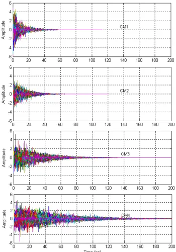
(NLOS). CM1 is based on the LOS transmission and corresponds to the very

short communication range of 0 to 4 m. CM2 is defined for the same range as

in CM1 but with the NLOS transmission. CM3 and CM4 are defined for the

NLOS transmission. However, the communication distances are extended to

4-10 m for CM3 and over 10 m for CM4, respectively.

The IEEE UWB channel model in [26], a slightly modified version of

the S-V model, has been confirmed as a precise channel modelling in reality.

It identifies the number of paths, that is, it determines the number of

multi-path arrivals which reach within 10 dB range from the most powerful arrival.

Moreover, the phase shifts_{θl,k}are restricted to take the values of 0 orπwith

equal probability due to the signal inversion from reflection, and the random

variables _{X_} are also introduced to account for the log-normal shadowing.

(33)

by [26]

h0(t) =X L

X

l=0

K

X

k=0

ak,lδ(t−Tl−τk,l) (2.2)

where L represents the total number of cluster and K represents the total

number of rays within each cluster. It is clear that the arrival time of thelth

clusterTl is the arrival time of the first ray in thelth cluster, for whichτ0,l = 0.

Letψl =Tl−Tl−1 when l≥1 and ψl =Tl when l= 0, respectively. Then the

probability density function (PDF) of the cluster arrival time is given by [26]

as

pψl(t) = Λe−

Λt_, _{l >}₀_. _(2.3)

Similarly, let ϕk,l = τk,l −τk−1,l when k ≥ 1 and ϕk,l = τk,l when k = 0,

respectively. Then the PDF of the ray arrival time in the lth cluster can be

written as

pϕk,l(t) = λe−

λt_, _{k >}₀_. _(2.4)

As known from Section 2.2.1 for the S-V model, ψl and ϕk,l are both

ran-dom independent variables in the Poisson process with Λ and λ being the

arrival rates for clusters and rays within their clusters, respectively. Since

Tl =Pl_x₌₀ψx and τk,l =Pk_y₌₀ϕy,l, the PDFs of Tl and τk,l can be separately

derived as

pTl(t) = Λ·

e−Λt_·_(Λ_t₎l

l! , t >0, l ≥0 (2.5)

and

pτk,l(t) =λ·

e−λt_·₍_λt₎k−1

(k₋1)! , t >0, k≥1. (2.6)

However, for the CM1 channel model, the PDF of Tl at l = 0 equals zero

(34)

suitable to CM2 - CM4 channel models. In addition, the selection ofkexcludes

the value of 0 asτ0,l = 0.

In [26], the coefficients of multipath gain _{ak,l} in (2.2) can be further

represented as ak,l =pk,l·χl·βk,l, where {pk,l}=±1 with equal probabilities

determining the sign of the multipath gain, χl represents the channel fading

associated with thelth cluster andβk,lrepresents the channel fading associated

with the kth ray in the lth cluster. The PDFs of χl and βk,l are separately

given by [28]

pχi(z) =

20

zln 10p2πσ2

1 e−

(20 log10z)2

2σ₁2 _{, z >}_0; _(2.7)

pβk,l(z) =

20

zln 10p2πσ2

2 e−

(20 log10z−µk,l)2

2σ2₂ _{, z >} ₀ _(2.8)

where µk,l = 10 ln Ω_{ln 10}0 − _{Γ ln 10}10Tl − _γ10_{ln 10}τk,l − (σ

2

1+σ22) ln 10

20 , Ω0 is the average energy

of the first path within the first cluster, Γ is the cluster decay rate and γ is

the ray decay rate in the cluster, σ2

1 is the variance of the log-normal fading

term 20 log₁₀χl associated with clusters, and σ22 is the variance of the term

20 log₁₀βk,l associated with rays.

Figure 2.1 shows the channel impulse response for different scenarios.

All the simulation results are obtained based on 600 channel realizations. One

may see that CM1 and CM2 have the similar average delay profiles. However,

the strongest multipath components in CM2 are delayed by about 5 ns in

comparison with those in CM1, due to the NLOS property in CM2. One

can also see from CM3 and CM4 that, increasing the distance between the

transmitter and the receiver results in a longer time spread, compared with

(35)

[image:35.595.143.493.140.641.2]

(36)

2.3 UWB Pulses

The widely used pulsesp(t) for UWB systems include Gaussian pulse, Gaussian

monocycle (the first derivation of a Gaussian pulse) and Gaussian doublet (the

second derivation of a Gaussian pulse), due to their very short pulse durations

and simple functions [20], [29], [30], [31]. All these waveforms have very short

duration of Tp. With Tp on the order of nanosecond, the pulse can resolve

a large number of multipath components and hence, enable rich multipath

diversity provided by these multipath components [21].

The mathematical definition for a typical Gaussian pulse is very similar

to the Gaussian function as

p0(t) =exp

"

−2π

_t

− tn

2 tn

2#

(2.9)

wheretn is the time-scaling factor. Its nth derivation pulse has the form [32]

pn(t) = εn dn dtnexp

"

−2π

_t

− tn

2 tn

2#

. (2.10)

The Gaussian doublet can be modeled by the second derivation of a Gaussian

pulse as

p2(t) =

"

1₋16π

_t

− tn

2 tn

2#

·exp ₋8π

_t

−tn

2 tn

2!

(2.11)

where the pulse is right-shifted by tn

2 ns in the time domain in order to make

the pulse starting time at the system starting point of t = 0 and, therefore,

to make the pulse suitable for the UWB channel model which start from the

“0” point. The pulse energy is Eg =

R_∞

−∞p

2

(37)

0 0.5 1 1.5 2 2.5 3 3.5 4 −0.5

0 0.5 1

Time (ns)

Amplitude

Figure 2.2: The Gaussian doublet in the time domain defined in (2.9).

representation of the Gaussian doublet p2(t) in the frequency domain can be

derived by using a Fourier transform of (2.11) as

Fp2 = F {p2(t)}

=

Z ∞

−∞

"

1₋16π

t₋tn/2 tn

2#

·exp ₋8π

t₋tn/2 tn

2!

·exp(₋j2πf t)dt

= √

πt3

nf2

16 ·exp(jπtnf−

πt2

nf2

8 ). (2.12)

The upper frequencyfH and the lower frequency fL for the Gaussian doublet

can be calculated from eq.(2.12). So thatfH ≈2.3 GHz,fL ≈0.99 GHz and

hence,B =fH −fL ≈1.3 GHz and fc = (fH +fL)/2≈1.7 GHz.

Figure 2.2 and Figure 2.3 exhibit the Gaussian doubletp(t) in the time

domain and in the frequency domain, respectively. In the simulation,tn= 1ns

and thereforeEg = 0.1875. The pulse duration Tp = 1 nsshown in Figure 2.2

also determines the bandwidthB asB _≈ 1

Tp ≈1 GHz, as can be demonstrated

(38)

0 1 2 3 4 5 6 7 8 9 10 0

0.02 0.04 0.06 0.08 0.1 0.12

Frequency (GHz)

Magnitude

Figure 2.3: The Gaussian doublet in the frequency domain defined in (2.12).

However, the power spectral density (PSD) of the most widely used

Gaussian doublet cannot meet the power spectral constraint of the FCC UWB

mask unless a frequency translation is used. Only the PSD of the Gaussian

pulses with an order higher than three can meet this restrictions [33]. Thus, the

pulse shape design for the real UWB system needs to satisfy two conditions:

i) the pulse duration Tp needs to be very short for multiple access and ii) the

energy or power density needs to very low to meet the FCC frequency masks.

References [34] and [35] proposed several novel methods for the UWB pulse

design that meet both requirements discussed as above.

2.4 UWB Communications

As discussed previously in Section 2.3, a single UWB pulse does not contain

any data information by itself. The digital data information need to be added

to this analogue pulse, by means of modulation [13]. In spite of the benefits of

(39)

trans-mission pulse make it very difficult for the traditional modulation schemes for

narrowband systems to be applied for UWB communication systems. Data

rates, spectral characteristics of the transmitted signal, implementation

com-plexity and performance are all significantly related to the employed

modula-tion techniques. Therefore, various UWB modulamodula-tions have been investigated

in the literature to implement suitable modulation schemes for different

sce-narios [36], [37], [38], [39].

Nowadays, the most common modulation technique is pulse position

modulation (PPM) where the data information is modulated by transmitting

at different time instants. Specifically, the pulse is sent before or after a time

scale depending on the value of the digital data. Another common technique

is pulse amplitude modulation (PAM) where the data is modulated by varying

the amplitude of the analogue pulse according to the data value. Other

well-known modulation techniques include, for example, on-off keying (OOK) where

the presence or absence of the analogue pulse determines the data information.

Here, the two most commonly used modulation schemes, PPM and PAM, will

be examined.

2.4.1 Binary PPM

By defining a pulse with arbitrary shape ofp(t), the generic transmitted signal

with the binary PPM (BPPM) in a single-path and single-user environment

can be written as

s(t) = ∞

X

j=−∞

(40)

[image:40.595.201.433.107.376.2]

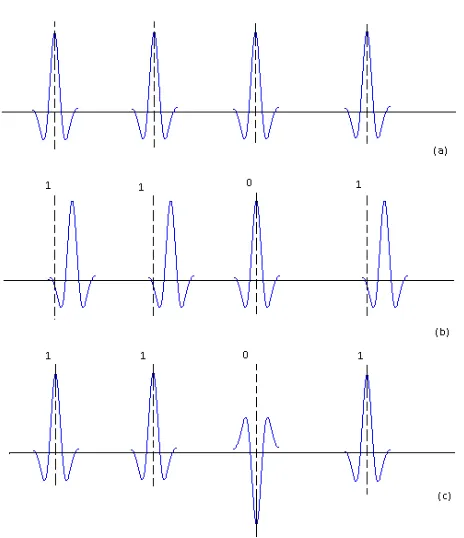
Figure 2.4: Comparison of several different modulation techniques for UWB communications: (a) unmodulated pulses, (b) BPPM and (c) PAM.

where Tf is the frame duration, j is the index of the frame number and Nf

is the number of frames in one symbol. _⌊·⌋ returns the integer part of (_·).

δd_⌊j/Ns⌋ identifies the pulse position with

d_⌊·⌋ being the data information

and δ being the time scale associated with BPPM. The structure diagram of

BPPM is illustrated in Figure 2.4(b), while Figure 2.4(a) shows the

unmod-ulated pulse train for comparison. One can see from Figure 2.4 (b) that the

transmitted pulse containing a digital data bit of ‘1’ is right-shifted byδ; and

the transmitted pulse containing a ‘0’ bit remains.

One can also apply this idea to a M-ary PPM system with various time

shifts. That is, the time shift factor δd_⌊j/Ns⌋ in (2.13) is replaced by τm,j for

(41)

associated with the jth frame [40], [41]. Take a 4-ary PPM system as an

example. One can make τ1 = −0.75Tf, τ2 = −0.25Tf, τ3 = 0.25Tf, and

τ4 = 0.75Tf for one frame. Thus, the four pulses corresponding to the four

mapping situations can be expressed as

s1(t) = ∞

X

j=−∞

p(t₋jTf + 0.75Tf)); s2(t) =

∞

X

j=−∞

p(t₋jTf + 0.25Tf));

s3(t) = ∞

X

j=−∞

p(t₋jTf −0.25Tf)); s4(t) =

∞

X

j=−∞

p(t₋jTf −0.75Tf)).

In this case, each frame can be seen as divided intoM individual sub-slots and

each sub-slot corresponds to a bit sequence. For a single-user UWB system, the

M-ary PPM modulation technique can continuously improve the system

ca-pacity with the increases ofM due to the increased number of bits transmitted

per symbol. However, the capacity differences among the M-ary modulation

schemes with arbitrary M are reduced when the number of system users is

increased. This is due to increased multi-user interference [40].

The PPM modulation scheme benefits from its structure simplicity and

potential high capacity, but it requires extremely fine time control to modulate

and demodulate pulses with an accuracy of a nanosecond.

2.4.2 Binary PAM

With the binary PAM (BPAM), the data is modulated by either inverting the

(42)

with BPAM in a single-path and single-user environment can be written as

s(t) = ∞

X

j=−∞

ϑ_⌊_j/N

f⌋p(t−jTf) (2.14)

where nϑ_⌊_j/N_f_⌋o is the binary codes associated with the data information.

ϑ_⌊_j/N_f_⌋= +1 if the _⌊j/Nf⌋th digital data ‘1’ is transmitted and ϑ_⌊_j/N_f_⌋=−1

if the _⌊j/Nf⌋th digital data ‘0’ is sent. An basic example of BPAM is shown

in Figure 2.4(c). The inverse pulse represents the digital ‘0’ bit, while the

un-inversed pulse represents the digital ‘1’ bit.

Compared with BPPM, the major advantage of using BPAM is due

to the 3 dB gain in the power efficiency [13], [39], [40]. This is due to the

fact that, BPAM can transmit twice the number of pulses and then twice

the data rate over PPM because BPAM does not need to wait for the pulse

transmission. Further discussions about the comparison of BPPM and BPAM

can refer to [42] and [43] for interested readers.

As discussed previously, the modulation schemes can be basically

di-vided into two categories: modelling either the pulse position or the pulse

shape. These schemes all have good performances in a single-user environment,

while in a multi-user system they suffer more interference from other users

ex-isting in the same system. In order to make them suitable for multiple-access

communication systems, spread spectrum techniques are applied and

com-bined with the UWB system in [29]. The most popular spreading spectrum

techniques for UWB systems in the literature are: time-hopping spreading

(43)

Figure 2.5: A typical structure of the UWB TH-SS system with two users.

2.4.3 TH-SS UWB systems

With TH-SS, each pulse is positioned within one frame duration Tf.

Specif-ically, the pulse associated with one user hops in the time domain according

to the pseudorandom TH sequence [29], [44]. Combining the modulation

tech-nique BPPM in eq.(2.13) with the TH-SS scheme, a typical UWB transmitted

signal with TH-BPPM for theuth user is given by

s(u, t) = ∞

X

j=−∞

p(t₋jTf −Tc·cj(u)−δd_⌊_j/N_f_⌋) (2.15)

wherecj(u) is the TH code for thejth frame associated with theuth user,Nf

is the number of frames per symbol and Tc is the chip interval. Herein, each

frame is divided into Nc = T_Tf_c individual chips and the uth user’s TH code

cj(u) is an arbitrary integer in the range of [0, Nc−1] within one frame. Thus,

another time shift of cj(u)·Tc is added to the transmitted signal, compared

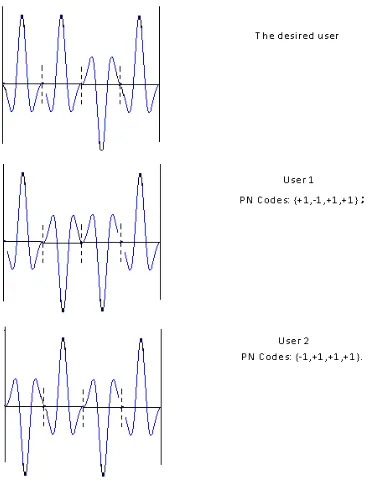
with that employing BPPM only as in eq.(2.13). Figure 2.5 shows a very

(44)

represent the desired users with a TH sequence of [2,4,3] and the dashed lines

represent the interfering users with another TH sequence of [1,2,4]. One sees

that, by utilizing the TH codes, increased number of users can be introduced

in the system with acceptable multiple-access interference (MAI).

Similarly, TH-SS can also be combined with the BPAM scheme. In the

TH-BPAM system, a typical transmitted signal for theuth user can be written

as

s(u, t) = ∞

X

j=−∞

ϑ_⌊_j/N_f_⌋(u)p(t₋jTf −Tc·cj(u)). (2.16)

The difference between the spreading spectrum techniques applied to

the UWB system and the traditional SS techniques defined in [45] is that, the

signal with the former SS schemes does not occupy the entire spectrum. In

the TH-SS UWB systems, each pulse is sent during an arbitrary chip interval

according to the specified TH code. On the other hand, Foerster applied the

DS-SS technique to UWB where one pulse containing the data information is

repeatedly transmittedNctimes in one symbol duration. The DS-SS technique

can reduce the impact of MAI as well [46].

2.4.4 DS-SS UWB systems

Assume that each user has a specific pseudo-noise (PN) sequence with the

length ofNc and hence, the frame durationTf =Nc·Tc where Tc denotes the

spreading gain. A typical transmitted signal for the uth user with DS-BPAM

can be expressed as

s(u, t) = ∞

X

j=−∞

Nc−1

X

n=0

ϑ_⌊_j/N

(45)

[image:45.595.211.397.117.358.2]

Figure 2.6: A typical structure of the UWB DS- system with three users.

where_{cn(u) = ±1} are the spreading codes associated with uth user. In the

DS-SS UWB systems, the frame duration Tf is decreased to a chip duration

Tc and pulses are transmitted successively with a period of Tc. Figure 2.6

illustrates an example of a UWB DS-BPAM system. The PN codes _{cn(u)}

are used herein to change the polarities of the pulses to distinguished different

users.

The system performance is highly related to the PN patterns. With

an appropriate code design, better correlation properties can be achieved in

a multi-user environment [46], [47]. The previous research have demonstrated

that Gold, Kasami, Barker and PN spreading codes are all suitable for UWB

DS-SS systems. Similar investigations for the TH code design in UWB TH-SS

systems are presented in [48].

(46)

been discussed in [49]. The DS-SS scheme is more suitable than the TH-SS

scheme in a multi-user environment, as a higher amount of collision occurs in

the TH-SS scheme.

Eq.(2.15) - eq.(2.17) exhibit the transmitted signal employing various

spread spectrum and modulation techniques, as TH-BPPM, TH-BPAM and

DS-BPAM, respectively. These expressions can be also considered as the

sim-plest format of the UWB transmitted signal which will pass through the

mul-tipath propagation channel to reach the receiver afterwards.

2.5 UWB Receivers

At the receiver, the distorted signal caused by interference and noise needs to

be recovered for the data decision, using the TH-BPAM UWB system as an

example. By substituting eq.(2.2) into eq.(2.16), the received signal for the

uth user can be obtained by

r(u, t) = s(u, t)_∗h0(t)

= ∞

X

j=−∞

L

X

l=0

K

X

k=0

αk,lϑ_⌊_j/N_f_⌋(u)prx(t−Tl−τk,l−jTf −Tc·cj(u))

+ n(u, t) (2.18)

whereprxis the aggregate pulse taking the effects of multipath, multiple-access

and spectrum spreading into account and ‘_∗’ denotes the convolution. n(u, t)

represents the noise for the uth user and it is normally regarded as additive

white Gaussian noise (AWGN).

The receiver design is a major challenge for a UWB system. Several

(47)

re-ceivers such as the RAKE receiver [50] [51], and non-coherent rere-ceivers such as

the transmitted-reference (TR) receiver [52] [53] [54] and the energy detection

receiver [55] [56].

The Rake receiver is often applied in UWB systems to take full

ad-vantage of multipath diversity. However, it is computationally prohibitive to

collect the energies of all the multipath components, as one has to employ an

explicit channel estimator for each multipath component. Therefore,

practi-cal Rake receivers often adopt a limited number of ‘fingers’, at the cost of a

degraded system performance [50], [57].

Instead of using a complicated RAKE receiver, reference [52] proposed

the transmitted reference (TR) receiver, to relax the requirements on

synchro-nization and channel estimation. The traditional TR receiver correlates the

received signal corresponding to the data symbol with the template signal

cor-responding to the reference symbol which is transmitted before the data

sym-bol and hence, this noisy template signal degrades the receiver performance

significantly. Several template designs for reliable data detection in the UWB

TR systems have been developed in [58]. Some template signals in [58] have

a high time-consuming requirement due to their complex template formats.

The energy detector (ED) can provide a simple receiver structure avoiding

recursive algorithms, resulting in significant performance degradation. The

received signal at ED is squared and then thresholded to recover the

transmit-ted data signal. Therefore, the selection of the optimal threshold plays a very

important role in the receiver performance [59], [60].

Interested readers can refer to [61] for further detailed comparison

be-tween coherent and non-coherent receivers in UWB communications. Thus,

(48)

2.5.1 UWB TR Receivers

The attraction of the UWB TR system has been dramatically drawn from both

academic and industrial environments recently. This is due to the improved

system performance with an acceptable of complexity [62]. In the traditional

TR system, the reference (pilot) pulse is transmitted Td seconds before the

data pulse. The part of the received signal corresponding to the reference

information is used to construct the channel template, which is correlated

with the part of the received signal corresponding to the data information for

data detection.

Considering a multi-user UWB TH-BPM system, the transmitted signal

for the ith bit (i.e., the ith symbol) in the uth user is given by

s(u, t) = pεi(u)

Nf−1

X

j=0

[p(t₋jTf −Tc·cj(u))

+ ϑi(u)p(t−jTf −Tc ·cj(u)−Td(u))] (2.19)

whereεi(u) is the signal energy for theith bit in the uth user andTd(u) is the

time interval between data and reference pulses in theuth user. The expression

of the received signal is similar to eq.(2.18) as

r(u, t) = pεi(u)

Nf−1

X

j=0

[h(t₋jTf −Tc ·cj(u))

+ ϑi(u)h(t−jTf −Tc·cj(u)−Td(u))] +n(t) (2.20)

whereh(t) = p(t)_∗h0(t) is the channel response to the transmitted signal. At

(49)

the decision statistic for the ith bit in theuth user can be expressed as [63]

Di(u) =

Nf−1

X

j=0

Ds(j, u) (2.21)

where

Ds(j, u) =

Z jTf+Tc·cj(u)+Td(u)+Tcorr

jTf+Tc·cj(u)+Td(u)

r(u, t)r(u, t₋Td(u))dt (2.22)

with Tcorr being the length of integration interval and r(u, t−Td) being the

channel template. Finally, the data decision is made according to

ˆ

di =

(

0, if Di <0

1, if Di ≥0

(2.23)

where ˆ(_·) denotes the data decision.

Unlike coherent receivers, TR receivers do not require excellent time

synchronization. However, the TR receiver is very sensitive to the integration

position and duration, as all the multipath components are gathered at the

reception stage [64].

2.6 Conclusions

In this chapter, an overview of the basic UWB communication system was

presented, starting with the multipath channel models for UWB. Nowadays,

the most accurate UWB channel model, proposed by the subcommittee of the

IEEE 802.15.3a group for WPANs in 2003, is a slightly different version of

(50)

four categories as CM1 - CM4, according to the transmission type and the

communication distance. The primary parameters that significantly impact

the characteristics of channels were briefly described, including the multipath

fading gain and the multipath arrival times.

A commonly used second-order derivative Gaussian pulse, namely the

Gaussian doublet, was discussed in both the time domain and the frequency

domain. The ultra-short pulse duration in the time domain enables it to

be distinguished from other unwanted multipath components due to its fine

time resolution. On the other hand, this pulse in the frequency domain is

spreaded over an extremely wide bandwidth so that its frequency components

are low enough for the FCC regulations. Therefore, this signal can propagate

very well in the UWB IEEE channels to avoid interference with other existing

communication systems.

Then, two appropriate modulation schemes for the UWB systems, known

as PPM and BPAM, were discussed. Multiple-access techniques for UWB were

also presented. In particular, typical expressions of TH-BPPM, TH-BPAM

and DS-BPAM schemes were provided. The DS-BPAM scheme benefits the

TH-BPAM scheme in a multi-user environment because more collisions

oc-curred in the TH-SS system than in the DS-SS system. Also, the TH-BPAM

scheme always outperforms the TH-BPPM scheme due to the 3 dB gain in

power efficiency. Moreover, a M-ary PPM technology can significantly

im-prove the capacity with a certain number of users.

Finally, a brief description of the UWB receivers was presented.

Nor-mally, the UWB receivers in the literature can be classified as coherent and

non-coherent receivers. Meanwhile, the non-coherent receivers can be further

(51)

energy detector. In a traditional TR system, the received data signal is

corre-lated with the received reference signal for reliable data decision. A complex

channel estimation process is not required for UWB TR systems. Owing to its

structural simplicity and tolerable performance degradation, the TR receiver

has become very attractive recently. In the next chapter onwards, the

opti-mization for the TR receiver to improve its performance in various scenarios

(52)

Chapter 3 Optimization of the Traditional

UWB TR Receiver

3.1 Introduction

As has been discussed previously, the UWB TR receiver was proposed to relax

the requirements on synchronization and channel estimation. These

proper-ties enable the TR receiver to benefit from a simple structure and to be less

computation-consuming. As a result, this also leads to simple

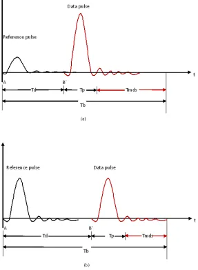
implementa-tions in the TR system. For the traditional TR receiver, the second pulse

corresponding to the modulated signal is transmittedTd seconds after the first

pulse corresponding to the unmodulated signal [53], [62], [65]. The traditional

TR receiver can be also described as an Autocorrelation Receiver (AcR) where

a reference and data pair is sent per frame. The unmodulated signal containing

the reference information is used as a channel template at the correlator, and

the modulated signal contains the data information to detect. A significant

(53)

Stark presented a BER performance analysis of the AcR by using the Gaussian

approximation (GA) in a single-user environment. In [53], Chao and Scholtz

derived the bit error probability (BEP) of the AcR based on knowledge of

the channel properties. In [66], Chao further derived the BEP of the AcR by

using the orthogonal expansion concept instead of the central limit theorem

in the GA for the more accurate theoretical results. In [67], Jia and Kim

de-rived a closed-form expression for the channel-averaged

signal-to-interference-plus-noise ratio (SINR) of the AcR, where multi-user interference (MAI) was

considered. In [68] and [69], Witrisal and Pausini provided the statistical

anal-ysis of the correlation function considering the effect of inter-pulse interference

(IPI), while [68] was based on the Volterra equivalent system model. However,

none of these work has considered the best choice ofTd within the pulse pairs.

This chapter focuses on the optimization of Td in the AcR. Since the

AcR correlates the data signal with the reference signal to capture all the

achievable energies from the multipath, the performance of the AcR suffers

from power loss of the reference signal as well as noise in the template.

Fur-thermore, the value of Td determines the amount of IPI as well as the energy

allocation between the reference signal and the data signal. IfTd is too large,

IPI can be largely eliminated due to the sufficient interval between the

refer-ence and the data signals, but the energy allocated to the data signal could

be too small, assuming fixed total signal energy, such that the useful data

energy captured at the traditional TR receiver may be too small for reliable

detection. This degrades the receiver performance. On the other hand, ifTd is

too small, the inherent IPI could be very significant, although the energy

allo-cated to the data signal is sufficient for reliable detection. This degrades the

(54)

the best tradeoff between interference and energy allocation. Herein, the AcR

is optimized with respect to Td for two criteria, maximization of the channel

achievable capacity and minimization of the system BER. The channel

capac-ity and BER are derived by using an accurate approximation to the SINR.

Numerical results show that the optimized TR receiver can provide significant

gains over the traditional TR receiver in terms of channel capacity and BER.

This chapter is organized as follows. Section 3.2 illustrates the system

model for the traditional TR receiver (AcR). The optimization with respect to

Td using the two criteria (channel capacity and BER) is addressed in Section

3.3. Conclusions are drawn in Section 3.4.

3.2 System Model for the Traditional UWB

TR Receiver

A single-user UWB system is first considered. Therefore, time-hopping or

direct-sequence for multiple access are not used. With BPAM applied, theith

transmitted bit can be expressed as

si(t) =

Nf−1

X

j=0

√

εi

h_√

αgtr(t−jTf) +ϑi

p

(1₋α)gtr(t−jTf −Td)

i

(3.1)

whereNf is the number of frames,j = 0,1,· · · , Nf −1 is the frame index, Tf

is the frame interval, gtr(t) denotes the monocycle pulse with time duration

Tp and energy Eg =

R_∞

−∞g

2

tr(t)dt, εi is the total energy for the ith bit, {ϑi} ∈

{+1,₋1_} with equal probabilities denotes the ith bit associated with the i

data symbol, and Td is the delay between the reference pulse and the data

(55)

function of gtr(t) isRg(∆) = _E1_g

R_∞

−∞gtr(t)gtr(t+ ∆)dt. The energy allocation

factor α is defined as

α= εri

εi

(3.2)

whereεri is the reference energy andTb is the bit duration. Here, it is assumed

that the energy is linearly proportional to the time interval. This assumption is

based on the fact that in general energy equals the product of power and time

and the observation that the average transmission power in wireless device is

often fixed. Although the specific relationship between the energy and the time

may be quadratic or even more complicated, the linear relationship is used as

an example to give general guidance on how to choose the time delay. Using

the same method presented here, one can easily replace this linear relationship

with other specific relationships to find the best time delay for the specific

applications. The investigations will be very similar, as the optimum time

delay can be found from the optimum energy allocation factor by solving an

equation using their relationships. For the reference, since the reference pulse

in one frame continues untilTd seconds later when the data pulse starts, the

total reference time interval can be described as Td·Nf for one bit. Thus,

α = εri

εi

= c·Td·Nf

c_·Tb

= Td·Nf

Tb

(3.3)

where the assumed linear relationship between energy ε and time interval T

as ε = c_·T is used, c is a constant. The bit energy is fixed at εi. Then,

from eq.(3.3), the reference energy per bit is εri = αεi = _Tεi_b ·Td·Nf. Also,

from eq.(3.1), the data energy per bit isεdi = (1−α)εi = _Tεi_b ·(Tb −Td·Nf).

(56)

optimization problem can be described by using Figure 3.1. WhenTdincreases,

from eq.(3.3),αincreases. Since the reference pulse has an amplitude of√αεi,

the reference pulse amplitude increases and therefore, the reference energy

increases. Also, since the data pulse has an amplitude ofp(1₋α)εi, the data

pulse amplitude decreases and therefore, the data energy decreases. On the

other hand, when Td increases, the time space between the reference pulse

and the data pulse increases so that the inter-pulse interference is reduced.

Thus, an optimal Td exists. One notes that the choice of the time delay Td

is equivalent to the choice of α, when Tb is fixed. This selection approach

can be seen as a joint study of reducing the inherent IPI and increasing the

energy allocated to the data signal. In the following, the optimal α will be

determined.

In order to restrict the noise, an ideal bandpass filter with one-sided

bandwidth ofBp= _T1_p (Hz) is applied at the front end of the receiver to remove

excessive noise. Thus, the filtered received signal for the ith transmitted bit

can be expressed as

ri(t) =

Ns−1

X

j=0

√_ε

i

h_√

αh(t₋jTf) +ϑi

p

(1₋α)h(t₋jTf −Td)

i

+ni(t) (3.4)

where h(t) = gtr(t)∗h0(t)∗gre(t) is the equivalent channel response (CR)

to the transmitted waveform, h0(t) is the channel response presented in [26],

gre(t) is the pulse shape of the bandpass filter, and ni(t) is additive white

Gaussian noise (AWGN) with mean zero and variance δ2 ₌ _B

pNo with No

being the one-sided noise power density. The multipath channel model used

here is based on [26] and is assumed to be time-invariant over one observation

(57)

[image:57.595.154.441.190.582.2]

Figure 3.1: The system model of the conventional TR receiver with different

Optimization of transmitted reference receivers in the ultra wide bandwidth system

Optimization of

Transmitted-Reference receivers in

the Ultra-wide Bandwidth System

Shuyi Wang

Thesis

Doctor of Philosophy

School of Engineering

Contents

List of Figures

List of Tables

Acknowledgments

Declarations

List of Publications

Abstract

Abbreviations

Chapter 1

Introduction

1.1

Introduction to Ultra-wide Bandwidth

Sys-tems

1.1.1

Historical development of UWB Technologies

1.1.2

FCC Regulations for UWB

1.1.3

Characteristics of UWB

1.1.4

UWB Applications

1.1.5

Challenges for UWB

1.2

Research Objective

1.3

Contributions to Knowledge

1.4

Thesis outline

Chapter 2

UWB systems

2.1

Introduction

2.2

UWB Channel Models

2.2.1

Saleh-Valenzuela Model

2.2.2

IEEE Model

2.3

UWB Pulses

2.4

UWB Communications

2.4.1

Binary PPM

2.4.2

Binary PAM

2.4.3

TH-SS UWB systems

2.4.4

DS-SS UWB systems

2.5

UWB Receivers

2.5.1

UWB TR Receivers

2.6

Conclusions

Chapter 3

Optimization of the Traditional

UWB TR Receiver

3.1

Introduction

3.2

System Model for the Traditional UWB

TR Receiver