Original citation:
Wandelt, Sebastian, Wang, Jiaying, Leser, Ulf, Deng, Dong, Gerdjikov, Stefan, Mishra,
Shashwat, Mitankin, Petar, Patil, Manish, Siragusa, Enrico, Tiskin, Alexander and Wang,
Wei. (2014) State-of-the-art in string similarity search and join. SIGMOD Record, Volume
43 (Number 1). pp. 64-76.
Permanent WRAP url:
http://wrap.warwick.ac.uk/65568
Copyright and reuse:
The Warwick Research Archive Portal (WRAP) makes this work of researchers of the
University of Warwick available open access under the following conditions. Copyright ©
and all moral rights to the version of the paper presented here belong to the individual
author(s) and/or other copyright owners. To the extent reasonable and practicable the
material made available in WRAP has been checked for eligibility before being made
available.
Copies of full items can be used for personal research or study, educational, or
not-for-profit purposes without prior permission or charge. Provided that the authors, title and
full bibliographic details are credited, a hyperlink and/or URL is given for the original
metadata page and the content is not changed in any way.
Publisher statement:
© ACM, 2014. This is the author's version of the work. It is posted here by permission of
ACM for your personal use. Not for redistribution. The definitive version was published in
SIGMOD Record, Volume 43 (Number 1) 2014.
http://doi.acm.org/10.1145/2627692.2627706
A note on versions:
The version presented here may differ from the published version or, version of record, if
you wish to cite this item you are advised to consult the publisher’s version. Please see
the ‘permanent WRAP url’ above for details on accessing the published version and note
that access may require a subscription.
State-of-the-art in String Similarity Search and Join
Sebastian Wandelt
Knowledge Management inBioinformatics, HU Berlin, Berlin, Germany
Dong Deng
Tsinghua University,Beijing, China
Stefan Gerdjikov
FMI Sofia University,Sofia, Bulgaria
Shashwat Mishra
Special Interest Group inData, IIT Kanpur, Kanpur, India
Petar Mitankin
IICT Bulgarian Academy ofSciences, FMI Sofia University, Sofia, Bulgaria
Manish Patil
Louisiana State University,Louisiana, USA
Enrico Siragusa
Algorithmic Bioinformatics, FUBerlin, Berlin, Germany
Alexander Tiskin
Department of ComputerScience, University of Warwick, United Kingdom
Wei Wang
University of New SouthWales,
New South Wales, Australia
Jiaying Wang
Northeastern UniversityShenyang, China
Ulf Leser
Knowledge Management in Bioinformatics, HU Berlin,
Berlin, Germany
ABSTRACT
String similarity search and its variants are fundamental problems with many applications in areas such as data integration, data quality, computational linguistics, or bioinformatics. A plethora of methods have been de-veloped over the last decades. Obtaining an overview of the state-of-the-art in this field is difficult, as results are published in various domains without much cross-talk, papers use different data sets and often study subtle variations of the core problems, and the sheer number of proposed methods exceeds the capacity of a single research group. In this paper, we report on the results of the probably largest benchmark ever performed in this field. To overcome the resource bottleneck, we or-ganized the benchmark as an international competition, a workshop at EDBT/ICDT 2013. Various teams from different fields and from all over the world developed or tuned programs for two crisply defined problems. All algorithms were evaluated by an external group on two machines. Altogether, we compared 14 different
pro-grams on two string matching problems (k-approximate
search and k-approximate join) using data sets of
in-creasing sizes and with different characteristics from two different domains. We compare programs primarily by wall clock time, but also provide results on memory us-age, indexing time, batch query effects and scalability in terms of CPU cores. Results were averaged over sev-eral runs and confirmed on a second, different hardware platform. A particularly interesting observation is that disciplines can and should learn more from each other,
with the three best teams rooting in computational lin-guistics, databases, and bioinformatics, respectively.
Keywords
String search, String join, Scalability, Comparison
1.
INTRODUCTION
Approximate search and join operations over large col-lections of strings are fundamental problems with many
applications. String similarity search is used, for
in-stance, to identify entities in natural language texts [29], to align DNA sequences produced in modern DNA se-quencing with substrings of a reference genome [16, 17], or to perform pattern matching in time series repre-sented as sequences of symbols [10]. String similarity joins are building blocks in the detection of duplicate Web pages [13], in collaborative filtering [2], or in entity reconciliation [7]. Research in this field dates back to the early days of computer science and the area is still highly active today. Literally hundreds of methods have been proposed.
For string similarity search and join, fundamental tech-niques include seed-and-extend methods (turning sim-ilarity search into an exact search problem of smaller strings, e.g. All-Pairs [2], ED-Join [31], and PPJoin [32]), partitioning techniques (e.g. Pass-Join [15], NGPP [29], and PartEnum [1]), prefix-filtering methods (e.g. Trie-Join [8] and PEARL [23]), and other methods (e.g. M-Tree [5], LSH [12], SSI [9], and FASTSS [25]).
NGPP Ed-Join Pass-Join Trie-Join
PartEnum All-Pairs PPJoin
FastSS
M-Tree
LSH
[image:3.612.91.276.70.140.2]SSI Pearl
Figure 1: Recent work on string similarity search and join with edit distance constraints. An edge from method M1 to M2 visualizes that M2 was
found to be superior to M1. Marked approaches
are non-dominated, i.e. not reported strictly slower than any other method.
scientific disciplines, the most important ones proba-bly being algorithms for pattern matching, computa-tional linguistics, bioinformatics, and database / data integration. There are subtle differences between the problems being studied, for instance varying in the con-crete similarity measure (edit distance, Jaccard, Ham-ming etc.), the type of string comparisons (global or local alignment, approximate substring search etc.), the amount of indexing being allowed (online in the queries and/or the database). Methods often are tuned for spe-cific ranges of allowed error thresholds or query lengths, specific hardware properties, specific alphabet sizes, or specific distributions of errors. Though newly published methods mostly compare to some prior works, selection of these works is often suboptimal and comparisons are carried out on different data sets; data sets all too often are not made publicly available, which means that re-sults are not reproducible. In Figure 1, we show existing evaluation results for the most relevant work on string similarity search/join with edit distance constraints. As a consequence of the heterogeneity of approaches and problems, the lack of common benchmarks, and the dis-persal of research in different communities, today it is hardly possible to choose the best algorithm for a given problem.
In this work, we report on the (to the best of our knowl-edge) most comprehensive benchmark in two specific
string similarity match problems to date:k-approximate
search and k-approximate join (with k as an edit
dis-tance threshold; see below for exact definition). We
organized this benchmark using a rather uncommon
ap-proach: TheInternational competition on Scalable String
Similarity Search and Join (S4)1 held as a workshop
in conjunction with EDBT/ICDT 2013. We made an open, world-wide call for contributions and provided crisp task definitions, a loose hardware specification and example data. Nine teams from different communities participated, including databases, natural language pro-cessing, and bioinformatics. Thus, for the first time, we were able to evaluate different highly competitive imple-mentations of search and join algorithms on the same evaluation platform (hardware, operating system, and datasets). In addition, organizing the benchmark as a competition, where teams developed and tuned their
1http://www2.informatik.hu-berlin.de/~wandelt/
searchjoincompetition2013/
own programs independently, allowed us to compare original and optimized programs instead of unverified and potentially unoptimized re-implementations. All submitted programs were tested on different datasets (DNA sequences and geographical names) of different sizes (a few KB up to a few GB) with different error
thresholds (edit distancekbetween 0 and 16). We
per-formed experiments in two different hardware settings: a commodity PC with 8 cores/64 GB RAM and a server with 80 cores/1 TB RAM. For the top performing pro-grams we performed additional analyses with different number of threads to investigate the possibility to par-allelize algorithms. Furthermore, we compared submis-sions with a number of publicly available algorithms of groups that did not participate, showing that the best ranked programs from our competition are several or-ders of magnitude faster. Altogether, 14 different pro-grams or configurations were evaluated with differences in runtime of factors of more than 1000 between the fastest and slowest program. We are confident that our results give a fairly representative picture of the state-of-the-art in string similarity search. The evaluation of all programs and datasets took more than three months of raw processing time.
The wealth of experiments we performed and the sig-nificant number of programs we compared allows us to draw several interesting conclusions about scalability, batch procession effects, index size, main memory us-age, and the possibility to parallelize techniques. The purpose of this paper is not only to report on ef-ficiency of algorithms in string similarity search, but also to promote competitions as an effective, joyful, and comprehensive means to evaluate the state-of-the-art on a given problem. Actually, competitions are quite com-mon in many related disciplines, such as information ex-traction, information retrieval, data analysis etc., but, to our knowledge, represent a novel approach within the database community. The only comparable effort we are aware of is the SIGMOD programming contest. How-ever, it only addresses graduates and the focus is more on education (and probably recruitment). In contrast, the main purpose of S4 was to identify the fastest meth-ods available. Clearly, the most critical point for a com-petition like S4 is the measurement of wall clock time, which is dependent on the concrete implementation and the machine being used for measurements, instead of quality metrics independent of the concrete implemen-tation and evaluation environment (such as precision or recall). We will expand on this issue in Section 6. The remainder of this paper is organized as follows. We describe the concrete problems we benchmarked, the datasets, and the benchmarking methodology in Sec-tion 2. All submitted methods are briefly presented in
Section 3. Evaluation results for approximate string
1. Initial call for contributions (June 2012) 2. Letter of intent (November 15th, 2012) 3. Publication of test data (November 16th, 2012) 4. Tuning phase (November 16th, 2012 - January 20th, 2013) 5. Final submission of executables (January 20th, 2013) 6. Evaluation (January 2013 - March 2013)
7. Workshop (March 22nd, 2013)
[image:4.612.83.290.73.177.2]8. Post-workshop analysis (March 2013 - July 2013)
Figure 2: Phases of the competition
2.
BACKGROUND
We define the problems of approximate string search-ing and approximate strsearch-ing join. Our competition and evaluation methodology is introduced together with a description of datasets and evaluation environments.
2.1
Formal problem statement
Definition 1 (Strings). Astringsis a finite
se-quence of symbols over an alphabet Σ. The length of a
string s is denoted by |s|and the substring starting at
positioniwith lengthnis denoted bys(i, n). We write
s(i) as an abbreviation for s(i,1). All positions in a
sequence are zero-based, i.e., the first character ofs is
s(0).
As a distance function between two strings we use un-weighted edit distance for different error thresholds k.
Definition 2 (String similarity). Given strings
sandt,sisk-approximately similar tot, denoteds∼k
t, if and only ifscan be transformed intotby at mostk
edit operations. The edit operations are: replacing one
symbol in s, deleting one symbol froms, and inserting
one symbol intos.
We investigate two problems: string similarity search and string similarity join.
Definition 3 (Similarity search). Given a
col-lection of stringsS={s1, ..., sn}, a query stringq, and
an edit distance thresholdk, the result of string
similar-ity search ofqin S is defined as
SEARCH(S, q, k) ={i|si∈S∧si∼kq}.
For instance, given a collectionS={ACA, T GA, AC},
a query stringq=ACA, andk= 1, the result of string
similarity search isSEARCH(S, q, k) ={1,3}.
Definition 4 (Similarity (self) join). Given a
collection of stringsS={s1, ..., sn}and an edit distance
thresholdk, the result of string similarity self-join ofSis
defined asJOIN(S, k) ={(i, j)|si∈S∧sj∈S∧si∼k
sj}.
For instance, the result of a string similarity self-join
on data setS from above withk= 1 isJOIN(S,1) =
{(1,1),(1,3), (2,2),(3,1),(3,3)}. Note that we explic-itly include the reflexive and symmetric closure in our definition. We note that a self-join is comparable to a join between two different sets as we make no assump-tions about the a priori average level of similarity of the strings in a set. In the following we will often use the term join instead of self-join.
2.2
Competition and methodology
This competition brought together researchers and prac-titioners from database research, natural language pro-cessing, and bioinformatics. The challenge for all par-ticipants was to perform string similarity search and join over unseen data and query sets with varying
er-ror thresholds k as fast as possible. The call for the
competition was circulated by email through various lists addressing the different areas dealing with string matching, in particular databases, algorithms, compu-tational linguistics, and bioinformatics. We also con-tacted directly a few dozen researchers known for their contributions to the field. The different phases of the competition are shown in Figure 2.
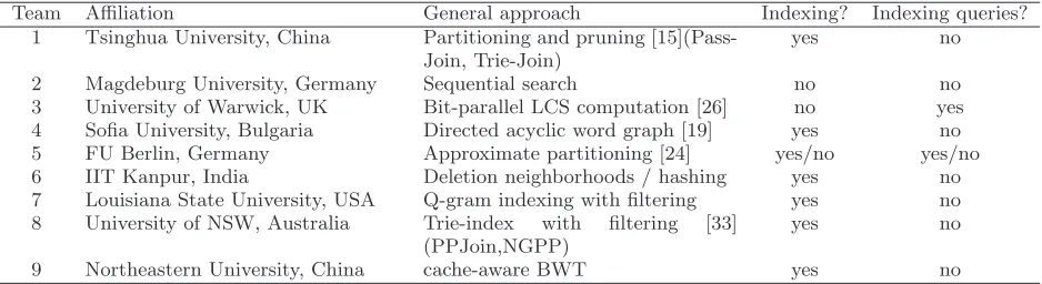
In total we received initial expressions of interest from 22 teams, out of which 11 teams officially submitted
a program. One team failed to hand in a complete
paper describing their approach on time, and another group withdrew shortly before the final deadline. Thus, we eventually compared programs from 9 teams (see Table 1). All these teams gathered at a workshop co-locates with EDBT/ICDT 2014 in Genoa, where each team presented its approach and the results of our eval-uation were discussed. This format led to a workshop in the best sense of the word - as all presentations es-sentially covered the same problems, talks were highly focused and intensive discussions and exchanges of ideas emerged naturally. We also organized culinary prices for the best teams which were immediately shared with the entire audience.
We succeeded in reaching out to different research com-munities: two teams have their home in bioinformat-ics, two in computational linguistbioinformat-ics, one in algorithms/ computational complexity, and the remaining four are best described as database groups. Contributions came from four continents and seven countries. At least six teams (Team 1, 3–5, 7–9) published highly influential papers on string matching problems before [15, 19, 22, 24, 26, 28, 33], while two teams (Team 2 and Team 6) can be considered as newcomers. As Table 1 shows, the techniques used cover a broad range and thus subsume
a large fraction of previous research in k-approximate
string matching. Out of the five non-dominated meth-ods in Figure 1, four methmeth-ods are directly represented by corresponding authors in our competition.
The competition consisted of two tracks:
Track 1: Given a set of stringsS, a query stringqand
an error thresholdk, computeSEARCH(S, q, k).
Track 2: Given a set of stringsSand an error threshold
k, computeJOIN(S, k).
Team Affiliation General approach Indexing? Indexing queries?
1 Tsinghua University, China Partitioning and pruning
[15](Pass-Join, Trie-Join)
yes no
2 Magdeburg University, Germany Sequential search no no
3 University of Warwick, UK Bit-parallel LCS computation [26] no yes
4 Sofia University, Bulgaria Directed acyclic word graph [19] yes no
5 FU Berlin, Germany Approximate partitioning [24] yes/no yes/no
6 IIT Kanpur, India Deletion neighborhoods / hashing yes no
7 Louisiana State University, USA Q-gram indexing with filtering yes no
8 University of NSW, Australia Trie-index with filtering [33]
(PPJoin,NGPP)
yes no
[image:5.612.72.541.71.199.2]9 Northeastern University, China cache-aware BWT yes no
Table 1: Teams which participated in the competition
15,000 100
150,000 1,000
1,500,000 10,000
5,000,000 20,000
15,000,000 100,000
[image:5.612.78.537.234.333.2]20,000,000 200,000
|dataset| |queries|
10,000 1,000
50,000 5,000
100,000 10,000
Geonames
15,000
150,000
1,500,000
5,000,000 15,000,000
100
1,000
10,000 20,000
100,000
10 100 1,000 10,000 100,000 1,000,000 10,000,000 100,000,000
TINY SMALL MEDIUM LARGE HUGE READS
|dataset| |queries|
10,000
50,000
100,000
500,000
1,000,000
1,000
5,000 10,000
50,000
100,000
100 1,000 10,000 100,000 1,000,000
TINY SMALL MEDIUM LARGE HUGE CITIES
|dataset| |queries|
Figure 3: Size of dataset and number of queries used for evaluation (READS and CITIES)
and a maximum of 48 GB of main memory. Details on CPU, clock rate, cache sizes, disks etc. were not pro-vided to prevent hardware specific tuning; note that this implies that further improvements could be possible tak-ing the specific hardware into account [20]. Programs were allowed to have two phases, one for indexing the data set, and one for evaluating a set of queries on the set (or the index). The main evaluation criterion was measured wall clock time. In general, we ranked pro-grams based on average runtime over three independent runs; variations in runtime were very low and are not re-ported here. If programs ran much longer than most of the competitors, experiments were only performed once. We also measured the indexing time and report it here, but we did not take it into account for ranking.
2.3
Datasets
We used two different types of datasets, for evaluation in both tracks, to cover different alphabets and string
lengths. Each type of dataset contains five distinct,
highly-similar datasets of increasing size, for evaluating scalability.
READS: These data sets contain reads obtained from a human genome. The data is characterized by a small alphabet (5 symbols) and quite uniform length of strings (around 100 symbols per string).
CITIES: These data sets are based on geographical
names taken from World Gazetteer. The data
is characterized by a larger alphabet (around 200 symbols) and non-uniform length of strings (5-64).
Considered values for k depend on the dataset. For
READS, we announced and used k ∈ {0,4,8,12,16};
for CITIESk∈ {0,1,2,3,4}. Thus the maximum error
rate for READS is around 16 and for CITIES around
4
5. The size of each dataset and the number of queries
for Track 1 are shown in Figure 3. For READS, the number of reads starts with 15,000 (TINY) and ends with 15,000,000 (HUGE). For CITIES, the number of cities starts with 10,000 (TINY) and ends with 1,000,000 (HUGE). For READS and CITIES, the maximum num-ber of queries in HUGE is 100,000.
2.4
Evaluation Environments
After the development phase of the competition, partic-ipants submitted their final programs which were eval-uated on two different platforms.
System 1: A computer with 8 cores (processor: AMD FX-8320) and 64 GB RAM. The operating system (Fedora Scientific 17 x86 64) was installed on a SSD with 128 GB. The SSD contained the datasets as well as the programs. Each program serialized its results to an external USB 3.0 hard disk with 3 TB. This system was announced beforehand and results for this system were used for ranking.
System 2: A server with 80 cores (processors: Intel Xeon CPU E7 - 4870) and 1 TB RAM. The op-erating system was openSUSE 12.1 x86 64. All datasets, programs, and serialized results were put on a local hard disk with a total storage capac-ity of 10 TB. This system was introduced only during evaluation for (a) performing experiments with more cores / memories and for (b) confirm-ing results on a separate hardware with different architecture and CPUs.
inves-tigating the scalability with the number of threads (for top performing methods on System 1). In our evalua-tion below, we will menevalua-tion explicitly if System 2 was used.
3.
METHODS
This section describes the methods used by each team in their submissions to the competition.
3.1
Team 1
PassJoin (Tsinghua University) adopts a partition-based framework for string similarity search and joins. The
ba-sic idea is that given two datasetsRandS, and an edit
distance thresholdk, each string inRis split intok+ 1
disjoint segments. For each string inS, PassJoin checks
if it contains any substring matching the segments ofR.
If no, PassJoin prunes the string; otherwise the string and those strings whose segments match the substrings of the string are verified. There are two challenges in
the partition-based method. The first one is how to
select the substrings. A position-aware substring tion method and a multi-match-aware substring selec-tion method have been proposed. It has been proven the multi-match-aware substring selection method selects the minimum number of substrings. And it is the only way to select the minimum number of substrings when
the string length is longer than 2∗k+ 1. The second
one is how to verify each candidate pair. PassJoin uses a length-based verification method, an improved early termination technique, and an extension-based verifica-tion method.
Team 1 submitted two programs: Program 1 Aand
Program 1 B. Both programs of Team 1 were evalu-ated for both tracks and both datasets.
3.2
Team 2
Team 2 (Magdeburg University) tries to outperform con-ventional index-searches by a sequential search
algo-rithm. Starting from a naive algorithm for
comput-ing edit distances, several optimizations are introduced. Calculation of the edit distance is improved by using length-heuristics. If the computation of a dot matrix cannot be avoided, the program applies several heuris-tics to prune the search space early. Further optimiza-tions include the use of reference-based semantics over value-based semantics and the use of simple data types. They devise simple scheduling strategies depending on the current workload.
Team 2 submitted only one program: Program 2 A,
which was evaluated for Track 1 only.
3.3
Team 3
The Waterfall algorithm of Team 3 (University of War-wick) solves the competition challenge without index-ing or any other preprocessindex-ing of the database strindex-ings. First, a reduction of the edit distance problem to the longest common subsequence (LCS) problem between the database string and the query string, both
suit-ably modified, is applied. The strings’ LCS score is
then computed by a bit-parallel algorithm, based on [6]. This technique is extended so that a database string can
be tested simultaneously against multiple query strings, by a subword-parallel technique similar to that of [14], which was further developed in the waterfall algorithm. Due to the self-imposed restriction of not preprocess-ing the database, the algorithm runs significantly slower than other competitors, which do index the database strings before answering the queries. However, the ap-proach chosen by Team 3 can prove useful in a situation where input preprocessing is not possible. Such a sit-uation occurs e.g. when the string database is replaced by a continuous stream of input strings, each of which needs to be matched against a small set of query strings in real time.
Team 3 submitted only one program: Program 3 A,
which was evaluated for both tracks and both datasets.
3.4
Team 4
The WallBreaker of Team 4 (Sofia University) is a new sequential algorithm for the similarity search problem in a finite set of words. It reduces and essentially over-comes the wall-effect caused by the redundantly gener-ated false candidates. To achieve this the query is split into smaller subqueries with smaller threshold. This al-lows to start with an exact match and then extend these exact matches to longer candidates whereas the thresh-old increases slowly in a stepwise manner. In order to implement this idea in practice two kind of resources are used: (i) a linear space representation of the infixes in the finite set of words that enables a left/right extension of an infix in constant time per character; and (ii) effi-cient filters, universal Levenshtein automata [18], sych-norised Levenshtein automata [19] and standard Ukko-nen filter [27], that prune the unsuccessful candidates as soon as a clear evidence for this occurs. In the in-dex structure information about the possible lengths of longest/shortest left/right possible extensions are en-coded. This information is then used as an additional length-filter.
As a result a breaking-the-wall-effect is achieved. In the beginning the WallBreaker considers only small neigh-borhoods of short words which keeps the searching space modest. Afterwards, while increasing the potential size of the neighborhoods, longer infixes are generated that are much more informative than shorter ones and sup-press the searching space for their own sake. For further details the reader is refered to [11], where besides the standard Levenshtein edit-distance also the generalized Levenshtein edit-distance is handled.
Team 4 submitted two programs:
Program 4 A: It uses16threads, the additional length-filter, and applies universal Levenshtein automata for
thresholds≤5, and synchronised Levenshtein automata
for thresholds≤3.
Program 4 B: It uses 16 threads, ignores the addi-tional length-filter, and applies universal Levenshtein
automata for thresholds≤5, and synchronised
Leven-shtein automata for thresholds≤3.
3.5
Team 5
The methods of Team 5 (FU Berlin) are variations of those applied in Masai [24], a tool for mapping high-throughput DNA sequencing data. First an online so-lution for computing edit distances using a banded ver-sion of the Myers bit-vector algorithm [21] is proposed. Team 5 is able to check in timeO(k+1)(wn+|Σ|), where
w is the CPU word size and Σ the string alphabet, if
two strings of length m and n (w.l.o.g. m < n) are
within edit distance k. Then they propose to index
multiple queries in a radix tree and backtrack them into the radix (or suffix) tree of the database. In practice, radix (and suffix) trees are replaced by simpler radix (and suffix) arrays. Multiple backtracking is parallelized with static load balancing and work queues. Finally, as proposed by Navarro and Baeza-Yates [21], a filter-ing method partitionfilter-ing queries into approximate seeds is implemented. Such a filtering method combines the previous two methods and works well up to moderate error rates. The programs are implemented in C++ and OpenMP using the SeqAn library.
Team 5 submitted four programs:
Program 5 A: An online algorithm.
Program 5 B: Partitioning with minimum seed length (10 for READS, 4 for CITIES)
Program 5 C: Partitioning with minimum seed length (13 for READS, 5 for CITIES)
Program 5 D: Partitioning with minimum seed length (15 for READS, 6 for CITIES)
3.6
Team 6
The submission of Team 6 (IIT Kanpur) uses deletion
neighborhoods [25]. Ak-neighborhood is generated for
every strings∈S. Every string in thek-neighborhood
is referred to as a key. The underlying index structure is a hash-table which maintains an inverted index on
the keys. In order to circumvent the large space
re-quirement, the program only indexes anLs-length
suf-fix for each key. Given a query string q and an edit
distance thresholdk, first thek-neighborhood ofq,Nq,
is generated. The list corresponding to every key in
Nq is obtained from the index structure. A union of
these lists is guaranteed to be a superset of the answer setSEARCH(S, q, k). For each string s in the gener-ated candidate list, the program uses a length-threshold
aware distance computation to verifys. In a multi-core
environment, the program partitions the entire
work-load into k equal parts and each part is handled by a
single, dedicated thread. Team 6’s idea is that dele-tion neighborhoods offer a powerful, selective signature scheme to process edit distance queries. Team 6 only
participated in Track 1 of the competition. Further,
since deletion neighborhoods are only suited for
scenar-ios with larger alphabet size, Team 6’s submission
Pro-gram 6 Awas only evaluated on CITIES dataset.
3.7
Team 7
The index structure of Team 7 (Louisiana State Uni-versity) consists of a generalized suffix tree (GST) and a two-level wavelet tree (WT) on its leaves. The first level WT maintains an array of starting positions of all
suffixes of GST. For each leaf of this WT, another WT for the difference between the starting position of the suffix and the string length to which it belongs to is
maintained. Givenτ,r, Team 7 obtains τ+k disjoint
partitions of r aiming to balance selectivity of count
filtering and frequency of partitioned segments. Then GST and WT are used to obtain inverted list of each partition pre-filtered by “Position Restricted Alignment” that combines the well-know length and position filters. All inverted lists are then merged to retrieve the strings similar tor.
Team 7 submitted only one program: Program 7 A,
which was evaluated for Track 1 with READS only.
3.8
Team 8
Team 8 (University of NSW) presents a solution based on tries, which have the advantages of small indexing space, freeness of verification, and computation sharing among strings with common prefixes. The method pro-posed is a simple adaptation of trie-based error-tolerant prefix matching [30]. Existing trie-based methods pro-cess a query by incrementally traversing the trie and maintaining a set of trie nodes (called active nodes) for each prefix of the query. One common drawback is that they have to maintain a large number of active nodes. Instead, Team 8 records only a small number of po-tentially feasible nodes as ”active nodes” during query processing, which reduces the overhead of maintaining nodes and reporting results. In addition, Team 8 char-acterizes the essence of edit distance computation by a novel data structure named edit vector automaton, which substantially accelerates the state transition of active nodes, and therefore, improves the total query performance. Naive parallelization is added to exploit multi-core CPUs.
Team 8 submitted only one program: Program 8 A,
which was evaluated for Track 1 with CITIES only.
3.9
Team 9
BWTSearcher of Team 9 (Northeastern University) takes advantage of a cache-aware multicore framework using Burrows-Wheeler-Transform [4]. BWTSearcher segments the whole collection of database sequences to fit to the CPU cache lines. The approximate string search algo-rithm is based on a partition approach. The query is
decomposed intoτ + 1 chunks. If P matches the text
with at mostτerrors, at least one of the parts will match
a substring of the text exactly. A new data structure called BWTPA is proposed to find the matching
can-didates. Length filter and position filter are used to
prune the candidates. Team 9 proposed a reversed seg-ment trie to merge the identical segseg-ments, which can save much duplicated computation. In addition, a look ahead algorithm is developed to support bounded edit distance and improve the verification of the candidate strings. BWTSearcher can search on any dataset, but is not optimized on DNA data, yet.
Team 9 has only one participating program: Program
Prog. I S I S I S I S I S 1_A 0.4 0.2 1.1 0.4 10.3 4.3 34.0 24.5 108.0 312.1 1_B 0.4 0.2 1.2 0.4 10.5 9.5 33.6 64.9 100.9 924.7
2_A 0.1 2.4 1.3 185.7 - - -
-3_A 0.0 1.5 0.0 4.5 0.3 289.8 0.7 1,979.8 2.0 30,898.0 4_A 2.5 0.5 29.3 0.2 291.0 4.6 872.5 24.6 2,251.8 232.5 4_B 1.7 0.3 23.0 0.5 235.2 5.4 710.3 27.8 1,754.5 249.0
5_A 0.0 0.5 0.1 23.9 0.9 2,802.1 - - -
-5_B 1.40.1 2.4 0.7 15.8 8.7 55.4 51.6 192.2 580.8 5_C 1.40.1 2.4 1.7 15.7 31.4 55.3 95.8 193.9 761.2 5_D 1.40.1 2.3 2.7 15.5 52.5 55.7 138.9 193.7 900.3 7_A 0.5 0.5 1.1 0.4 168.4 13.2 567.8 62.9 2,710.9 1,587.8 9_A 0.3 0.2 2.4 9.2 26.5 532.5 85.6 3,269.4 465.6 42,866.6
[image:8.612.77.287.71.200.2]TINY SMALL MEDIUM LARGE HUGE
Figure 4: Indexing (I) and search (S) times for
dif-ferent READS datasets (Track 1,kvaries per query)
[time in seconds].
4.
EVALUATING APPROXIMATE STRING
SEARCH METHODS
In the following section we report results for all sub-missions for Track 1: approximate string search. We present results for READS datasets first and then for CITIES.
4.1
Similarity Search for READS
In Figure 4, we show the indexing and search times
for the READS dataset and random values fork (for
each query in the dataset we have assigned a random
number out of{0,4,8,12,16}). For READS-TINY and
READS-SMALL most of the programs compute the re-sults within a few seconds, with two exceptions. 2 A, the index-less approach, needs already 185 seconds for answering READS-SMALL. For READS-MEDIUM, 2 A did not compute a result within several hours, so it was not evaluated on the larger datasets. Program 5 A, an-other index-less approach, needs 23.9 seconds for READS-SMALL and around 45 minutes for READS-MEDIUM. Therefore, 5 A was not tested on READS-LARGE and READS-HUGE.
The fastest programs for READS-HUGE are 4 A and 4 B, taking 232.5 and 249.0 seconds, respectively. The third program is 1 A, which needs 312.1 seconds. How-ever, the indexing time of 1 A is around 20 times shorter than the indexing time for 4 A and 4 B. Programs 1 B, 5 B, 5 C, and 5 D need 10 to 15 minutes for READS-HUGE. Program 3 A, which does not use an index struc-ture, already needs 8 hours to compute all solutions for READS-HUGE.
In Figure 16, we show search times for different values of k and the dataset READS-MEDIUM. The indexing time for all the programs is independent of the value of
k, and is shown in Figure 4. Except 3 A and 9 A, all
programs can compute the results set fork≤8 within
few seconds. The best program fork= 16 is 4 A,
need-ing only 17.8 seconds, followed by 4 B and 1 A. For all values of k, 4 A is among the fastest programs, only
clearly outperformed by 1 A fork= 12.
We have further analyzed the effect of batch-processing
for all programs for READS-MEDIUM andk= 4,
ex-cept 2 A. In Figure 15, the average time per query for different numbers of queries is shown. It can be seen
READS- Prog. I S I S I S
1_A 16.6 4.1 15.8 1.8 14.6 1.2
4_A 510.6 4.9 527.2 2.0 639.4 1.5
5_B 25.0 14.7 24.9 17.4 18.1 16.6
1_A 47.4 26.3 48.3 10.9 47.8 7.0
4_A 1,851.3 27.0 1,518.6 12.8 1,740.8 8.1
5_B 93.7 80.0 66.1 81.8 66.0 91.2
1_A 131.8 371.7 134.9 137.7 131.1 82.1
4_A 4,290.4 245.3 3,718.7 87.2 4,096.2 42.8 5_B 301.2 1,237.5 240.3 1,186.4 2,172.2 1,403.7 LARGE
HUGE
8 threads 24 threads 80 threads
[image:8.612.325.535.73.170.2]MEDIUM
Figure 5: Search times for READS on System 2 [time in seconds].
Prog. I S I S I S I S I S
1_A 0.1 0.5 0.1 0.4 0.2 0.9 0.9 18.2 1.9 59.9
1_B 0.1 0.4 0.1 0.4 0.2 0.9 0.9 17.7 1.7 46.8
2_A 0.0 0.5 0.0 4.0 0.1 23.6 0.2 228.3 -
-3_A 0.0 1.5 0.0 3.0 0.0 6.1 0.1 41.2 0.2 109.6
4_A 2.3 0.2 3.9 0.7 7.0 1.6 25.0 28.5 39.7 69.2
4_B 1.1 0.5 3.9 0.7 7.0 1.6 24.5 28.4 39.9 67.3
5_A 0.0 2.0 0.0 39.0 0.0 176.5 0.1 3,623.9 -
-5_B 2.4 1.1 2.4 14.6 2.5 53.8 2.7 1,018.9 3.1 4,903.0 5_C 2.4 1.1 2.4 13.6 2.4 44.7 2.7 1,088.8 3.2 4,387.4 5_D 2.4 1.6 2.4 14.6 2.5 43.2 2.7 1,062.3 3.1 3,097.0 6_A 13.0 0.5 63.2 1.3 126.3 2.8 562.4 16.0 1,206.3 248.3
8_A 0.0 0.5 0.1 1.4 0.2 5.4 1.0 107.9 2.0 445.5
9_A 0.1 0.5 0.1 0.9 0.2 2.5 1.1 15.2 1.6 137.5
TINY SMALL MEDIUM LARGE HUGE
Figure 6: Indexing (I) and search (S) times for dif-ferent CITIES datasets [time in seconds].
that for most programs, the average query answering time per query is reduced, if the number of queries is increased. For a large number of queries, the programs of Team 1 and Team 4 have the shortest time per query. We have further evaluated the three top-performing pro-grams on our second evaluation environment System 2 with a different number of threads. Each program was preset to use 8, 24, and 80 threads, respectively. In Fig-ure 5, the results of the evaluation are shown. It can be seen that 1 A and 4 A scale quite well with the number of threads: if the number of threads is increased by 3 (8 to 24), the search time is reduced by a factor larger than 2. The improvement from 24 threads to 80 threads is not as big any more. For 5 B there is almost no effect when increasing the number of threads. Their multiple backtracking algorithm is not straightforward to par-allelize and the static load-balancing approach doesn’t scale well. In this scenario it is probably easier to aban-don multiple backtracking and go back to ”standard” single backtracking, to allow a query-by-query paral-lelization.
4.2
Similarity Search for CITIES
In Figure 6, we show the indexing and search times
for the CITIES dataset and random values fork. For
[image:8.612.325.534.213.342.2]CITIES-CITIES- Progr. I S I S I S
1_A 0.21 0.57 0.22 0.24 0.27 0.19
4_A 10.25 0.95 10.26 0.38 10.31 0.23
5_B 0.77 158.15 1.20 133.68 1.36 103.95
1_A 1.123 12.84 1.042 5.341 1.143 3.222
4_A 33.283 17.68 33.353 7.297 33.686 4.377 1_A 2.225 43.615 2.226 19.679 2.247 11.529 4_A 52.903 57.473 53.53 28.283 53.175 21.057 HUGE
LARGE
8 threads 24 threads 80 threads
MEDIUM
Figure 7: Search times for CITIES on System 2 [time in seconds].
HUGE within several hours. Indexing times are quite short for all programs, except 6 A, which almost spends 20 minutes on indexing CITIES-HUGE.
The fastest program for CITIES-HUGE is 1 B,
need-ing 46.8 seconds. It is closely followed by 1 A, 4 A,
and 4 B. The programs of Team 5 are the slowest for CITIES, which probably means that their approach is better suited to deal with small-alphabets.
In Figure 17, the search times for CITIES-MEDIUM and different values of k are shown. Programs 1 A and 1 B are always among the fastest.
We have further evaluated the three top-performing pro-grams on our second evaluation environment System 2 with a different number of threads. In Figure 7, the sults are shown. The results are very similar to the re-sults of READS: Program 1 A and 4 A scale well from 8 to 24 threads and quite good for 24 threads to 80
threads. Program 5 B does not scale as well as the
other two (and was not tested for CITIES-LARGE and CITIES-HUGE).
Figure 8 shows a comparison of indexing times vs. search times for READS-HUGE and CITIES-HUGE for Sys-tem 1.
5.
EVALUATING APPROXIMATE STRING
JOIN METHODS
In the following section we report on results of all sub-missions for Track 2: approximate string join. Again, we present results for READS datasets first and then for CITIES.
5.1
Similarity Join for READS
In Figure 18 and Figure 20, we show the join times for
the READS dataset, for k = 0 (a) and k = 16 (b),
respectively.
Fork= 0, all programs have been tested for all datasets,
except from 5 A. Program 5 A already needs around 30 minutes to perform a join on READS-SMALL. The fastest programs need less than 10 seconds to perform a self-join on READS-HUGE: 1 A and 1 B. For k=16, most programs could only be tested until READS-SMALL. Two programs were evaluated in READS-HUGE: Pro-gram 1 A needed 22.9 hours and ProPro-gram 4 A needed 41.5 hours.
We report the join times for READS-HUGE and
dif-ferent values for k in Figure 9. Programs 3 A and
9 A already need more than 20 hours to perform a 4-approximate self-join on READ-HUGE. The best per-forming method is implemented in Program 1 A.
We have further evaluated the three top-performing pro-grams on our second evaluation environment System 2 with a different number of threads. In Figure 21, the results are shown. For all programs a higher number of threads reduces the runtime. It is interesting to see
that with an increasing value ofk, the effect is bigger
than with small numbers. We conjecture that the over-head of setting up the threads and synchronization is
dominating for smallerk.
5.2
Similarity Join for CITIES
Join times for the CITIES dataset are reported in
Fig-ure 22 for k = 0 and in Figure 19 for k = 4. Apart
from Program 5 A, all programs finished to compute an exact self-join on all CITIES datasets. Program 1 A is the fastest program in each case. Team 4’s programs are ranked second. Program 3 A finishes third, which is quite remarkable for an index-less approach.
The join times for CITIES-HUGE and different values of
kare reported in Figure 10. Program 1 A is the best for
all values ofk, except fork= 1, where it is outperformed
slightly by 1 B. We did not test the index-less approach 5 A.
We have further evaluated the three top-performing pro-grams on our second evaluation environment with a dif-ferent number of threads. In Figure 23, the results are shown. For all programs a higher number of threads reduces the runtime. The results show a similar behav-ior as when joining READS: it seems that performing a
join with a smallkusually is better with a small number
of threads, while for larger values ofk it makes indeed
sense to use parallelism.
6.
POST-COMPETITION ANALYSIS
The main results of our competition are shown in Fig-ure 11. For each task and dataset we list the techniques used by the three top performing teams. The partition-ing and prunpartition-ing techniques of Team 1 show the best performance for three out of four problems. Only for searching our READS dataset, the acyclic word graph of Team 4 slightly outperforms Team 1’s techniques. In the following we discuss our results and relate them to existing work not covered by the competition.
6.1
Additional algorithms
We compare the results of the competition to exist-ing tools for approximate strexist-ing search. We only take into account non-dominated methods from Figure 1, for which no participant of our competition had a direct
contribution. The only such non-dominated method
is SSI [9]. In addition, we test two other methods:
[image:9.612.81.288.72.152.2]1_A 1_B 3_A
4_A 4_B
5_B 5_C
5_D 7_A
9_A
100 1,000 10,000 100,000
1 10 100 1,000 10,000
Search
time
(in
s)
Indexing time (in s)
1_A 1_B 3_A
4_A 4_B 5_B
5_C 5_D
6_A 8_A
9_A
10 100 1,000 10,000
0 1 10 100 1,000 10,000
Search
tim
e
(
in
s)
[image:10.612.73.539.72.171.2]Indexing time (in s)
Figure 8: Search/Indexing times for READS-HUGE (left) and CITIES-HUGE (right) [time in seconds].
Prog. k=0 k=4 k=8 k=12 k=16
1_A 0.2 1.0 3.7 84.4 1,377.3
1_B 0.2 0.9 8.9 231.0
-3_A 258.8 5,760.0 - -
-4_A 37.6 41.3 81.2 220.8 2,489.1
4_B 29.4 31.4 75.7 214.1
-5_A - - - -
-5_B 0.5 12.4 126.7 2,590.4
-5_C 0.5 12.1 111.9 -
-5_D 0.5 12.3 74.9 -
-9_A 5.5 1,197.5 - -
[image:10.612.326.531.210.265.2]-READS-HUGE (time in minutes!)
Figure 9: Join times for READS-HUGE and
differ-entk[time in minutes].
Prog. k=0 k=1 k=2 k=3 k=4
1_A 1.0 1.9 6.1 50.1 345.5
1_B 1.1 1.8 6.8 53.8 353.0
3_A 588.1 564.1 655.8 847.6 1,700.0
4_A 40.9 45.5 81.2 440.6 945.0
4_B 39.7 42.2 78.8 418.3 942.0
5_B 11.3 78.3 1,719.2 -
-5_C 11.3 37.1 726.2 11,462.5
-5_D 11.4 32.8 785.9 -
-8_A 3.3 21.2 218.2 3,339.2 21,230.0
9_A 10.9 28.9 198.7 1,912.9
-CITIES-HUGE
Figure 10: Join times for CITIES-HUGE and dif-ferent k [time in seconds].
note that Flamingo makes only use of one thread and the memory footprint seems to be very small. Possibly, performance of Flamingo can be further improved by ad-ditional filters. We have tested SSI only on the READS datasets. For each CITIES dataset, SSI stopped with a insufficient memory exception. This might be a bug affecting the handling of large alphabets.
The best programs from our competition outperform these tools by a factor of 1000 and more for READS-MEDIUM and a factor of 50 and more for CITIES-HUGE. In addition, we have evaluated Pearl for joining GEONAMES datasets: Even for GEONAMES-MEDIUM
and k = 4, Pearl needs more than 1 hour to compute
the self-join, while 1 A needs less than 2 minutes. Given the existing evaluation results from Figure 1, for each non-dominated method either one of its authors has contributed to our competition (Pass-Join, Trie-Join, PPJoin, NGPP) or the method (SSI) was shown to be way less scalable than our best programs. Therefore, we believe that our analysis represents the state-of-the-art
place READS CITIES
1 4_A (acyclic word graph) 1_A (partitioning and pruning)
2 1_A (partitioning and pruning) 4_A (acyclic word graph)
3 5_B (radix/Suffix trees) 3_A (bit-parallel LCS computation)
1 1_A (partitioning and pruning) 1_A (partitioning and pruning)
2 4_A (acyclic word graph) 4_B (acyclic word graph)
3 5_B (radix/Suffix trees) 3_A (bit-parallel LCS computation)
search
[image:10.612.76.291.211.314.2]join
Figure 11: Overall ranking for search and join.
CITIES:
[image:10.612.327.530.299.457.2] [image:10.612.77.292.358.462.2]Prog. Index Search Index Search Index Search Flamingo |q|=2 0.1 4.7 0.2 26.6 - -Flamingo |q|=3 0.2 7.6 0.4 42.8 - -Flamingo |q|=4 0.2 9.7 0.5 55.4 -
-Pearl 2.9 33.5 6.4 74.9 99.4 2,541.1 SSI
1_B 0.1 0.4 0.2 0.9 1.7 46.8 4_B 3.9 0.7 7.0 1.6 39.9 67.3 3_A 0.0 3.0 0.0 6.1 0.2 109.6 READS:
Prog. Index Search Index Search Index Search Flamingo |q|=5 2.1 45.9 - - - -Flamingo |q|=6 2.3 44.1 36.8 6,052.2 - -Flamingo |q|=7 3.0 443.7 - - - -Pearl 10.1 3,567.0 - - - -SSI 0.4 27.7 1.2 5,032.1 - -4_A 29.3 0.2 291.0 4.6 2,251.8 232.5 1_A 1.1 0.4 10.3 4.3 108.0 312.1 5_B 2.4 0.7 15.8 8.7 192.2 580.8
SMALL MEDIUM HUGE
SMALL MEDIUM HUGE
Figure 12: Indexing and Search times for Flamingo, Pearl, and SSI [time in seconds].
in string similarity search and join.
6.2
Memory usage
0 5 10 1_B 0 5 10 2_A 0 5 10 3_A 0 8 16 4_A 0 5 10 5_A 0 5 10 5_B 0 5 10 6_A 0 5 10 8_A 0 5 10 9_A
Figure 13: Searching CITIES-LARGE: number of active threads from the beginning of the program until its termination. Note that all the programs had a different run time, the x-axis has a different scale for each program.
1 1 1 1 1 1 1 1 1 1 1 1 1 1 8 1 8 8 1 1 1 1 1 8 1 8 8 9 9 1 1 1 8 1 8 8 9 5 1 1 1 8 1 8 8 3 9 1 1 1 8 1 8 8 9 9 1 1 1 8 1 8 8 9 9 1 1 1 8 1 8 8 9 1 1 1 1 8 1 8 8 1 1 1 1 1 8 1 8 8 1 1 1 1 8 1 8 8 1 1 1 8 1 8 8
0 5 10 0 5 10 0 8 16 0 5 10 0 5 10 0 5 10 1_B 0 5 10 3_A 0 8 16 4_A 0 5 10 5_B 0 5 10 9_A
Figure 14: Joining READS-Medium with k=4:
number of active threads from the beginning of the program until its termination.
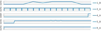
6.3
CPU utilization
In Figure 13, the number of active threads is shown over time when searching CITIES-LARGE. The graphs of 1 A, 4 B, 5 C, and 5 D are not shown since they are very similar to 1 B, 4 A, 5 B, and 5 B, respectively. Most of the programs start preprocessing with one thread and then increase the number of threads. Program 3 A is the only program which does not follow this pattern. Load scheduling of programs 1 B and 4 A can possibly be improved, since these programs do not make constant use of the full number of available cores. Program 4 A has a long single-thread preprocessing phase; queries are answered using 16 threads.
In Figure 14, the number of active threads is shown
over time when joining READS-MEDIUM withk= 4.
The graphs of 1 A, 4 B, 5 C, and 5 D are not shown since they are very similar to 1 B, 4 A, 5 B, and 5 B, respectively. The overall join time for 1 B is only few seconds, so the graph is not as stable as the other ones. For Program 4 A and 5 B the preprocessing phase can be clearly identified (with only one thread). Program 4 A makes use of 16 threads again instead of only 8. Program 9 A uses 8 threads for most of the time. (only the first few seconds are run with only one thread).
6.4
Redundancy
The official rules allowed to serialize the same answer several times: sometimes the same result is found by dif-ferent components of a search algorithm independently. In Figure 26, we analyze the redundancy in the results. The programs of Team 4 and Team 5 report answers
several times (in average 4-6 times). All other programs report each answer only once (baseline 100 percent).
7.
CONCLUSION
We believe that our evaluation gives a fairly represen-tative picture of the state-of-the-art in string similarity search and join for different data set sizes, different al-phabet sizes, and different error thresholds.. Based on our datasets and competing programs, we conclude that an error rate of 20-25% pushes today’s techniques to the limit. For instance, self-joining a set of 15.000.000 se-quence reads of length 100 with an edit distance
thresh-old k = 16 takes almost one day even for the best
participant. However, the final result has more than 50.000.000 entries, which makes the usefulness of such queries in real applications questionable.
Our experiments showed that many participants used
less main memory than available. The effect is
per-spicuous for our CITIES dataset: more than half of the competitors used less than 10 percent of the main mem-ory. An interesting lead for future research are indexing strategies that make full use of existing main memory. Even for smaller datasets, query answering times might be further reduced by more precomputation at indexing time.
Although we have ranked programs based on search time, we have also measured indexing time separately. We found that indexing times vary a lot between im-plementations; in addition many programs use only one thread for indexing. Another point that could be im-proved as revealed by our analysis is to improve thread utilization, especially for current hardware with their quickly increasing number of cores.
It is interesting to note that the three top perform-ing teams use difference techniques. Combinperform-ing these techniques, e.g. the bit-parallel LCS computation from Team 3 with the pruning techniques of Team 1, could probably reduce search and join times beyond the state-of-the-art.
8.
ACKNOWLEDGMENTS
We thank Nikolaus Augsten for his insightful comments on a draft version of this paper. In addition, we thank Thomas Stoltmann for providing us Figure 1.
9.
REFERENCES
[1] A. Arasu, V. Ganti, and R. Kaushik. Efficient
exact set-similarity joins. InPVLDB, VLDB ’06,
pages 918–929. VLDB Endowment, 2006. [2] R. J. Bayardo, Y. Ma, and R. Srikant. Scaling up
all pairs similarity search. InProceedings of the
16th international conference on World Wide
Web, WWW ’07, pages 131–140, New York, NY,
USA, 2007. ACM.
[3] A. Behm, R. Vernica, S. Alsubaiee, S. Ji, J. Lu, L. Jin, Y. Lu, and C. Li. UCI Flamingo Package 4.1, 2010.
[image:11.612.83.287.266.330.2][5] P. Ciaccia, M. Patella, and P. Zezula. M-tree: An efficient access method for similarity search in
metric spaces. InPVLDB, VLDB ’97, pages
426–435, San Francisco, CA, USA, 1997. Morgan Kaufmann Publishers Inc.
[6] M. Crochemore, C. S. Iliopoulos, Y. J. Pinzon, and J. F. Reid. A fast and practical bit-vector algorithm for the Longest Common Subsequence
problem.Information Processing Letters, 80(6),
Dec. 2001.
[7] D. Dey, S. Sarkar, and P. De. A distance-based approach to entity reconciliation in heterogeneous
databases.IEEE Trans. Knowl. Data Eng.,
14(3):567–582, 2002.
[8] J. Feng, J. Wang, and G. Li. Trie-join: a trie-based method for efficient string similarity
joins.The VLDB Journal, 21(4):437–461, 2012.
[9] D. Fenz, D. Lange, A. Rheinl¨ander, F. Naumann,
and U. Leser. Efficient similarity search in very large string sets. In A. Ailamaki and S. Bowers,
editors,Scientific and Statistical Database
Management, volume 7338 ofLecture Notes in
Computer Science, pages 262–279. Springer Berlin
Heidelberg, 2012.
[10] X. Ge and P. Smyth. Deformable Markov model templates for time-series pattern matching. In
Proceedings of SIGKDD, pages 81–90, New York,
NY, USA, 2000. ACM.
[11] S. Gerdjikov, S. Mihov, P. Mitankin, and K. U. Schulz. Good parts first - a new algorithm for approximate search in lexica and string databases.
ArXiv e-prints, Jan. 2013.
[12] A. Gionis, P. Indyk, and R. Motwani. Similarity
search in high dimensions via hashing. InPVLDB,
VLDB ’99, pages 518–529, San Francisco, CA, USA, 1999. Morgan Kaufmann Publishers Inc. [13] M. Henzinger. Finding near-duplicate web pages:
a large-scale evaluation of algorithms. SIGIR ’06, pages 284–291, New York, NY, USA, 2006. ACM.
[14] H. Hyyr¨o, K. Fredriksson, and G. Navarro.
Increased bit-parallelism for approximate and
multiple string matching.ACM Journal of
Experimental Algorithmics, 10, 2005.
[15] G. Li, D. Deng, J. Wang, and J. Feng. Pass-join: A partition-based method for similarity joins.
PVLDB, 5(3):253–264, 2011.
[16] H. Li and R. Durbin. Fast and accurate short read alignment with Burrows-Wheeler transform.
Bioinformatics (Oxford, England),
25(14):1754–1760, 2009.
[17] Y. Li, A. Terrell, and J. M. Patel. WHAM: a high-throughput sequence alignment method. SIGMOD ’11, pages 445–456. ACM, 2011. [18] S. Mihov and K. U. Schulz. Fast approximate
search in large dictionaries.Computational
Linguistics, 30(4):451–477, 2004.
[19] P. Mitankin, S. Mihov, and K. U. Schulz. Deciding word neighborhood with universal
neighborhood automata.Theoretical Computer
Science, 412(22):2340 – 2355, 2011.
[20] I. Moraru and D. G. Andersen. Exact pattern
matching with feed-forward Bloom filters.J. Exp.
Algorithmics, 17(1):3.4:3.1–3.4:3.18, Sept. 2012.
[21] G. Navarro and R. Baeza-Yates. A hybrid
indexing method for approximate string matching.
Journal of Discrete Algorithms, 1(1):205–239,
2000.
[22] M. Patil, S. V. Thankachan, R. Shah, W.-K. Hon, J. S. Vitter, and S. Chandrasekaran. Inverted
indexes for phrases and strings. InSIGIR 2011,
pages 555–564, 2011.
[23] A. Rheinl¨ander and U. Leser. Scalable sequence
similarity search and join in main memory on
multi-cores. InProceedings of the 2011
international conference on Parallel Processing
-Volume 2, Euro-Par’11, pages 13–22, Berlin,
Heidelberg, 2012. Springer-Verlag.
[24] E. Siragusa, D. Weese, and K. Reinert. Fast and accurate read mapping with approximate seeds
and multiple backtracking.Nucleic acids research,
Jan. 2013.
[25] B. S. T. Bocek, E. Hunt. Fast Similarity Search in Large Dictionaries. Technical Report ifi-2007.02, April 2007. http://fastss.csg.uzh.ch/.
[26] A. Tiskin. Semi-local longest common
subsequences in subquadratic time.J. Discrete
Algorithms, 6(4):570–581, 2008.
[27] E. Ukkonen. Algorithms for approximate string
matching.Information Control, 64:100–18, 1985.
[28] G. Wang, B. Wang, X. Yang, and G. Yu. Efficiently indexing large sparse graphs for
similarity search.IEEE Trans. Knowl. Data Eng.,
24(3):440–451, 2012.
[29] W. Wang, C. Xiao, X. Lin, and C. Zhang. Efficient approximate entity extraction with edit distance constraints. SIGMOD ’09, pages 759–770, New York, NY, USA, 2009. ACM.
[30] C. Xiao, J. Qin, W. Wang, Y. Ishikawa, K. Tsuda, and K. Sadakane. Efficient error-tolerant query
autocompletion.PVLDB, 2013.
[31] C. Xiao, W. Wang, and X. Lin. Ed-join: an efficient algorithm for similarity joins with edit
distance constraints.PVLDB, 1(1):933–944, Aug.
2008.
[32] C. Xiao, W. Wang, X. Lin, and J. X. Yu. Efficient similarity joins for near duplicate detection. In Proceedings of the 17th international conference
on World Wide Web, WWW ’08, pages 131–140,
New York, NY, USA, 2008. ACM. [33] C. Xiao, W. Wang, X. Lin, J. X. Yu, and
G. Wang. Efficient similarity joins for
near-duplicate detection.ACM Trans. Database
Prog. 1 100 10,000 100,000 200,000
1_A 199.0000 1.9900 0.0225 0.0042 0.0031
1_B 205.0000 2.0100 0.0220 0.0048 0.0032
2_A - - - -
-3_A 1,625.0000 18.3100 3.0682 4.2107 3.8523
4_A 83.0000 0.7800 0.0101 0.0041 0.0035
4_B 107.0000 0.8700 0.0101 0.0043 0.0030
5_A 50.0000 234.5200 - -
-5_B 52.0000 0.2200 0.0211 0.0160 0.0142
5_C 38.0000 0.1800 0.0228 0.0174 0.0138
5_D 44.0000 0.2100 0.0214 0.0155 0.0144
7_A 116.0000 1.5600 0.5538 0.5519 0.5423
9_A 279.0000 25.7800 24.0174 25.8930 24.8394
[image:13.612.80.289.72.190.2]READS-MEDIUM - Number of queries
Figure 15: Batch effect for READS-MEDIUM:
Time per query for a different number of total queries (1-200,000 queries) [time in milliseconds].
Prog. k=0 k=4 k=8 k=12 k=16
1_A 0.2 0.2 0.3 1.5 25.4
1_B 0.2 0.2 0.4 3.1 42.1
2_A - - - -
-3_A 2.9 30.9 136.2 335.8 972.6
4_A 0.1 0.1 0.4 3.3 17.8
4_B 0.1 0.1 0.4 3.5 20.1
5_A - - - -
-5_B 0.1 0.2 0.9 19.5 56.4
5_C 0.1 0.2 3.9 9.1 108.4
5_D 0.1 0.2 5.2 44.7 160.8
7_A 0.4 5.6 6.4 20.5 30.5
9_A 117.3 242.0 242.5 311.2 1,749.3
MEDIUM
Figure 16: Search times for READS-MEDIUM and
different values ofk[time in seconds].
Prog. k=0 k=1 k=2 k=3 k=4
1_A 0.0 0.0 0.1 0.5 3.5
1_B 0.0 0.0 0.1 0.6 3.0
2_A 8.0 7.0 7.2 16.7 21.3
3_A 5.3 5.2 5.5 6.0 8.0
4_A 0.0 0.0 0.1 0.9 6.2
4_B 0.0 0.0 0.2 0.9 5.9
5_A 178.4 172.8 154.3 159.9 194.7
5_B 0.0 0.6 6.2 63.3 206.1
5_C 0.0 0.7 9.2 39.1 199.1
5_D 13.6 11.9 24.6 58.4 119.0
6_A 0.3 2.3 5.4 7.8 15.4
8_A 0.1 0.1 0.6 4.0 18.4
9_A 0.0 0.1 0.3 2.5 9.1
[image:13.612.317.557.72.196.2]MEDIUM
Figure 17: Search times for CITIES-MEDIUM [time in seconds].
Prog. TINY SMALL MEDIUM LARGE HUGE
1_A 0.5 1.1 1.6 4.4 9.6
1_B 0.5 0.6 1.8 4.6 9.9
3_A 2.0 8.3 200.3 1,836.1 15,531.2
4_A 2.5 29.8 288.5 870.0 2,258.0
4_B 2.0 23.8 234.5 709.9 1,764.5
5_A 19.5 1,813.8 - -
-5_B 2.5 3.3 5.2 9.5 30.8
5_C 2.5 3.3 4.7 9.2 30.9
5_D 2.5 4.0 5.1 9.2 30.6
9_A 0.5 1.2 7.0 9.1 328.7
[image:13.612.319.555.238.355.2]READS k=0
Figure 18: Join times for READS andk= 0 [time
in seconds].
Prog. TINY SMALL MEDIUM LARGE HUGE
1_A 0.7 3.0 10.5 117.0 345.5
1_B 0.9 3.0 11.0 119.5 353.0 3_A 6.5 31.0 68.5 577.0 1,700.0 4_A 2.0 17.0 54.0 807.0 945.0 4_B 2.5 17.0 57.5 810.0 942.0
5_A 10.4 205.5 982.5 -
-5_B 13.8 241.0 920.5 -
-5_C 15.0 226.5 926.0 -
-5_D 22.6 266.0 838.5 2,401.0 -8_A 6.0 141.5 532.5 3,585.0 21,230.0
9_A 16.1 193.5 578.5 -
-CITIES k=4
Figure 19: Join times for CITIES and k=4 [time in seconds].
Prog. TINY SMALL MEDIUM LARGE HUGE 1_A 0.5 9.8 1,028.3 11,283.9 82,636.5 1_B 0.5 26.0 2,941.0 33,055.5
-3_A 26.0 1,732.3 - -
-4_A 33.1 362.8 4,048.4 25,823.9 149,344.1
4_B 32.5 361.7 - -
-5_A 19.8 2,217.3 - -
-5_B 4.1 50.8 4,200.9 -
-5_C 31.0 431.0 - -
-5_D 40.0 625.0 - -
-9_A 159.7 9,327.3 - -
-READS k=16
Figure 20: Join times for READS andk= 16 [time
in seconds].
Threads Progr. k=0 k=4 k=8 k=12 k=16 1_A 1.22 8.51 16.22 87.95 1,000.14 4_A 460.37 470.45 633.01 1,724.68 6,077.06 5_B 3.04 80.29 213.45 3,538.78 10,230.97 1_A 1.23 6.76 10.76 33.96 381.07 4_A 460.26 462.56 576.99 869.19 2,354.78 5_B 5.63 55.41 162.01 3,679.70 9,808.58 1_A 1.22 6.64 9.57 23.61 335.73 4_A 469.87 460.93 486.23 645.42 1,318.72 5_B 3.76 52.55 188.61 3,437.48 5,157.10 8
24
80
[image:13.612.80.289.242.357.2]READS-MEDIUM
Figure 21: Join times for READS-MEDIUM on Sys-tem 2 [time in seconds].
Prog. TINY SMALL MEDIUM LARGE HUGE
1_A 0.6 0.6 0.6 0.6 1.0
1_B 0.8 0.7 0.7 0.6 1.1
3_A 5.8 28.4 56.7 287.2 588.1
4_A 1.9 4.2 7.0 24.9 40.9
4_B 1.7 4.3 7.2 25.0 39.7
5_A 7.7 175.1 850.1 -
-5_B 4.7 4.6 4.5 6.7 11.3
5_C 4.6 4.7 4.8 6.3 11.3
5_D 4.9 4.8 4.8 6.2 11.4
8_A 1.0 0.6 0.9 1.4 3.3
9_A 0.7 1.0 0.6 3.4 10.9
[image:13.612.320.555.394.505.2]CITIES k=0
[image:13.612.80.286.400.523.2] [image:13.612.317.556.536.665.2] [image:13.612.80.289.564.664.2]Threads Progr. k=0 k=1 k=2 k=3 k=4 1_A 0.06 0.30 0.53 1.83 8.12 4_A 10.40 10.35 11.15 17.06 46.00 5_B 1.45 4.17 56.12 376.39 2,513.64 1_A 0.08 0.27 0.38 0.94 3.14 4_A 10.42 10.37 10.69 12.60 22.76 5_B 5.76 4.07 65.28 760.71 2,353.97 1_A 0.11 0.31 0.39 0.85 2.42 4_A 10.47 10.46 10.48 11.37 16.76 5_B 2.38 3.92 42.47 532.91 2,051.15 24
80
CITIES-MEDIUM
[image:14.612.74.310.87.190.2]8
Figure 23: Join times for CITIES-MEDIUM on Sys-tem 2 [time in seconds].
0.0 10.0 20.0 30.0 40.0 50.0
1_A 1_B 3_A 4_A 4_B 5_B 5_C 5_D 7_A 9_A
Memory
[image:14.612.71.311.256.320.2](GB)
Figure 24: Peak main memory usage for READS-HUGE [memory in GB].
0.1 1 10 100
1_A 1_B 3_A 4_A 4_B 5_B 5_C 5_D 6_A 8_A 9_A
Memory
(GB)
Figure 25: Peak main memory usage for CITIES-HUGE [memory in GB].
Prog. 1 100 10,000 100,000 200,000 1_A 100.0% 100.0% 100.0% 100.0% 100.0% 1_B 100.0% 100.0% 100.0% 100.0% 100.0%
2_A - - - -
-3_A 100.0% 100.0% 100.0% 100.0% 100.0% 4_A 100.0% 200.0% 645.8% 479.2% 609.1% 4_B 100.0% 200.0% 645.8% 479.2% 609.1% 5_A 100.0% 200.0% 445.8% 479.8% 465.7% 5_B 100.0% 200.0% 445.8% 479.8% 465.7% 5_C 100.0% 200.0% 445.8% 479.8% 465.7% 5_D 100.0% 200.0% 445.8% 479.8% 465.7% 7_A 100.0% 100.0% 100.0% 100.0% 100.0% 9_A 100.0% 100.0% 100.0% 100.0% 100.0%
READS-MEDIUM - Number of queries
[image:14.612.74.296.386.447.2] [image:14.612.74.310.509.645.2]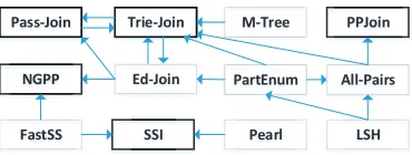

![Figure 5: Search times for READS on System 2[time in seconds].](https://thumb-us.123doks.com/thumbv2/123dok_us/9549009.459749/8.612.325.534.213.342/figure-search-times-reads-time-seconds.webp)
![Figure 7:Search times for CITIES on System 2[time in seconds].](https://thumb-us.123doks.com/thumbv2/123dok_us/9549009.459749/9.612.81.288.72.152/figure-search-times-cities-time-seconds.webp)
![Figure 12: Indexing and Search times for Flamingo,Pearl, and SSI [time in seconds].](https://thumb-us.123doks.com/thumbv2/123dok_us/9549009.459749/10.612.326.531.210.265/figure-indexing-search-times-flamingo-pearl-ssi-seconds.webp)
![Figure 22: Join times for CITIES and k=0 [time inseconds].](https://thumb-us.123doks.com/thumbv2/123dok_us/9549009.459749/13.612.320.555.394.505/figure-join-times-cities-k-time-inseconds.webp)
![Figure 26: Result redundancy: Searching READS-MEDIUM with k=4 for different number of queries(1-200,000) [redundancy in percent; 100% stands forno redundant results; 200% means that in averageeach result is reported twice].](https://thumb-us.123doks.com/thumbv2/123dok_us/9549009.459749/14.612.74.310.87.190/figure-redundancy-searching-dierent-redundancy-redundant-averageeach-reported.webp)
