Manifold learning for the emulation of spatial fields from computational models

warwick.ac.uk/lib-publications

Original citation:

Xing, W. W, Triantafyllidis, V, Shah, A. A., Nair, P. B. and Zabaras , Nicholas. (2016) Manifold

learning for the emulation of spatial fields from computational models. Journal of

Computational Physics, 326. 666 - 690.

Permanent WRAP URL:

http://wrap.warwick.ac.uk/85674

Copyright and reuse:

The Warwick Research Archive Portal (WRAP) makes this work by researchers of the

University of Warwick available open access under the following conditions. Copyright ©

and all moral rights to the version of the paper presented here belong to the individual

author(s) and/or other copyright owners. To the extent reasonable and practicable the

material made available in WRAP has been checked for eligibility before being made

available.

Copies of full items can be used for personal research or study, educational, or not-for-profit

purposes without prior permission or charge. Provided that the authors, title and full

bibliographic details are credited, a hyperlink and/or URL is given for the original metadata

page and the content is not changed in any way.

Publisher’s statement:

© 2016, Elsevier. Licensed under the Creative Commons

Attribution-NonCommercial-NoDerivatives 4.0 International http://creativecommons.org/licenses/by-nc-nd/4.0/

A note on versions:

The version presented here may differ from the published version or, version of record, if

you wish to cite this item you are advised to consult the publisher’s version. Please see the

‘permanent WRAP URL’ above for details on accessing the published version and note that

access may require a subscription.

from computational models

W.W. Xinga_{, V. Triantafyllidis}a_{, A.A. Shah}a,∗_{, P.B. Nair}b_{, N. Zabaras}c,a a_{Warwick Centre for Predictive Modelling, University of Warwick, Coventry CV4 7AL, UK}

b_{University of Toronto Institute for Aerospace Studies, 4925 Dufferin Street, Toronto,} Ontario, Canada M3H 5T6

c_{Department of Aerospace and Mechanical Engineering, University of Notre Dame, 365}

Fitzpatrick Hall of Engineering, Notre Dame, IN 46556-5637, USA

Abstract

Repeated evaluations of expensive computer models in applications such as de-sign optimization and uncertainty quantification can be computationally infea-sible. For partial differential equation (PDE) models, the outputs of interest are often spatial fields leading to high-dimensional output spaces. Although emu-lators can be used to find faithful and computationally inexpensive approxima-tions of computer models, there are few methods for handling high-dimensional output spaces. For Gaussian process (GP) emulation, approximations of the correlation structure and/or dimensionality reduction are necessary. Linear di-mensionality reduction will fail when the output space is not well approximated by a linear subspace of the ambient space in which it lies. Manifold learning can overcome the limitations of linear methods if an accurate inverse map is available. In this paper, we use kernel PCA and diffusion maps to construct GP emulators for very high-dimensional output spaces arising from PDE model simulations. For diffusion maps we develop a new inverse map approximation. Several examples are presented to demonstrate the accuracy of our approach.

Keywords: Parameterized partial differential equations, Gaussian process emulation, High dimensionality, Manifold learning, Inverse mapping, Kernel PCA, Diffusion maps

1. Introduction

An emulator (or surrogate model) is an approximation of a high-fidelity compu-tational model (simulator) that is employed in cases where use of the simulator is computationally impractical or simply infeasible [1, 2]. Applications include un-certainty quantification, design optimization and inverse parameter estimation, which demand repeated simulations in an input parameter space [3, 4]. Statisti-cal (data-driven) emulators are based on supervised machine learning methods, notably polynomial response surface models, Gaussian process models and arti-ficial neural networks, which are applied to input-output data generated by the simulator at judiciously selected design points [2].

In this paper, we are concerned with the emulation of outputs invery high-dimensional spaces, motivated by the problem of emulating spatial fields (e.g., velocity, temperature, electric) fromparameterized partial differential equation (PDE) models. The dimensionality of the output space in this case is equal to the number of points in a spatial grid at which the field variable value is recorded. This number can be very high, especially for problems requiring a fine resolution of the spatial characteristics, e.g., multiple spatial scales or moving boundaries. Emulating such outputs poses unique challenges in terms of the computational cost.

correlation lengths governs all points in the spatial domain. This is essentially the linear model of coregionalization with a so-called intrinsic formulation [13]. Although the resulting method is computationally practical, separability is a severe assumption to make. In many problems of practical interest, e.g., when a phase change takes place, this assumption is invalid. Recent extensions of this idea can be found in [14, 15, 16].

An alternative approach based on dimensionality reduction of the output space was developed by Higdonet al.[17], who used principal component anal-ysis (PCA) combined with separate GPE of the coefficients in the PCA basis. Since the coefficients are uncorrelated, they can be treated as independent, with distinct sets of correlation lengths. A similar approach based on a wavelet de-composition was proposed by Bayarriet al. [18]. As we point out in [19], PCA will fail when the output space does not lie close to a linear subspace of the orig-inal space, e.g., if abrupt changes take place with variations in one or more input parameters. Other linear methods such as independent component analysis and multidimensional scaling suffer from the same issues.

Reduced-order models can also be employed as emulators for PDEs [20, 21, 22, 23]. The approach in this case is typically based on projecting the original PDE system onto a reduced-dimensional subspace obtained by forward runs of the simulator (snapshots), e.g., via proper orthogonal decomposition (POD). This procedure is combined with a numerical method (typically Galerkin finite element) to approximate the undetermined coefficients, e.g., in a POD basis. Such approaches are attractive since they maintain a direct link to the underly-ing physical principles and provide rigorous estimates of the error [23, 24, 25]. Dealing with nonlinearities, on the other hand, is not straightforward. Moreover, in methods based on weak formulations of the PDEs, affine approximations for the bilinear forms and functionals (in relation to the dependence on parameters) are key to computational efficiency [26].

learn-ing refers to a class of methods that provide low-dimensional representations of data residing in a high-dimensional ambient space [28, 29]. The fundamental assumption is that the data lie on, or close to a manifold of low intrinsic di-mensionality. The development of these methods was motivated by the failure of linear methods such as PCA to handle even relatively simple surfaces such as a swiss roll [28]. They can be categorized in a number of ways, e.g., as ker-nel, embedding, spectral or graphical methods, although these categories are not mutually exclusive [30, 31, 32]. Choosing amongst the methods for a given problem is not straightforward; performance on toy data sets can be misleading and each method requires tuning of free parameters to best approximate the given data set. In the present case, there is, moreover, a strict requirement for the existence of an inverse map from the reduced-dimensional space to the physical ambient space. This excludes the majority of methods, for which no such map, or even approximate map exists.

In this paper, we implement two manifold learning techniques (kernel PCA [33] and diffusion maps [34]) for GPE in high-dimensional spaces, each with their own challenges in terms of constructing a valid basis and finding an inverse map approximation. While a number of inverse map approximations exist for kernel PCA (kPCA), approximations for diffusion maps are limited to low-dimensional embeddings [35]. We outline a new approximation that is computationally effi-cient and stable. Its accuracy on a standard data set is demonstrated before it is used in the main algorithm developed in this paper: the emulation of spatial-field outputs (in high-dimensional spaces) from parameterized PDE models.

2. Statement of the problem

Consider a parameterized nonlinear, system of steady-state PDEs of arbitrary order for dependent variables (scalar fields)ui(x, ξξξ),i= 1, . . . , J, whereξξξ∈Rl

is a vector of parameters and x is the spatial variable. To give a concrete example, theui could refer to velocity components (sayi= 1,2,3) and pressure

(i = 4) in a fluid flow model. The PDEs are permitted to be fully nonlinear and parameterized in an arbitrary fashion (including the initial and boundary conditions). It is assumed that the PDE model is well-posed (solutions exist and are unique) for the range of values ofξξξ considered.

The quantity or quantities of interest can include any or all of the ui, or

functions derived from theui. For the purposes of exposition, consider a single

quantity of interest, denoted simply asu(x;ξξξ). The simulator provides values of u(x;ξξξ) at specified (fixed) locations, x(i), i = 1, . . . , d, on a spatial grid. For different inputsξξξ(j)

∈ Rl, j = 1, . . . , m, the outputs of the simulator can be represented as vectors: y(j) = (u(x(1);ξξξ(j)_{), . . . , u(x}(d)_;ξξξ(j)₎₎T

∈ Rd. This process can be repeated for other spatial fields of interest to derive multiple vectorized outputs inRd. An example of the simultaneous emulation of multiple field outputs is given in Section 7. It is assumed for now that a single outputy (derived from a single scalar fieldu(x;ξξξ)) is the target for emulation.

The simulator can be considered as a mapping ηηη : _{X → M} (assumed to be injective), where _{M ⊂} Rd is the permissible output space and _{X ⊂} Rl is the permissible input space. That is, ηηη(ξξξ) = y = (u(x(1);ξξξ), . . . , u(x(d);ξξξ))T

for an arbitrary inputξξξ. The goal of statistical emulation is to approximate the mapping ηηη given training points y(j) =ηηη(ξξξ(j)₎

∈ M, j = 1, . . . , m. The corresponding inputsξξξ(j)

similar approach is adopted but rather than using PCA coefficients, we place GP priors over coefficients of a reduced-dimensional approximation of points in M, obtained by manifold learning methods. We assume thatM is a smooth manifold in Rd_{. The high dimension d of the output space and the inability}

of linear dimensionality reduction methods such as PCA to capture complex response surfaces is the motivation for our approach.

3. Manifold learning methods

3.1. Kernel principal component analysis

kPCA [33] maps high-dimensional data in a space Mto a higher-dimensional feature spaceF via a mappingφφφ:M →F, in which linear PCA is performed. In our case, the data consists of the training data y(i) _{=ηηη(ξξξ}(i)_{) ∈ M ⊂ R}d_,

i = 1, . . . , m, i.e., simulator outputs at the design pointsξξξ(i) ∈ X ⊂ Rl. The eigen-problem for the sample covariance matrix inF is:

CFw = 1 m

m

X

i=1 e

φ

φφ(y(i))φφeφ(y(i)) T

!

w =λw, (1)

in whichφφφ(e y(i)) =φ(φφ y(i))−φφφ is the i-th centred data point in feature space,

whereφφφ = (1/m)Pm

j=1φφφ(y(j)). The mapping φφφ(·) is implicitly definedvia a

kernel function k(y(i),y(j)) = φφ(φ y(i))T_φφφ(y(j)_{), which generates a kernel} ma-trix K = [Kij] with entries Kij = k(y(i),y(j)). A centred kernel function

e

k(y(i),y(j)) =φφeφ(y(i))Tφφeφ(y(j)) and a centred kernel matrixKe = [Keij] with

en-triesKeij=φφφ(e y(i))Tφφeφ(y(j)) are similarly defined. Note thatKe =HKH, where

H=I₋(1/m)11T is the centering matrix, in whichIis the identity matrix and 1= (1/m)(1, . . . ,1)T ∈ Rm. One of the most widely used kernel functions is the Gaussian kernelk(y(i),y(j)) = exp (_−||y(i)₋y(j)_||2/s2_{), where sis a scale} factor.

Equation (1) shows that the eigenvectorsw are linear combinations ofφφeφ(y(i)),

i.e., w =Pm

i=1αiφφeφ(y(i)). Using this expression in Eq. (1) and premultiplying

byφeφφ(y(i))T (noting thatKe is positive semidefinite), yields the eigenvalue

α

ααi are rescaled byαααi 7→αααi/√λi =αααei. This defines orthonormal eigenvectors e

wi = Pm_j=1αejiφeφφ(y

(j)_{), i = 1, . . . , m, where} e

αji = αji/√λi and αji denote

the j-th components of ααeαi and αααi, respectively. Strictly speaking, there are

min(dimF, m) basis vectorswei, but we assume for the purposes of illustration

that dimF > m, without loss of generality. A mapped training pointφeφφ(y(j))

can be expressed in the basis_{w_ei}mi=1⊂ Fasφφeφ(y(j)) =P

m

i=1zi(y(j))wei, where

thei-th coefficient is calculated as follows:

zi(y(j)) =we

T

iφφeφ(y(j)) =

m

X

l=1 e

αliφeφφ(y(l))Tφφeφ(y(j))

=

m

X

l=1 e

αliKelj=ααeα

T i ekj =αααe

T

iH(kj−K1),

(2)

for i = 1, . . . , m, where kj = (K1j, . . . , Kmj)T and kej = (Ke1j, . . . ,Kemj)T.

We can therefore definez(y(j)) = (z1(y(j)), . . . , zm(y(j)))T, where thezi(y(j)),

i= 1, . . . , m, are given by Eq. (2).

The main properties of PCA carry over to kPCA. With λi < λi−1, i = 2, . . . , m, the variance in the data alongwei(equal toλi) decreases asiincreases

and the coefficients in an expansion of a mapped training point in the basis {wei}

m

i=1 are uncorrelated. The goal is to find an r-dimensional approximation of the points φφφ(e y(j)), where ideally r m. The reconstruction error [36] of

the projectionφφφe_r(y(j)) = P

r

i=1zi(y(j))wei ofφφeφ(y

(j)_{) onto the subspace} Fr =

span(w_e1, . . . ,wer) is given by||φφφer(y (j)₎

−φφeφ(y(j))||2=P

m

i=r+1λ2i, where|| · ||is

the standard Euclidean norm for dimF <_∞or theL2₍

M) norm of (equivalence classes of) square integrable functions on_Mfor dimF =_∞. The value ofris typically chosen according to a variance criterion (or modal energy) [36]: Select rsuch thatPr

i=1λi/Pmi=1λi> %for some threshold%.

We can now define a mappingφφeφ_r:M → Fr as the orthogonal projection of

e

φ

φφ(·) onto{wei}

r i=1:

e

φ φ

φr(y(j)) = r

X

i=1

zi(y(j))wei. (3)

We use the notationzr(y(j)) = (z1(y(j)), . . . , zr(y(j)))T, which, from Eq. (2),

is given byzr(y(j)) = [αααe1. . . ,ααeαr]

T_H(k

for data_{y(i)_}m_i=1. Algorithm 1: kPCA

1: Form a kernel matrixKusing a kernel functionk(·,·):

Centred kernel matrix:Ke ←HKH.

2: Solve eigenvalue problem: Kαeαα=mλααα→(αααi, λi),i= 1, . . . , m,

e α ααi←αααi

√ λi.

3: Selectr < maccording toPr i=1λi/

Pm

i=1λi> %. Then compute:

zi(y(j))←ααeα T

iH(kj−K1) i, j= 1, . . . , m,

zr(y(j))←(z1(y(j)), . . . , zr(y(j)))T j= 1, . . . , m.

Remark 1. We assume that the training data captures the structure of _M sufficiently well to (implicitly) define a representative basis, w_ei, i = 1, . . . , m,

for the imageφeφφ[M]⊂ Fof theentirespaceMunderφφeφ. Equation (3) then yields

a reduced-dimensional approximation φφφe_r(y) =P_ir₌₁z_i(y)w_ei for an arbitrary y _{∈ M}. Equivalently, by the injectivity of y =ηηη(ξξξ), and assuming that the feature map is injective, Eq. (3) defines a map (φφφe_r◦ηηη)(·) =φφφe_r(ηηη(·)) :X → Fr,

i.e., directly from theentire permissible input spaceX toFr. The basis vectors

are, however, unknown without an explicit form forφφφ. For an arbitrary input ξξξ ∈ X, the coefficientszi(y) define computable maps zi(·) =zi(ηηη(·)) :X →R

andzr(ηηη(·)) :X →Rr. Thus:

e

φφφr(ηηη(ξξξ)) = r

X

i=1

zi(ξξξ)wei,

zr(ηηη(ξξξ)) = (z1(ξξξ), . . . ,zr(ξξξ))T.

(4)

The original problem of approximatingηηη : _{X → M} given the training points {y(j)_}m_j=1 is replaced by the problem of approximatingzr(ηηη(·)).

A multivariate GP prior indexed byξξξ is placed over zr(ηηη(·)). Algorithm 1

applied to the original training set{y(i)_}m_i=1 yields the new training points for emulation: zr(ηηη(ξξξ(j))) =zr(y(j)) = [αααe1. . . ,ααeαr]

T_H(k

3.2. Diffusion maps

In diffusion maps, the training data y(i) _{∈ M ⊂} Rd, i = 1, . . . , m is mapped to a subset ofRm called thediffusion space from which a reduced-dimensional approximation is subsequently obtained [34, 37]. The mapping embeds the data points in diffusion space by preserving adiffusion distance defined between the points in physical space. The data points y(i) are identified with nodes on a graph and a Markov chain is constructed by specifying a measure of ‘connectiv-ity’ (or a ‘kernel’) between the nodes. Consider a weighted undirected graph_G with vertex set_{y(1), . . . ,y(m)_}representing the training points. Edge weights are defined by a symmetric and positive definite kernelk(y(i),y(j)) between the data points, e.g., the Gaussian kernelk(y(i),y(j)) = exp(_−||y(i)₋y(j)_||2/s2_). We assumeG is connected (otherwise the maps can be constructed separately on each connected component).

A diffusion process [38] onGis constructed by normalizing the connectivity (adjacency) matrixK = [Kij], whereKij =k(y(i),y(j)). The degree matrix is

defined asD= diag(d1, . . . , dm), where di =PjKij, and anm×m diffusion matrix is defined byP=D−1K. P= [Pij] is a Markov matrix; the entryPij is

considered to be a transition probabilityp(y(i),y(j)) from nodey(i)toy(j)in a random walk on_G. The correspondingtstep transition probabilitypt(y(i),y(j))

(from y(i) to y(j) in t _∈ N = 1,2, . . . steps) is given by the (i, j)-th entry of Pt=P_{× · · · ×}P.

Since G is connected, P is ergodic and, therefore, possesses a unique sta-tionary distributionπππwith entries πi =di/P_jdj [34]. The symmetric matrix

P0 _{= D}−1/2_KD1/2

possesses the same eigenvalues γ0

i as P. A spectral

de-composition yieldsP0 =SΓΓΓ0ST, where the columns of Sare the orthonormal eigenvectorssi,i= 1, . . . , m, ofP0 and ΓΓΓ0= diag(γ10, . . . , γm0 ). The eigenvalues

are arranged such that 1 = γ0

1 >· · · > γ0m and the eigenvector s1 has entries √_π

i [39]. Phas the spectral decompositionP=QΓΓΓ0Q−1, whereQ=D−1/2S.

The right and left eigenvectors of P are ri = D−1/2si and li = D1/2si,

re-spectively. Thereforel1 =πππ q_P

jdj andr1=1T/ q_P

jdj. The right and left

By the orthogonality of S, Pt =QΓΓΓt_Q−1_{, orP}t ₌ Pm

i=1(γi0)trilTi . The j-th

row vector ofPt, denotedpt_j, is:

pt_j = (pt(y(j),y(1)), . . . , pt(y(j),y(m)))T = m

X

i=1 (γ0

i)trjili, (5)

where rji is the j-th coordinate of ri. ptj can be considered as a probability

mass function, where thei-th entry,i= 1, . . . , m, is the probability of being at nodey(i)aftert steps of a random walk that started at nodey(j).

A diffusion distanceDt(in physical space) is then defined as follows [34]:

Dt(y(i),y(j)) = (pti−ptj)TD−1(pti−ptj)

1/2

. (6)

We can now define a family of diffusion mapsψψψt_:

M → D(t)

⊂Rmbetween the training pointsy(j) and diffusion spaces_D(t)_{as follows [34, 37]:}

ψ

ψψt(y(j)) = (γ10)trj1, . . . ,(γm0 )trjm T

. (7)

The maps are indexed by the free parametert. The coefficients of a mapped pointy(j)are the coefficients ofpt_jin the non-orthogonal basis{li}mi=1. Diffusion maps embed the data points inD(t) _{in the following sense [34, 37, 40]:}

||ψψψt(y(i))₋ψψψt(y(j))_||=Dt(y(i),y(j)), (8)

where _{|| · ||} denotes the standard Euclidean norm. Equation (8) follows from the bi-orthogonality of the left and right eigenvectors. From Eq. (7) and the decay in the eigenvalues, we can define mappingsψψψt

r(y(j)) :M → D

(t)

r ⊂Rr as

follows:

ψψψtr(y(j)) = ((γ10)trj1, . . . ,(γr0)trjr)T, (9)

which give approximations of the training data_{y(j)=ηηη(ξξξ(j)₎ }m

j=1 inRr, where ideallyrm.

In practice, the value of r is usually selected according to a criterion on the eigenvalues, e.g., as the largest index j such that _|(γ0

Algorithm 2: Diffusion maps

1: Form a kernel matrixKusing a kernel functionk(·,·).

Degree of nodei: di←P_jKij i= 1, . . . , m.

Degree matrix: D←diag(d1, . . . , dm).

P0←D−1/2_KD1/2_.

2: Eigenvalue problem: P0s=γs →(si, γi0),i= 1, . . . , m.

ri←D−1/2si and li←D1/2si.

3: Selectras the largest indexjsuch that|(γj0)t|> υ|(γ

0

2)t|for a precisionυ:

ψ ψ ψtr(y

(j)

)←((γ10) t

rj1, . . . ,(γr0) t

rjr)T j= 1, . . . , m.

points decrease since each row ofPtapproaches the stationary distribution (see Eq. (5)). Algorithm 2 summarizes diffusion maps for data_{y(i)_}m_i=1.

In order to develop an inverse map approximation, we generalize diffusion maps to all points inMby taking the limitm→ ∞. In this limit, the random walk on the discrete graph using a Gaussian kernel converges to a discrete-time walk on the continuous state space M [34, 37, 40, 41].Full details of the following are provided in Appendix A. Here we define the key quantities needed to generalize diffusion maps for the analysis that follows in Section 6.2 on the inverse mapping. Letµbe a probability measure on_Mdefining the density of points. In the limitm_{→ ∞}, a one-step transition kernel for the Markov chain on Mcan be defined byp(y0,y) =k(y,y0)/d(y0), from an arbitraryy0 _{∈ M}to an arbitraryy _{∈ M}, whered(y0) = R

Mk(y,y

0_{)dµ(y). A corresponding forward} transfer operator is defined by _Lϕ(y) = R

Mp(y

0_,y)ϕ(y0_)dµ(y0_{) for ϕ(y)} ∈ L2_{(M, µ). This operator is the continuous analogue of multiplication ofPfrom} the left. Thet-step operatorLt_{ϕ=L ◦ L ◦ · · · ◦ Lϕhas a correspondingt-step}

transition kernelpt(y,y0). We can similarly define a backward transfer operator

Rϕ(y) =R

Mp(y,y

0_)ϕ(y0_)dµ(y0_{), which is the analogue of multiplication ofP} from the right.

where γi, ri(y) andli(y) are the (common) eigenvalues and eigenfunctions of

LandR, respectively. They are, respectively, the continuous-space equivalents ofγ0

i, ri and li. Moreover 1 = γ1 > γ2 >· · ·.The key to the inverse map we develop in Section 6.2 is the link between the eigenvalues/eigenvectors ofPand the eigenvalues/eigenfunctions ofLandR.

For a fixedy _{∈ M},pt(y,y0) is the continuous version (a probability density

in y0 _{∈ M}) of the probability mass function defined by Eq. (5); in the latter case, y = y(j) and y0 _{∈ {}y(1), . . . ,y(m)_}, i.e., the finite set of states accessi-ble from y(j).As explained in Appendix A, the j-th components of ri and li

are, respectively, approximations ofri(y(j)) and li(y(j)) based on the training

data. The diffusion distances between any two points y,y0 _{∈ M}are given by Dt = ||pt(y,y0)−pt(y,y0)||1/d, where ||ϕ||21/d =

R

y0_∈M|ϕ(y0)|2/d(y0)dµ(y0) for functions{ϕ: ||ϕ||1/d <∞}. In turn, diffusion mapsψψψt :M → D(t) ⊂`2 are defined on the whole spaceMbyψψψt_{(y) = (γ}t

1r1(y), γ2tr2(y), . . .). Here,`2 denotes the space of sequences{(x1,x2. . .) : P∞j=1x2j <∞}. Truncating the

expansion ofpt at the first r terms leads to r-dimensional approximations of

the diffusion mapsψψψt

r:M → D

(t)

r ⊂Rr, i.e.,ψψψtr(y) = (γ1tr1(y), . . . , γrtrr(y))T.

Given an isotropic kernel k(y,y0), diffusion maps can be generalized by defining a family of anisotropic kernels k(α)(y,y0) = k(y,y0)/(d(y0)α_d(y)α_),

forα_∈R, and normalizing the resulting kernel to generalize p(y0,y) (or Pin

the discrete case) [34, 42, 43]. The standard algorithm described above corre-sponds to the limiting case ofα= 0 (isotropic kernel), and we do not consider anisotropic kernels in this paper due to limited space and the lack of inverse mappings for such special cases. In Section 6.2, we describe a new inverse map for the isotropic case only.

Remark 2. We can instead consider the mappings (ψψψt

r◦ηηη)(·) =ψψψtr(ηηη(·)) :X →

Dr(t) ⊂Rr that map all points in the input space to D(rt). The mapped point

is given by the firstrcoordinates of the transition kernelpt(y,y0) (considering

define composite functionsri(·) =ri(ηηη(·)) :X →Rto obtain:

ψ ψ ψt

r(ηηη(ξξξ)) = (γ1tr1(ξξξ), . . . , γrtrr(ξξξ))T ∈ D(rt). (10)

The original problem of approximating ηηη(_·) is replaced with the problem of approximatingψψψt

r(ηηη(·)) using the empirical eigenvalues γ0i and empirical

eigen-functions (eigenvectors)li andri.

A multivariate GP prior indexed byξξξ is placed overψψψt

r(ηηη(ξξξ)). Algorithm 2

applied to the original data set _{y(i)_}m_i=1 yields the new training points for emulation: ψψψt

r(ηηη(ξξξ(j))) = ψψψr(y(j)) = ((γ01)trj1, . . . ,(γr0)trjr)T, j = 1, . . . , m,

obtained from the empirical eigenfunctions and empirical eigenvalues.

4. Emulation of coefficients in reduced-dimensional approximations

As explained in Remarks 1 and 2, rather than emulating the outputs in _M directly, we place multivariate GP priors over the reduced-dimensional repre-sentations inFrorD(rt). In the actual approach described in Section 5, we place

univariate GP priors over the individual coefficientsri(·) orzi(·) and emulate

these coefficients separately. In this section, we therefore outline scalar GPE. A scalar valued simulator is a functionη:_{X →}Rof inputsξξξ_{∈ X ⊂}Rl. In univariate GPE, a GP prior indexed byξξξ_{∈ X} is placed overη(ξξξ) and the emu-lator is trained using simuemu-lator outputsη(ξξξ(i)_{) at design pointsξξξ}(i)_{. We use the} notationt = (η(ξξξ(1)_{), . . . , η(ξξξ}(m)₎₎T_{. The prior isη(ξξξ)}

|θθθ, βββ_{∼ GP}(m(ξξξ),c(ξξξ, ξξξ0_)), where_GP(m(_·),c(_·,_·)) represents a GP with mean and covariance functionsm(_·) andc(_·,_·), respectively.The most common choices for the mean function are a linear function or a constant. In this work,m ≡0 was assumed by centering the data. θθθ is a vector of hyperparameters (e.g., parameters in the covariance function) that are typically unknowna priori.

Remark 3. A GP noise term can be added to the model, in which caseη(ξξξ) is a latent function while the simulator outputs are the observables: t(ξξξ) = η(ξξξ) +(ξξξ), in which (ξξξ) _{∼ GP}(0, σ2

nδ(ξξξ, ξξξ0)), where δ(·,·) is the Kronecker

for numerical stability. It can be included directly as an additional term in the covariance functionc(ξξξ, ξξξ0_{) (a so called ‘jitter’ or ‘nugget’ [44]), which leads to} the same result for GP priors over the noise and latent function.

We use a square exponential covariance function:

c(ξξξ, ξξξ0_{) =θ}

0exp −(ξξξ−ξξξ0)Tdiag(θ1, . . . , θl)(ξξξ−ξξξ0)+σ2nδ(ξξξ, ξξξ0), (11)

where the last term is the jitter, and setθθθ= (θ0, . . . , θl, σn2)T. The parameters

θ1, . . . , θl are the inverse square correlation lengths. Alternatives to Eq. (11)

include the Mat´ern class of functions and piecewise polynomials, which are also stationary [45].

The conditional predictive distribution at new inputs ξξξ is obtained in a straightforward manner from the joint distributionp(η(ξξξ),t_|θθθ) [45]:

η(·)|t, θθθ∼ GP(m0_{(·;θθθ), ν}0_{(·,·;θθθ)),} m0_{(ξξξ;θθθ) =c(ξξξ)}T_C−1

t and ν0_{(ξξξ, ξξξ}0_{;θθθ) =c(ξξξ, ξξξ}0_{)−c(ξξξ)}T_C−1

c(ξξξ0_), (12) whereC = [Cij] is the covariance matrix with entries Cij =c(ξξξ(i), ξξξ(j)), i, j =

1, . . . , m, and c(ξξξ) = (c(ξξξ(1)_{, ξξξ), . . . ,c(ξξξ}(m)_{, ξξξ))}T_.

The hyperparametersθθθ are unknown. Point estimates [10, 46] such as the maximum likelihood estimate (MLE) are employed in most cases; that is, the predictive distribution is given by Eq. (12) using the MLE estimate. The MLE is given by arg maxθθθR(θθθ), whereR(θθθ) = logp(t|θθθ) is the log likelihood:

R(θθθ) =−1₂ln|C_{| −}1 2t

T_C−1_t

−m₂ ln(2π). (13)

5. Multi-output emulation using manifold learning

We replaced the problem of emulatingηηη:_{X → M}with the problem of emulat-ing the mapzr(ηηη(·)) defined by Eq. (4) or the mapψψψtr(ηηη(·)) defined by Eq. (10).

Multivariate GP priors are placed over these maps, with training points for em-ulation given by Algorithms 1 and 2 for kPCA and diffusion maps, respectively. These multivariate GP priors take a particularly convenient form by assuming independence of the coordinates, as explained below.

The kPCA coefficients, zi(ξξξ), i = 1, . . . , r are mutually uncorrelated;

fol-lowing Higdonet al.[17] (see also the wavelet decomposition approach in [18]) we therefore make the approximation that they arise from independent GPs. The diffusion map coefficientsγiri(ξξξ),i= 1, . . . , r, on the other hand, are not

uncorrelated. As a simplification, however, we treat the underlying GPs as inde-pendent (see Remark 4). For both manifold learning methods, univariate GPE is then performed separately on each coefficient to approximate its value for a new inputξξξ. The process is summarized below for each case, making clear the link between the notation of Sections 3 and 4.

1. kPCA:For a fixedi= 1, . . . , r, we setη(ξξξ) =zi(ξξξ). The training points

are given by Eq. (2): η(ξξξ(j)_{) =z}

i(ξξξ(j)) =ααeα

T

i H(kj−K1), j = 1, . . . , m.

Recall that zi(ξξξ(j)) =zi(ηηη(ξξξ(j))) =zi(y(j)). The expected (mean) value

at an inputξξξ, given by Eq. (12), yields a prediction that is denotedzi(ξξξ)

(to avoid introducing new notation, we do not distinguish betweenzi(ξξξ)

and E[zi(ξξξ)]). We set zr(ηηη(ξξξ)) = (z1(ξξξ), . . . ,zr(ξξξ))T. Again, this is the

expected valueE[zr(ηηη(ξξξ))].

2. Diffusion maps: For a fixed i = 1, . . . , r, we set η(ξξξ) = ri(ξξξ). The

training points are given by Eq. (9): η(ξξξ(j)_{) =r}

i(ξξξ(j)) =rji,j= 1, . . . , m.

Recall thatri(ξξξ(j)) =ri(ηηη(ξξξ)(j))) =ri(y(j)). For a new inputξξξ, Eq. (12)

yields E[ri(ξξξ)], denoted simply as ri(ξξξ). We then obtain (the expected

value of) ψψψt

r(ηηη(ξξξ)) = ((γ10)tri(ξξξ), . . . ,(γr0)trr(ξξξ))T, which approximates

ψψψt

r(ηηη(ξξξ)) = (γ1tri(ξξξ), . . . , γrtrr(ξξξ))T. Note that while the GPE provides

eigenvaluesγi= limm→∞γ0i, which do not depend onξξξ. Thus, theγi0found

from Algorithm 2 are used to compute the predicted value ofψψψt r(ηηη(ξξξ)).

Remark 4. To take account of the correlations between the coefficients when using diffusion maps, the linear model of coregionalization (LMC) [13, 48] could be used to emulate the coefficients simultaneously. Alternatively, the GP model could be replaced by an artificial neural network (ANN). For moderately sized r, neither approach is computationally expensive. In this paper, we compare the

approach of univariate GPs with ANN using Bayesian regularization [49, 50].

To complete the emulation, we must approximate the inverse map from the reduced-dimensional space_Fr or Dr(t) to the physical spaceM ⊂Rd. This

so-called pre-image problem can be solved in a number of ways for kPCA but a stable, computationally efficient solution for diffusion maps in high-dimensional spaces does not exist. In the next section, we provide details of the inverse map approximations for both methods, including a new pre-image solution for diffusion maps. The main algorithm for GPE of outputs in high-dimensional spaces is given in Section 6.3.

Remark 5. The GPE framework furnishes predictive variances, given by Eq. (12). The variances pertain to the coefficients (zi or ri) in an abstract space and

there is no obvious method to translate this information into variances in the predictionsy =ηηη(ξξξ)∈ M. The inverse maps discussed below provide only the predictive means of the pointsy. However, we can derive Monte Carlo (MC) estimates of higher-order statistics for a fixed inputξξξ by drawing samples from the posterior predictive Gaussian distribution (defined by Eq. (12)) over the coefficientsri(y) = ri(ξξξ) or zi(y) = zi(ξξξ) and using the deterministic inverse

maps described below.

6. Inverse mappings: Reconstruction of points in M

The final step is to find approximations of the inverse mappingsφφφ−1

r (·) :Fr→

Mand (ψψψt

r)−1(·) :D

(t)

that these are the inverse mappings for the manifold learning methods (from the reduced dimensional space to physical space) and not the inverse mappings for the composite functions φφφr(ηηη(·)) and ψψψtr(ηηη(·)). In practical terms (since

the feature map is unknown), for kPCA we seek the mapping z−1

r (·) : Rr →

M, or zr 7→ y =ηηη(ξξξ). This can be achieved via a closed-form least-squares

solution [51, 52]. This method, however, can suffer from numerical instabilities ifm < d (number of training points is less than the dimension of _M), as can the fixed-point iterative algorithm of Mika et al. [53] and other minimization routines.

For diffusion maps there has been little progress towards finding an inverse map approximation. Etyngieret al. [35] proposed an optimization procedure designed for 2-d shapes embedded inR3(a closely related method can be found in [54]). This method uses a Delaunay triangulation into r-simplices of the embedded points inDr(t)and takes the points in the simplex containingψψψtr(y) =

ψ

ψψtr(ηηη(ξξξ)) to be the mapped nearestr+ 1 neighbours ofy =ηηη(ξξξ) inM. It then

proceeds to minimize over the pointy and its barycentric coordinates w.r.t. its r+ 1 closest neighbours. For large values of rand d, in particular for dm, this procedure will be highly unstable and computationally expensive.

Given the reduced-dimensional representationzr(y) orψψψtr(y) of an unknown

pointy, a general method for finding the pre-image is to use a weighted average ofNn neighbouring (in some well defined sense) points ofy. The neighbouring

points are taken from the data set, for which the reduced dimensional represen-tations have been computed. In the present case, the data set consists of them training points{y(i)_}m

i=1. The weighted average can be written as follows: y =X

j∈J

ϑ(y(j))y(j), (14)

in which the weightϑ(y(j)) is associated with the data pointy(j),j _{∈ J}, and J ⊆ {1,2, . . . , m_}, which has cardinalityNn, defines the neighbouring points.

For example, the weights can be defined in terms of the distancesdi,∗, between

y and the data pointsy(i),i= 1, . . . , m. The simplest approach, known as local linear interpolation [55, 56] is to takeϑ(y(j)) =d−j,1∗/

Pm

j=1d

−1

the index set_J according to theNnpoints of{y(j)}mi=1with the largest values of ϑ(y(j)). A generalization of this approach uses an isotropic kernel density χ(y,y0) =χ(||y₋y0_||) to weight the samples [57]:

ϑ(y(j)) = χ(y,y (j)₎ Pm

i=1χ(y,y(i))

=Pmχ(dj,∗)

i=1χ(di,∗)

, (15)

The particular form of kernel density used in this paper isχ(y,y0) = exp(_−||y₋ y0_||2), which was found to yield more stable and accurate results than local linear interpolation.

The problem is now reduced to finding the distances di,∗, i = 1, . . . , m, betweeny and the training points y(i). For both manifold learning methods, these distances are calculated by finding the corresponding kernel values and exploiting relationships between the kernel function and distances inM.

6.1. Kernel PCA

The data matrix Φ = [φφφ(y(1)), . . . , φφφ(y(m))] can be centered in feature space byΦ = Φe H, yieldingw_ei=Pmj=1αejiφφeφ(y

(j)_{) =} e

Φαααei= ΦHαααei, where theαααei are

known from Algorithm 1. The uncentered projectionφφφr(y)∈ Fr ofφφφ(e y)∈ F

onto the firstrbasis vectors is given by:

φ φ φr(y) =

r

X

i=1

ziwei+φφφ=

r

X

i=1

ziΦHαααei+ Φ1

= Φ (H[ααα_e1. . . ,ααeαr]zr+1) = Φτττ .

(16)

To find the distances di,∗, we note that the distance dei,∗ betweenφφφ(y(i)) and φ

φφ(y) in F is given by:

e

d2

i,∗=φφφ(y)Tφφφ(y) +φφφ(y(i))Tφ(φφ y(i))−2φφφ(y)Tφφφ(y(i)). (17) Takingφφφ(y)_≈φφφr(y) and substituting Eq. (16) into Eq. (17) yields:

e

d2i,∗≈τττTKτττ+k(y(i),y(i))−2τττTki, (18)

with τττ defined as in Eq. (16). Note that ΦT_{Φ = K and k}

i = ΦTφφφ(y(i)).

e

d2

i,∗= 2−2k(y(i),y), which, equating to the right hand side of Eq. (18), yields k(y(i),y). For the Gaussian kernel, therefore, we obtaind2

i,∗=−s2lnk(y(i),y). Similar relationships exist for other commonly used kernel functions [58], e.g., the polynomial kernelkn(y,y0) = yTy0+c

n

, c∈R, n=N. In combination with Eqs. (14) and (15), the values ofdi,∗yield an approximation ofy =ηηη(ξξξ).

6.2. Diffusion maps

We assume t = 1 (without loss of generality) to simplify the notation. At the practical level, we must work within the finite-dimensional setting in which we now havem+ 1 data points; the training points{y(i)_}m_i=1, and the unknown predictiony =ηηη(ξξξ). The original kernel, degree and Markov matrices (K, D andP) based on the training points can be augmented to reflect the addition of the pointy. The augmented kernel matrix, denotedK, is:

K=





K (k(y(1),y), . . . ,k(y(m),y))T (k(y(1),y), . . . ,k(y(m),y)) k(y,y)



. (19)

The corresponding degree matrix, denotedD, is:

D=



 b

D 0

0 k(y,y) +P

jk(y(j),y)



, (20)

whereDb =D+diag(k(y(1),y), . . . ,k(y(m),y)). The new Markov chain, denoted

P=D−1K, is given by:

P=



 

b

D−1K Db

−1

(k(y(1),y), . . . ,k(y(m),y))T

(k(y(1),y), . . . ,k(y(m),y))

k(y,y) +P

jk(y(j),y)

k(y,y)

k(y,y) +P

jk(y(j),y)



 .

(21) The (m+ 1)-st row vector ofPis denotedp

m+1. Thei-th entry inpm+1 is the transition probability fromy toy(i),i= 1, . . . , m(the last entry is the transition probability fromy toy). From the discussion in Section 3.2 and Appendix A, we know that the i-th entry of p

m+1 approximates (based on the finite set {y(i)_}m_i=1) the value of the transition kernelp(y,y0) =P∞

y =ηηη(ξξξ) fixed, and withy0=y(i); the last entry is the value aty0=y. Thus:

p

m+1 ≈

∞

X

j=1

γjrj(y)(lj(y(1)), . . . , lj(y(m)), lj(y))T

≈

r

X

j=1

γjrj(y)(lj(y(1)), . . . , lj(y(m)), lj(y))T,

(22)

by virtue of the decay inγi. The value oflj(y(i)),i= 1, . . . , m, is approximated

by thei-th componentlij of lj (the empirical eigenfunction obtained from the

training points). The predicted diffusion coordinates satisfy:

ψ

ψψr(y) = (γ10r1(ξξξ), . . . , γr0rr(ξξξ))T = (γ10r1(y), . . . , γr0rr(y))T. (23)

Recall thatri(ξξξ) =ri(ηηη(ξξξ)), which is numerically equal tori(y) fori= 1, . . . , r,

and is thus known. Thus thei-th entry p_m+1,i of p

m+1 can be approximated as follows:

p_m+1,i≈

r

X

j=1

γ0jrj(ξξξ)lij, i= 1, . . . , m. (24)

Equating this expression with that of the equivalent entry in Eq. (21), we obtain the following:

r

X

j=1

γj0rj(ξξξ)lij=

k(y(i),y)

k(y,y) +Pm

j=1k(y(j),y)

, i= 1, . . . , m. (25)

For a Gaussian kernel k(y,y) = 1, so solving the system of m equations above yields the unknown kernel valuesk(y(i),y),i= 1, . . . , m. The Euclidean distances di,∗ are recovered from the kernel values. For a Gaussian kernel, d2

i,∗=−s2lnk(y(i),y). In combination with Eqs. (14) and (15), these values of di,∗ yield an approximation ofy =ηηη(ξξξ).

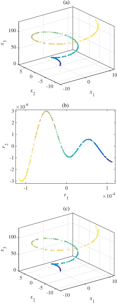
The results of this inverse map approximation on a conical spiral are illus-trated in Fig. 1. A conical spiral is a 1-d manifold embedded in 3-d, and is defined by the following equations:

x1= 4πtcos(4πt), x2= 4πtsin(4πt), x3= 40πt, (26)

0

5 50

x

3

10 0

(a)

100

x

2 x

1

-5 0

-10 _-10

-1 0 1

r₁ ×10-4

-3 -2 -1 0 1 2 3

r

2

×10-6 (b)

0

5 50

x

3

10 0

(c)

100

x

2 x

1

-5 0

-10 _-10

Figure 1(a) shows the sampled points, Fig. 1(b) shows the 2-d (r= 2) approxi-mation of the points using diffusion maps, and Fig. 1(c) shows the reconstruction of the original points using the inverse mapping described above. Here, we used t= 1 and a Gaussian kernel with s2 _{given by the average square distance} be-tween observations in the original space [59], as detailed in Section 7.1. Similarly accurate results were obtained for other standard test sets, e.g., the swiss roll and a Gaussian surface.

6.3. Main algorithm

Algorithm 3: GPE for high-dimensional spaces using manifold learning.

1: Manifold Learning for reduced-dimensional space approximation

kPCA Diffusion maps

Algorithm 1: Algorithm 2:

n

(z1(y(j)_{), . . . , z}

r(y(j)))T om

j=1

(γ10rj1, . . . , γ0rrjr)T m j=1

zi(ηηη(ξξξ(j)))←zi(y(j)) ri(ηηη(ξξξ(j)))←ri(y(j))←rji

2: fori←1 tordo

kPCA Diffusion maps

n

zi(ξξξ(j))←zi(ηηη(ξξξ(j))) om

j=1

n

ri(ξξξ(j))←ri(ηηη(ξξξ(j))) om

j=1 n

η(ξξξ(j)_)←z i(ξξξ(j))

om

j=1

n

η(ξξξ(j)_)←r i(ξξξ(j))

om

j=1

Scalar GPE:zi(ξξξ)←E[η(ξξξ)] Scalar GPE:ri(ξξξ)←E[η(ξξξ)]

3: end for

kPCA Diffusion maps

zr(ηηη(ξξξ))←(z1(ξξξ), . . . ,zr(ξξξ))T ψψψrt(ηηη(ξξξ))←(γ1tri(ξξξ), . . . , γtrrr(ξξξ))T

4: Inverse map

y← Nn X

i=1

χ(di,∗) PNn

i=1χ(di,∗) !

y(i)

kPCA Diffusion maps (t= 1)

k(y(i),y)← 1 2 1−τττ

T

Kτττ+ 2τττTki

r X

j=1

γj0rj(ξξξ)lij←

k(y(i)_,y)

1 +Pm

j=1k(y(j),y) di,∗←

p

−s2_lnk(y(i)_{,y) d} i,∗←

p

−s2_lnk(y(i)_,y)

7. Results and discussion

simulations were performed to yield data pointsy(i)=ηηη(ξξξ(i)₎

∈Rd. Of the 500 data points, mt = 300 were reserved for testing and the training points were

selected from the remaining 200 (m≤200). We usey(pi)=ηηη(ξξξ(i)) to denote the

predicted value ofy(i)_{at a test inputξξξ}(i)_{,i= 1, . . . , m}

tusing Algorithm 3. A

relative error is defined as:

Relative error =||y (i)

p −y(i)||2

||y(i)_||2 , (27)

where_{|| · ||}is the standard Euclidean norm.

7.1. Computational details

Details of the scalar GPE, the manifold learning techniques and the software employed in the implementation of Algorithm 3 are provided below.

1. kPCA.A Gaussian kernel was used with the free parameters2_{taken to be} the average square distance between observations in the original space [59]: s2 _{= (1/m}2₎Pm

i,j=1||y(i)−y(j)||2. Polynomial and multi-quadratic ker-nels were also tested but found to be inferior. A sigmoid kernel was found to give similar results to those obtained with a Gaussian kernel. In the inverse mapping, all m points were employed for the reconstruction in physical space (inverse mapping).

2. Diffusion maps. A Gaussian kernel was used, in which the value of s2 was determined as described above. Again, all m points were employed for the reconstruction. A value oft= 1 was used in the results presented below. Higher values oft did not lead to any significant changes.

7.2. Free convection in porous media

Subsurface flow in a porous medium can be modelled by Brinkman’s equation (with a Boussinesq buoyancy term) and a thermal energy balance [62]:

− ωκ−1v+_∇p

− ∇ ·ω−1 _∇v+_∇vT

=ρgce(T−Tc),

ρCpv· ∇T− ∇ ·(λ∇T) = 0,

∇ ·v = 0,

(28)

in whichv is the flow velocity,T is temperature,pis pressure,g is the gravita-tional acceleration,ρis the fluid density at a reference temperatureTc,andκ

are the porosity and permeability of the medium,ω is the dynamic viscosity,ce

is the coefficient of volumetric thermal expansion,λis the volume averaged ther-mal conductivity of the fluid-solid mixture, andCpis the specific heat capacity

of the fluid at constant pressure.

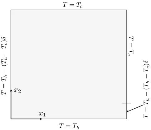
We consider a 2-d domain (x1, x2)∈[0,10]×[0,10] (in cm) filled with water. The temperature boundary conditions are illustrated in Fig. 2. The temperature ranges from Th to Tc < Th along the outer edges. Buoyant flow is generated

by the nonuniform temperature. No-slip conditions on all boundaries (with an arbitrary reference p) are assumed. The model was solved using the finite element method (FEM) with triangular elements and a quadratic Lagrange nodal basis. Details of the implementation and default parameter values can be found in [63].

Training and Testing. In this example, the input parameters were ξξξ = (ce[K−1], Th[oC])T ∈[10−11,10−8]×[40,60]. For each inputξξξ(i),i= 1, . . . ,500,

the magnitude_|v_|of the velocity was recorded at each grid point on a regular 100_×100 square spatial grid and the d= 104 _{values of}

|v_| were vectorized to yield the data points y(i) _∈ Rd, i = 1, . . . ,500. In the notation of Section 2, u(x;ξξξ) =_|v_|,J = 1,l= 2 andd= 104_.

T =Tc

T =Th

T

=

T

c

T

=

Th

−

(

Th

−

Tc

)

δ

T

=

Th

−

(

Th

−

Tc

)

δ

x

x

Figure 2: Temperature boundary conditions for the free-convection example. δis a variable that represents the relative length of a boundary segment and goes from 0 to 1 along the segment as x2 increases. The cut-off shown by the horizontal dash along x1 = 10 cm is

located atx2= 1 cm.

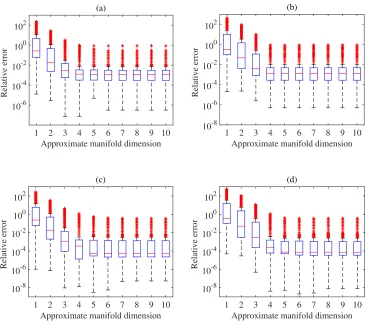
and upper lines (whiskers) define the errors within 1.5×(Q3−Q1) of the first and third quartiles. All other points (considered outliers) are plotted individually using a ‘+’ symbol. A decrease in the relative error for an increasingris seen for both kPCA and diffusion maps. For both methods, the errors converge at around r = 6 dimensions. The median value of the error is marginally lower with kPCA, but it was found that the number of outliers was slightly higher using this method. For a high number of training points (m _≥ 80), both methods provided accurate predictions and the differences in the errors were not significant.A comparison to Higdon’s method [17] can be found in [19], where the same problem is considered and equivalent boxplots are provided. The performance of both kPCA and diffusion maps is far superior. To conserve space, we do not reproduce these results here.

Approximate manifold dimension

1 2 3 4 5 6 7 8 9 10

Relative error

10-6 10-4 10-2 100 102

(a)

Approximate manifold dimension 1 2 3 4 5 6 7 8 9 10

Relative error

10-8 10-6 10-4 10-2 100 102

(b)

Approximate manifold dimension

1 2 3 4 5 6 7 8 9 10

Relative error

10-8 10-6 10-4 10-2 100 102

(c)

Approximate manifold dimension

1 2 3 4 5 6 7 8 9 10

Relative error

10-8 10-6 10-4 10-2 100 102

(d)

Figure 3: Tukey box plots of the relative error||y(pi)−y(i)||2/||y(i)||2in the free-convection

test example (Figs. 4(a)-(c)) lies around the median of the r = 5 boxplot in Fig. 3. The errors with respect to the second test example are close to the upper whiskers in the same boxplots. In both cases, Algorithm 3 with either kPCA or diffusion maps yields highly accurate predictions. An example of the outliers for both methods in the r = 5 boxplots in Figs. 3(c) and 3(d) is shown in Fig. 5. This figure demonstrates the worst level of prediction, which, nevertheless, captures the qualitative features of the velocity field and remains quantitatively accurate to a reasonable level.

Boxplots of the errors using an ANN and support vector machine regression (SVMR) for emulation of the coefficients, rather than GPE, are shown in Fig. 6 form= 120. In the first case, the correlations between the coefficients are nat-urally taken into account by approximating the r coefficients simultaneously. To avoid overtraining and cross validation, Bayesian regularization [49, 50] was used for the ANN, implemented in the Matlab Neural Network Toolbox. In this method, zero-mean Gaussian priors are placed over the network weights and an additive noise. Estimates of the weights and hyperparameters (variances in the priors) are found by an iterative procedure based on a Laplace approximation to the posterior over the weights and an evidence approximation for the hyperpa-rameters [47]. A single hidden layer was employed and the number of neurons was selected using a sequential network construction [50].For the SVMR, we tested Gaussian and polynomial kernels (with varying order), together with an L1 _{loss function.}

(a)

ξ / cm

20 40 60 80 100

χ / cm 20 40 60 80 100 0.5 1 1.5 2 2.5 3 (d)

ξ / cm

20 40 60 80 100

χ / cm 20 40 60 80 100 0.02 0.04 0.06 0.08 0.1 (b) x 1 / cm

20 40 60 80 100

x 2 / cm 20 40 60 80 100 0.5 1 1.5 2 2.5 3 (e) x

1 / cm

20 40 60 80 100

x 2 / cm 20 40 60 80 100 0.02 0.04 0.06 0.08 0.1 (c) x

1 / cm

20 40 60 80 100

x 2 / cm 20 40 60 80 100 0.5 1 1.5 2 2.5 3 (f) x

1 / cm

20 40 60 80 100

x 2 / cm 20 40 60 80 100 0.02 0.04 0.06 0.08 0.1

Figure 4: Predictions of the velocity field using 120 training points andr = 5 coefficients in the free-convection example. Figure (a) is the test point corresponding toξξξ = (3.18×

10−9_[K−1_],56.7[o_C])T_{, while Figs. (b) and (c) are the corresponding predictions using kPCA}

and diffusion maps, respectively. Figure (d) is the test point corresponding to ξξξ = (7×

(a)

x

1 / cm

20 40 60 80 100

x

2

/ cm

20 40 60 80 100

0.005 0.01 0.015 0.02

(b)

x

1 / cm

20 40 60 80 100

x

2

/ cm

20 40 60 80 100

0.005 0.01 0.015 0.02 0.025 0.03

(c)

x 1 / cm

20 40 60 80 100

x

2

/ cm

20 40 60 80 100

0.005 0.01 0.015 0.02 0.025 0.03

are superior.

7.3. Lid driven cavity

We consider a square 2-d cavity (x1, x2)∈[0,1]×[0,1] filled with liquid water. The top boundary represents a sliding lid, which drives the liquid flow. The problem is governed by the steady-state, dimensionless Navier-Stokes equations:

(v_{· ∇})v₋Re−1 ∇2_v+

∇p= 0, _{∇ ·}v = 0, ₍₂₉₎

wherev = (v1, v2)T is the liquid velocity,pis the liquid pressure andReis the Reynolds number. The boundary conditions arev = (v10,0) forx2= 1, where v0

1 is the lid velocity, andv= 0 on the other three boundaries. The model was solved using finite differencing on a staggered grid with implicit diffusion and a Chorin projection for the pressure [64].

Training and Testing. The Reynold’s number and lid velocity were used as input parameters: ξξξ= (Re, v0

1)T ∈[700,1200]×[0.01,10]. All other parameters were kept at the default values. For each inputξξξ(i)_{,i= 1, . . . ,500, the pressure} pand the component velocitiesv1 andv2were recorded at each grid point on a regular 100×100 spatial grid. Thed/3 = 104 _{values of each field variable were} vectorized to yield vector outputsy(vi1)∈R

d/3_,y(i)

v2 ∈R

d/3 _andy(i)

p ∈Rd/3. The

three vectors were then combined into a single vectory(i)= [y(vi1) y

(i)

v2 y

(i)

p ]∈Rd

to account for the correlations between the fields. In the notation of Section 2, J = 3, l = 2 and d = 3_×104_{. This is a multiple field example discussed in} Section 2, with, e.g.,u1=v1, u2=v2 andu3=p.

1 2 3 4 5 6 7 8 9 10 Approximate manifold dimension 10-8

10-6 10-4 10-2 100 102

Relative error

(a)

1 2 3 4 5 6 7 8 9 10 Approximate manifold dimension 10-8

10-6 10-4 10-2 100 102

Relative error

(b)

1 2 3 4 5 6 7 8 9 10

Approximate manifold dimension 10-10

10-8 10-6 10-4 10-2 100 102

Relative error

(c)

1 2 3 4 5 6 7 8 9 10

Approximate manifold dimension 10-10

10-8 10-6 10-4 10-2 100 102

Relative error

(d)

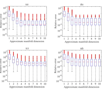
Figure 6: Tukey box plots of the relative error||y(pi)−y(i)||2/||y(i)||2in the free-convection

at the lower number of training points and slightly inferior performance at a higher number of training points.

Two examples of the predictions are shown in Fig. 9 for 120 training points andr= 5. Here, the normalized velocity field is shown as a quiver plot and the surface plot is the pressure field, with contours in black. Note that since only∇p is meaningful, homogeneous Neumann conditions are prescribed for the pressure Poisson equation, so p is defined only up to a constant (hence the negative values). Stream lines representing contour lines of a stream functionζ are also shown, in white. The stream function is defined by_−∇2_ζ=∂

x2v1−∂x1v2. For

both kPCA and diffusion maps, the error with respect to the first test example (Figs. 9(a)-(c)) lies close to the median in ther= 5 boxplot in Fig. 7. The second test example corresponds to an outlier for both methods (relative error around 0.07). The results of Algorithm 3 remain accurate, especially for diffusion maps. The error in kPCA is primarily due to the prediction of the pressure field, in particular the maximum value in the top right corner. Nevertheless, the profile is well captured.

As a further test, we consider a modification of this example, in which the number of inputs is increased to 13 (l = 13) using the following boundary conditions:

v1(x1,1) = 5c1sin(c2πx1)e−c3x1, v2(x1,1) = 0, v1(x1,0) = 5c4sin(c5πx1)e−c6x1, v2(x1,0) = 0, v2(1, x2) = 5c7sin(c8πx2)e−c9x2, v1(1, x2) = 0, v2(0, x2) = 5c10sin(c11πx2)e−c12x2, v1(0, x2) = 0,

(30)

for constants c1, . . . , c12. The inputs were defined as ξξξ = (Re, c1, . . . , c12)T ∈ [500,1000]×(0,1)×(0,1)× · · · ×(0,1). Inputsξξξ(i)_{,i= 1, . . . ,1000 were} gener-ated using a Sobol sequence and simulations were performed to yield 1000 data points. Of the 1000 data points, mt = 300 were reserved for testing and the

Approximate manifold dimension

1 2 3 4 5 6 7 8 9 10

Relative error

10-6 10-4 10-2 100 102 104 106

(a)

Approximate manifold dimension 1 2 3 4 5 6 7 8 9 10

Relative error

10-6 10-4 10-2 100 102 104 106

(b)

Approximate manifold dimension

1 2 3 4 5 6 7 8 9 10

Relative error

10-6 10-4 10-2 100 102 104

(c)

Approximate manifold dimension

1 2 3 4 5 6 7 8 9 10

Relative error

10-6 10-4 10-2 100 102 104

(d)

Figure 7: Tukey box plots of the relative error||y(pi)−y(i)||2/||y(i)||2in the lid-driven cavity

Approximate manifold dimension

1 2 3 4 5 6 7 8 9 10

Relative error

10-6 10-4 10-2 100 102

(a)

Approximate manifold dimension 1 2 3 4 5 6 7 8 9 10

Relative error

10-6 10-4 10-2 100 102

(b)

Figure 8: Tukey box plots of the relative error||y(pi)−y(i)||2/||y(i)||2in the lid-driven cavity

example using Higdon’s method [17] with an increasing approximate manifold dimensionron the 300 test points for: (a) 80 training points; (b) 120 training points.

showing the relative error on the 300 test points for an increasing r (approxi-mate manifold dimension) withm= 500. Two examples of the fields are shown in Fig. 11 using kPCA withr= 10 andm= 500. The first example corresponds to an error near the median (forr= 10) and the second example is an outlier with a large relative error in the corresponding boxplot. As expected, for a higher dimensional input space, more training points are needed to capture the surface _M accurately. In this case, any lower than 400 training points led to poor performance from all methods.

7.4. Hydrogen fuel cell model

In this example, we consider a hydrogen/oxygen polymer electrolyte mem-brane (PEM) fuel cell model that incorporates species conservation, charge con-servation and a momentum balance in the porous layers. The 2-d domain in-cludes the porous gas diffusion layers (GDLs), through which the species (oxy-gen, water and hydrogen) are transported from the channels to the reaction sites in the catalyst layers, which are adjacent to the PEM (Fig. 12).

0 0.2 0.4 x 0.6 0.8 1 1 0 0.2 0.4 0.6 0.8 1 x 2 -2 -1 0 1 2 3 4 5 6 ×10

0 0.2 0.4 x 0.6 0.8 1

1 0 0.2 0.4 0.6 0.8 1 x 2 0 5 10 15 ×10 (b)

0 0.2 0.4 x 0.6 0.8 1

1 0 0.2 0.4 0.6 0.8 1 x 2 -2 -1 0 1 2 3 4 5

×10-3 (e)

0 0.2 0.4 x 0.6 0.8 1

1 0 0.2 0.4 0.6 0.8 1 x 2 -2 0 2 4 6 8 10 12

×10-5

(c)

0 0.2 0.4 x 0.6 0.8 1

1 0 0.2 0.4 0.6 0.8 1 x 2 -2 -1 0 1 2 3 4 5 6

×10-3 (f)

0 0.2 0.4 x 0.6 0.8 1

1 0 0.2 0.4 0.6 0.8 1 x 2 0 5 10 15 ×10-5

Figure 9: Predictions of the velocity field using 120 training points andr= 5 coefficients in the lid driven cavity example. Figure (a) is the test point corresponding toξξξ= (874.8,7.79)T_,

while Figs. (b) and (c) are the corresponding predictions using kPCA and diffusion maps, respectively. Figure (d) is the test point corresponding toξξξ= (773.24,0.77)T_{, while Figs. (e)}

1 2 3 4 5 6 7 8 9 10

Approximate manifold dimension

10-3 10-2 10-1 100

Relative error

(a)

1 2 3 4 5 6 7 8 9 10

Approximate manifold dimension 10-3

10-2 10-1 100

Relative error

(b)

Figure 10: Tukey box plots of the relative error||y(pi)−y(i)||2/||y(i)||2in the lid-driven cavity

example with boundary conditions as in Eq. (30). The trends are shown for an increasing approximate manifold dimensionrusing 600 training points and 300 test points for: (a) kPCA and (b) diffusion maps.

catalyst layer morphology is approximated as clusters (agglomerates) of carbon-supported platinum coated with the electrolyte. The transfer current densities are expressed as follows [66]:

jc=−

12LactF Dagg

R2

agg

CO2,agg(1−mac)(1−λccothλc),

ja =−6LactF Dagg

R2

agg

CH2,agg

1−e−RT2Fηa₍₁₋

mac)(1−λacothλa),

λc =

s

i0cSR2agg

4F CO2,refDagg

e2RTF ηc λ

a=

s

i0aSR2agg

2F CH2,refDagg

,

(31)

where ja(ηa) and jc(ηc) are the anode and cathode transfer current densities

(overpotentials);Ragg andDaggare the radius of the agglomerate and the

dif-fusion coefficient of the reactant through the agglomerate;Lact is the catalyst

layer thickness (same in both half cells); i0a and i0c are the exchange current

densities of the anode and cathode reactions;CO2,ref andCH2,ref are reference

reactant concentrations;CO2,agg andCH2,agg are the (catalyst) surface

(a)

0 0.2 0.4 0.6 0.8 1

x 1 0 0.2 0.4 0.6 0.8 1 x 2 -5 0 5 10 15

×10-3 (c)

0 0.2 0.4 0.6 0.8 1

x 1 0 0.2 0.4 0.6 0.8 1 x 2 0 2 4 6 8 10 12

×10-3

(b)

0 0.2 0.4 0.6 0.8 1

x 1 0 0.2 0.4 0.6 0.8 1 x 2 -5 0 5 10 15

×10-3 (d)

0 0.2 0.4 0.6 0.8 1

x 1 0 0.2 0.4 0.6 0.8 1 x 2 -2 0 2 4 6 8 10 12

×10-3

Figure 11: Predictions of the velocity and pressure fields usingm= 500 training points and

Figure 12: A schematic of the PEM fuel cell and the components that form the model domain.

agglomerate surfaces at a rate governed by Henry’s law, so that:

CH2,agg =pXH2/KH2 CO2,agg=pXO2/KO2, (32)

whereXi(Ki) is the mole fraction (Henry constant) of speciesiandpis the gas

pressure.

The charge balances are given by:

−∇ ·(σe∇φe) = 0 and − ∇ ·(σs∇φs) = 0, (33)

in whichφe(σe) and φs(σs) are the ionic and electronic potentials

(conductiv-ities), respectively. These equations apply to the GDLs. The catalyst layers are approximated by infinitesimally thin surfaces, depicted by∂Ωa and∂Ωc in

Fig. 12. The overpotentials (defined only on these boundaries) take the form:

ηa=φs−φe−Eeq,a and ηc=φs−φe−Eeq,c, (34)

Flow through the GDLs is governed by continuity and Darcy’s law:

∇ ·(ρv) = 0, v=₋kpω−1∇p, (35)

where ω is the gas viscosity and kp is the GDL permeability. The ideal gas

law is used to determine the density: ρ= (p/RT)P

iMiXi, in whichMiis the

molecular weight of species i _{∈ {}H2,O2,H2O,N2}. The transport of species through the GDLs is governed by convection and multicomponent diffusion (Stefan-Maxwell) [67]. In the cathode, the species are _I1 = {O2,H2O,N2} and in the anode the species are_I2={H2,H2O,N2}. The transport equations in the cathode are given by:

−∇ ·

ρYiPj∈I₁

j6=i

Di,j(∇Xj+ (Xj−Yj)∇p/p)

=₋ρv_{· ∇}Yi,

YN2= 1−YO2−YH2O,

(36)

fori_{∈ {}O2,H2O}. Yi is the mass fraction of species iand the Di,j are binary

diffusivities [67]. Identical equations for species_I2are solved in the anode. The boundary conditions for the potential impose a cell voltageVcell:

φs= 0 x ∈∂Ωa,cc,

φs=Vcell x ∈∂Ωc,cc,

−n_{· ∇}φs= 0 otherwise,

(37)

wherenis the outwardly pointing unit normal. At the inlets (∂Ωa,inand∂Ωc,in)

and outlets (∂Ωa,outand∂Ωc,out), the total gas pressures and the mole fractions

of the reactants are specified. At∂Ωa and ∂Ωc, the gas velocity is calculated

from the total mass flow based on Faraday’s law [65]:

−n_·v =ja(MH2/2 +λH2OMH2O)/(ρF) x ∈∂Ωa,

−n_·v =jc(MO2/2 + [1/2 +λH2O]MH2O)/(ρF) x ∈∂Ωc,

(38)

whereλH2O is the water drag number [65]. At the other boundaries except the

mass fluxes of reactants are determined by Faraday’s law: −n_·NH2 =MH2ja/(2F) x ∈∂Ωa,

−n_·NO2=MO2jc/(4F) x ∈∂Ωc,

−n_·NH2O =MH2Ojc(1/2 +λH2O)/F x ∈∂Ωc,

(39)

whereNi=−ρYiPj6=iDi,j(∇Xj+ (Xj−Yj)∇p/p) +ρvYiis the flux of species

i. At all other boundaries except the inlets and outlets, Ni = 0. The model

was solved using the FEM with 10236 triangular domain elements, 582 boundary elements and a Lagrange basis of order 2. Details of the implementation and the default parameter values can be found in [68].

Training and Testing. The cell voltageVcell and the membrane/electrolyte

conductivity σe were used as input parameters: ξξξ = (Vcell[V], σe[S m−1])T ∈

[0.2,0.8]×[1,15]. For each inputξξξ(i)_{,i= 1, . . . ,500, the mole fraction of water} XH2O was recorded at each point on a regular 150×300 spatial grid in the

cathode GDL.XH2Oin the cathode (where water is produced) is a key quantity.

High values can lead to flooding of the electrode, which would prevent the fuel cell from operating. Thed= 4.5_×104_{values ofX}

H2Owere re-ordered into vector

form to yield vectorsy(i)_∈Rd. In the notation of Section 2,u(x;ξξξ) =XH2O,

J = 1,l= 2 andd= 4.5_×104_.

10−7 10−6 10−5 10−4 10−3 10−2

1 2 3 4 5 6 7 8 9 10

Approximate manifold dimension (a)

Relative error

10−7 10−6 10−5 10−4 10−3 10−2

1 2 3 4 5 6 7 8 9 10

Approximate manifold dimension (b)

Relative error

10−8

10−7

10−6

10−5

10−4

10−3

10−2

1 2 3 4 5 6 7 8 9 10

Approximate manifold dimension (c)

Relative error

10−8 10−7 10−6 10−5 10−4 10−3 10−2

1 2 3 4 5 6 7 8 9 10

Approximate manifold dimension (d)

Relative error

Figure 13: Tukey box plots of the relative error||y(pi)−y(i)||2/||y(i)||2 in the PEM fuel cell