Automatic aviation safety reports classification

(1)

1

Faculty of Electrical Engineering,

Mathematics & Computer Science

Automatic aviation

safety reports classification

Andr´es Felipe Torres Cano M.Sc. Thesis

August 2019

Supervisors:

(2)

(3)

Preface

This thesis is dedicated to my family, especially to my parents and future wife.

I want to thank to my supervisors Christin and Maurice for their valuable guidance and feedback. I also extend my gratitude to all the great lecturers that I had at UTwente.

In the same way, thanks to all my colleagues at KLM, to my manager Bertjan and my great friend Arthur.

(4)

(5)

Abstract

In this master thesis we present an approach to automatically classify aviation safety reports by applying supervised machine learning. Our proposed model is able to classify 7 different types of safety reports according to a taxonomy hierarchy of more than 800 labels using a dataset with 19 815 reports which is highly imbalanced. The reports comprise numerical, categorical and text fields that are written in english and dutch languages. Such reports are manually categorized by safety analysts in a multi-label setting. The reports are later aggre-gated according to such taxonomies and reported in dashboards that are used to monitor the safety of the organization and to identify emerging safety issues. Our model trains one classifier per each type of report using a LightGBM base classifier in a binary relevance setting, achieving a final macroaveraged F0.5 score of 50.22%. Additionally, we study the

impact of using different text representation techniques in the problem of classifying aviation safety reports, concluding that term frequency (TF) and term frequency inverse document frequency (TF-IDF) are the best methods for our setting. We also address the imbalanced learning problem by using SMOTE oversampling, improving our classifier performance by 41%. Furthermore, we evaluate the impact of using hierarchical classification in our classi-fier with results suggesting that it does not improve the performance for our task.

Finally, we run an experiment to measure the reliability of the manual classification pro-cess that is carried out by the analysts using Krippendoff’s mvα. We also present some

suggestions to improve such process.

(6)

(7)

Introduction

With approximately 35 000 employees and moving more than 32 million passengers, KLM is one of the leading airlines in Europe. Safety is of vital importance in the aviation industry and it is managed at KLM by the Integrated Safety Management System (ISMS). One of the processes in the ISMS is to collect and analyze safety reports. The reports are reviewed by analysts and categorized with one or more labels that are called taxonomies. Such reports are aggregated according to such taxonomies and reported in dashboards that are used to monitor the safety of the organization and to identify emerging safety issues. Today, the taxonomy classification is done manually and it is the desire of the management that such categorization is performed automatically because it is expected that the number of received reports is going to increase in the following year. Additionally, the management has also expressed concerns about the consistency of the report categorization. There is an impression that the categorization process varies significantly. This means that one report that is categorized today with certain labels would get a slightly different categorization if it is categorized again in one month. Such situation can negatively affect the trust that is given to the aggregated information that is used to monitor the safety of the organization. Therefore, there is a need to check the categorization process and to measure the trust in the data.

This master thesis presents our approach to automatically classify the safety reports by applying supervised machine learning. In the same way, the development of this research delivers important insights about the categorization process and how can it be improved. Firstly, exploratory data analysis (EDA) is used to understand the dataset and to devise the machine learning techniques that can be applied. Secondly, a quick baseline with a logistic regression classifier and a multi-label decision tree is established to serve as a starting point for the automatic classification. Such baseline is used to identify the pre-processing steps that need to be applied to the dataset and to identify the machine learning techniques that will be evaluated. Then, a set of experiments is designed to collect results that support the answers to our research questions. Next, the results of our experiments are analyzed and conclusions are derived.

(10)

1.1 Problem Statement

The main goal of this research is to automatically classify the different safety reports ac-cording to the defined taxonomy. Each taxonomy is a set of labels organized as a hierarchy. There are 7 different types of reports. Each report can be categorized with one or more labels from different taxonomies. The taxonomies that can be applied to each type of report have been established by the company. Due to the business requirements, it is not nec-essary to focus on the zero-shot learning problem, meaning that it is not important to have good performance on labels with a few examples.

The secondary goal is to examine the current data generation process, to measure its reliability and to issue recommendations to improve it.

The main problem can be posed as a multi-label classification task, where N is the

number of instances in the dataset S. Havingxi to be one example and X the set of all

examples, yi is the ordered tuple of labels associated to one example andY the set of all

tuples containing labels. yirepresents one single label andLis the number of unique labels

inY. More formally:

S={(xi,yi)|1≤i≤N,xi⊆X,yi⊆Y}

L=|Y|

yi = (y1, y2, ..., yL), yi ∈ {0,1}

A single taxonomyti= (vi,ei)is a tree that is considered a rooted directed acyclic graph

(DAG) with rootρby definition [1] [2]. All the taxonomies comprise the setTof such graphs:

T={(v1,e1),(v2,e2), ...,(vK,eK)|vi\ {ρi} ∩vj\ {ρj}, i6=j}

vi ={y1,y2, ...,yi|yi⊆Y}

ei={(yi,yj)|yi ⊆Y,yj ⊆Y, i6=j}

After inspecting the taxonomies used to classify the aviation safety reports, we observed that the mentioned taxonomies exhibit the following properties:

• A single label yi only belongs to one taxonomy, meaning that each taxonomy is a

complete independent tree.

• The root of each taxonomy ρ is not considered a label and it is excluded from our

analysis because it can be derived from the report type.

(11)

1.2. RESEARCHQUESTIONS 3

1.2 Research Questions

The proposed approach is to apply supervised machine learning to automatically classify the reports. In order to solve it, we will address the following research questions:

• RQ1: What are the influencing factors on the accuracy of applying supervised machine

learning to classify aviation safety reports automatically? As influencing factors we investigate feature representation and classification model types. More concretely, we want to evaluate what is the impact of using word embeddings over TF-IDF?, what is the impact of using different multi-label learning models? and does hierarchical classification perform better than flat classification?

• RQ2: How can we measure the reliability of the report classification process that is

performed by human analysts? With this question we aim to discover the metric that is more suitable for measuring such reliability.

1.3 Outline

(12)

(13)

Chapter 2

Background

In the following sections we introduce some background concepts. Section 2.1 describes Operational Risk Management. Section 2.2 provides a brief introduction to machine learn-ing, while Section 2.3 introduces text classification. Section 2.4 presents multi-label clas-sification. Section 2.5 focuses on text representation and inter-annotator agreement is ex-plained in Section 2.6. Section 2.7 introduces imbalanced learning. The metrics that will be used in this thesis are presented in Section 2.8.

2.1 Operational Risk Management

Operational Risk Management (ORM) is a key component of every Safety Management Sys-tem implemented in any aviation organization. The main objective for ORM is “to make sure that all risks remain at an acceptable level” [3]. Many methodologies for ORM contemplate some kind of hazard identification where collecting and analyzing safety data is at the core of the process. Such data typically includes flight data events, safety reports, safety surveys, audit results and other type of data that are stored in a safety database. “The database should be routinely analysed in order to detect any adverse trends and to monitor the ef-fectiveness of earlier risk reduction actions. This analysis may lead to the identification of a potential Safety Issue which needs to be formally risk assessed to determine the level of risk and to design appropriate risk reduction measures” [3].

The data stored in the safety database are further enriched using descriptors or keywords in order to expedite reporting and trend analysis. According to the International Civil Avia-tion OrganizaAvia-tion Safety Management Manual, “Safety data should ideally be categorized using taxonomies and supporting definitions so that the data can be captured and stored using meaningful terms ... Taxonomies enable analysis and facilitate information sharing and exchange” [4]. The descriptors or taxonomies are applied with the primary objective of identifying any safety issues that affect the current operation.

A practical requirement that has been established is that the method for applying tax-onomies should be easy to use and not create an unreasonable workload [3]. Given the fact that large airlines may have to process several hundred safety reports per month, good tools and automation are critical success elements in Safety Management Systems. This

(14)

last requirement can be accomplished by employing different machine learning techniques to apply the taxonomies in an automated manner.

2.2 Machine Learning

Machine learning can be defined “as a set of methods that can automatically detect pat-terns in data, and then use the uncovered patpat-terns to predict future data, or to perform other kinds of decision making under uncertainty” [5]. Machine learning pretends to create models that learn such patterns without manually hard-coding the patterns. Many daily tasks that humans perform can be automated using it. Machine learning powered systems can trans-late text and speech, perform spam detection, detect faces in pictures, detect fraudulent transactions and predict passenger flow in an airline, just to name a few examples.

The methods used in machine learning are generally categorized in two broad groups: supervised learning and unsupervised learning. In supervised machine learning, “the avail-able data includes information about the correct way to classify at least some of the data” [6], in other words, the data contains examples and “each example is also associated with a la-bel or target” [7]. In unsupervised learning, the examples in the dataset contain no targets or labels and the algorithms are used to “learn useful properties of the structure of this dataset” [7].

2.3 Text Classification

(15)

2.4. MULTI-LABELCLASSIFICATION 7

2.4 Multi-label Classification

Most of the machine learning classification techniques that can be applied to the text cat-egorization problem are developed to assign a single label from a set of categories to the document. This means that the categories are mutually exclusive and this is called multi-class multi-classification. In contrast, assigning multiple multi-classes that are not mutually exclusive is called multi-label, any-of or multi-value classification [9].

According to [11], the assumptions for this multi-label problem settings are:

1. The set of labels is predefined, meaningful and human-interpretable (albeit by an ex-pert), and all relevant to the problem domain.

2. The number of possible labels is limited in scope, such that they are human-browsable, and typically not greater than the number of attributes.

3. Each training example is associated with a number of labels from the label set.

4. The number of attributes representing training examples may vary, but there is no need to consider extreme cases of many thousands of attributes since attribute-reduction strategies can be employed in these cases.

5. The number of training examples may be large - a multi-label classifier may have to deal with potentially hundreds of thousands of examples.

Additionally, [12] expands the multi-label settings with the following:

6. Labels may be correlated.

7. Data may be unbalanced.

Multi-label learning methods are categorized in three groups: problem transformation, al-gorithm adaptation and ensemble methods. The problem transformation approach converts or decomposes the multi-label problem in one or several single-label (multi-class) problems that can be solved using classical machine learning algorithms. The algorithm adaptation method consists of modifying or creating new machine learning algorithms to learn from multi-label data. Ensemble methods combine these two approaches or use traditional en-semble methods like bagging. Refer to [12] and [13] for an introduction and comparison of methods for multi-label learning.

One problem transformation method that is worth mentioning is called Binary Relevance (BR) which consists in training one base classifier per each label. The base classifier can use logistic regression, support vector machines or any other binary classifier. BR is a straightforward method to implement that gives a good baseline for multi-label learning. The main disadvantage is that training one classifier per label is not efficient and it can become prohibitive in problems with a lot of labels.

(16)

CC (Classifier chains) [11], using SVM and decision trees as base classifiers. [15] propose the multi-label informed feature selection framework (MIFS), that performs feature selec-tion in multi-label data, exploiting label correlaselec-tions to select discriminative features across multiple labels. [16] introduce extreme learning machine for multi-label classification (ELM-ML). ELM-ML outpeformed other evaluated methods in most of the experiments in terms of prediction and test time. [17] propose the canonical-correlated autoencoder (C2AE) which is a deep learning approach that outpeforms other models. Unfortunately, C2AE is only evaluated in one text dataset and the authors do not provide a performance reference for this single dataset. [18] propose GroPLE, a method that uses a group preserving label em-bedding strategy to transform the labels to a low-dimensional label space while retaining some properties of the original group. This approach performs better than other evaluated methods in most of the experiments.

The methods mentioned in the previous paragraph could serve as a starting point for this thesis. However, the main disadvantage detected in the analyzed literature is that most multi-label methods proposed are tested on datasets with small label cardinality, while our problem deals with 800 labels approximately. One popular dataset with a label cardinality similar to our problem is the Delicious dataset [14], hence methods that perform well in such dataset will be prioritized.

2.5 Text Representation

Most of the machine learning models receive matrices with numbers as input. An active area of research is how to transform the given text into a suitable input for the machine learning models. “A traditional method for representing documents is called Bag of Words (BOW). This representation technique only includes information about the terms and their corresponding frequencies in a document independent of their locations in the sentence or document” [10]. Other traditional approaches are n-grams, TF and TF-IDF. Please refer to [19] for an introduction to such techniques. Modern approaches are word2vec [20], GloVe [21], fastText [22], ELMo [23] and BERT [24]. BERT is the current state of the art model for text representation. For the scope of this project, it is really important to find a good text representation that maximizes the predictive capacity of the developed classification model.

2.6 Inter-annotator Agreement

The safety data mentioned in Section 2.1 are classified according to the defined taxonomies by event analysts that are also called coders or annotators. Such analysts are humans and it is expected to find some variability in their judgments due to different causes like experience, training and personal circumstances. Therefore, inter-annotator agreement is measured with the objective of assessing the reliability of the annotations given by the annotators.

(17)

2.6. INTER-ANNOTATORAGREEMENT 9

data” [25]. Such definition is given in the field of content analysis, where researchers analyze different media (books, newspapers, TV, radio, articles, photographs, etc) with the objective of drawing some conclusions. In this context, the researchers demonstrate the trustwor-thiness of their data and the reproducibility of their experiments by providing a measure of reliability. In other words, “it represents the extent to which the data collected in the study are correct representations of the variables measured” [26]. Such definitions are applicable to our task because the taxonomies are applied with the primary objective of identifying any safety issues that affect the current airline operation.

There are several coefficients to measure the inter-annotator agreement. The most used coefficients are percentage agreement; Cohen’s κ; Bennett, Alpert, and Goldstein’s S; Scott’sπ and Krippendorff’sα[27]. Most of such proposed scores are defined for binary

or multi-class settings but not for multi-label experiments. Some extensions to such methods have been proposed to support multi-label tasks. We will use Krippendorff’s α because it

has been proved that Cohen’sκ tends to overestimate the agreement. Scott’s π is similar

to Krippendorff’sα, and the most notable difference is that the latter corrects for small

sam-ple sizes [25]. Additionally, Krippendorff’s α can be used in multi-label settings. It is also

applicable to any number of annotators in contrast to the majority of agreement scores that are only applicable to two annotators. Furthermore, it is chance-corrected, meaning that it will discount the agreement that is achieved just by chance. Moreover, it can be applied to several type of variables (nominal, ordinal, interval, etc) and to any sample size. Finally, it can be applied to data with missing values. This choice is aligned with the suggestions given in [27].

Krippendorff’s α assume that different annotators produce similar distributions in their

annotator scheme, while Cohen’sκ calculate the distributions among the coders that

pro-duced the reliability data. As we will see in future chapters, the dataset was propro-duced by different analysts that were changing across time, confirming that for our case Krippendorff’s

αis a more suitable metric.

Krippendorff’sαis defined as “the degree to which independent observers, using the

cat-egories of a population of phenomena, respond identically to each individual phenomenon”. In order to calculate the mentioned agreement, we will use the multi-valuedmvαfor nominal

data as proposed in [28]:

mvα= 1−mv

Do mvDe

Where mvDo is the observed disagreement for multi-value(multi-label) andmvDe is the

expected disagreement for multi-value data.

(18)

2.7 Imbalanced Learning

The performance of most machine learning algorithms can be seriously affected by datasets that contain labels or classes with examples that are not evenly distributed. It is common to find datasets including a class with hundreds of examples and another class with less than ten of them. In some cases, the classes with the most examples will get good predicting performance while the minority classes will get poor performance. Depending on the use case, this poor performance in the minority classes could be ignored, but other cases require the underrepresented classes to perform well.

Researchers have proposed different techniques to address this issue. One way to deal with such problem consists of assigning weights or costs to the examples. Some machine learning classification techniques can be extended to re-weight their predictions in order to counter the data imbalance. Popular machine learning implementations of logistic regres-sion, decision trees, support vector machines, random forest, between others, support the mentioned weighting technique. Another popular method is under-sampling the majority class. This includes randomly selecting examples until a desired ratio between the majority and minority class is achieved. Other techniques include using clustering or nearest neigh-bors to select the subsample [29]. The last method to improve the imbalanced learning problem is to perform over-sampling of the minority class. This could be done either by re-sampling the data with replacement or to generate synthetic data from the minority class by the use of some technique [30].

2.8 Metrics

In the following section, several metrics are presented. Firstly, classical machine learning evaluation measures are defined to allow easy comparison with other models. Then, metrics that are used to characterize the dataset are described.

True positives (TP) are the number of examples correctly predicted as having a given

label.

False positives (FP)are the number of examples incorrectly predicted as having a given

label.

False negatives (FN)are the number of examples incorrectly predicted as not having a

given label.

Precision (P)is the fraction of correctly predicted labels over all the predicted labels.

P recision= T P T P +F P

Recall (R)is the fraction of correctly predicted labels over the labels that were supposed

to be predicted.

(19)

2.8. METRICS 11

F Measure (Fβ)is a “single measure that trades off precision versus recall” [9]:

Fβ =

(β2+ 1)P R β2_P₊_R

In this thesis, we will useFβ=1 also known asF1that balances both precision and recall.

Due to business needs, it is the desire of the management to emphasize precision, therefore,

Fβ=0.5(F0.5) will be used as our primary metric.

Macroaveraging computes a simple average over the labels by evaluating the metric

locally for each category and then globally by averaging over the results of the different categories [8] [9].

Microaveraging aggregates the TP, FP and FN results together across all classes and

then computes the global metric.

Microaveraging is driven by the performance of the classes with more examples, mean-while macroaveraging gives equal importance to each class, making it suitable to evaluate the overall model performance in presence of imbalanced datasets.

Label average (LAvg)is the average number of labels per example:

LAvg(S) = 1 N

N

X

i=1 |yi|

Label density (LDen)is the label average divided by the number of labels:

LDen(S) = 1 N

N

X

i=1 |yi|

L =

(20)

(21)

Chapter 3

Related Work

This section describes the related work. We analyze the work that has been done to classify aviation safety reports automatically. Furthermore, we describe state of the art research that can be applied to answer our research questions.

Different Natural Language Processing (NLP) techniques are applied in [31] to create an aviation safety report threshold-based classifier using correlations between the labels and the extracted linguistic features. The authors identify some linguistic characteristics that are specific to the aviation domain:

• There are many acronyms are used and they need to be grouped or expanded. For

example, “A/C” could be expanded into “aircraft” and “TO” means “take-off”.

• Some terms that appear in the reports are considered conceptually equivalent, for

example “bad weather” and “poor weather”.

This research is different from [31] in the way that more sophisticated NLP and machine learning techniques are used to classify the safety reports. Some of the authors’ ideas about the linguistic processing of the reports are worth considering for this work.

[32] apply NLP and machine learning techniques to classify aviation safety reports and to suggest emerging patterns that can be incorporated to improve the taxonomy used. They develop a tool for report retrieval as well. Furthermore, the authors offer an introduction to the overall process of safety reporting in the aviation industry.

The main difference from [32] is that this research aims to classify 7 different types of reports with different types of fields, while the authors focus in one type of report using only a text field. Additionally, the taxonomy trees used are limited to a maximum height of 2 with 37 labels, while our height is up to 4 and more than 800 labels. To solve the multi-label classification problem they used BR with SVM as base classifier, therefore, 37 different clas-sifiers were trained. The authors have specifically refrained from applying machine learning techniques to a problem with such a big number of categories like ours.

(22)

3.1 Extreme Multi-label Classification

Extreme multi-label classification or learning is a challenging problem that tries to classify documents in multi-label settings with thousands or millions of labels. This problem differs from [11] assumptions as follows:

1. The number of possible labels are not limited in scope anymore, they are not human-browsable and they could be greater than the number of attributes.

2. There are many labels that have no examples or just a few examples associated.

Having such a big label space, BR methods that train one classifier per each label can be computationally expensive and prediction time could be high as each classifier needs to be evaluated. Therefore, most approaches used to solve the extreme multi-label classification are either based on trees or on embeddings [33] and BR is not even considered. Embed-ding methods transform the labels by creating a mapping to a low-dimensional space. A classifier is trained on such low-dimensional space, which should perform better due to the compressed space. After the prediction task, the results need to be mapped back to the original label space. Embedding methods primarily focus on improving the compression or mapping by preserving different properties from the original label space. Tree methods try to learn a hierarchy from the data. Such hierarchy is exploited to gradually reduce the label space as the tree is traversed, improving prediction time and having comparable accuracy.

(23)

3.2. HIERARCHICALTEXTCLASSIFICATION 15

3.2 Hierarchical Text Classification

(24)

(25)

Chapter 4

Dataset

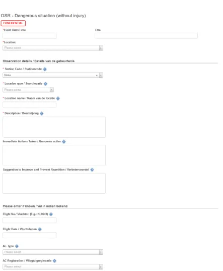
The dataset used for this research contains 19 815 samples. Each sample represents a filled report that has been categorized with one or more labels. There are 7 different types of reports that share some fields, but most of the fields are unique for each type of report. The fields contain text written using natural language in english and dutch. There are also date, numerical and categorical fields. The dataset contains 196 fields in total and it comprises reports from July 2016 to February 2019. The layout of one of such report types is shown in Figure 4.1.

There are 859 unique labels. Such labels are clustered in 13 different taxonomies as shown in Table 4.1.

Such taxonomies represent an entire hierarchy of labels, meaning that each taxonomy is a tree-like structure. The max height of a tree is 4, but most of them are 3. Here are some examples of such hierarchies:

G. External

G.3 External factors G.3.1 Drone G.3.2 Kite G.3.3 Laser

G.3.4 Volcanic ash

H. Flight

H.13 Wildlife strike

H.13.1 Birdstrike - Miscellaneous H.13.2 Multiple Birdstrike

H.13.3 Single Birdstrike H.13.4 Wildlife strike

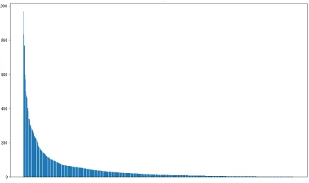
Each label has 44.99 examples on average (LAvg) with a standard deviation of 93.53.

The label density (LDen) is 0.0524. There are 72 labels with only one example. Figure 4.2

(26)

[image:26.595.65.509.129.667.2]

(27)

[image:27.595.153.472.128.364.2]

19

Table 4.1:The different taxonomies in the dataset with the number of reports that have been categorized with labels belonging to that taxonomy.

Taxonomy Frequency

A. Cargo 403

B. Consequences 3126

C. Environmental Safety - (Possible) Consequences 642 D. Environmental Safety - Causes 215 E. Environmental Safety - Event types 218 F. Environmental Safety - Processes 235

G. External 1262

H. Flight 4477

I. Ground 3671

J. Inflight 3970

K. Occupational Safety Causes 7161 L. Occupational Safety Impacts 2101

[image:27.595.175.455.400.541.2]

M. Technical 1244

Table 4.2:The different report types in the dataset with the number of reports per each type.

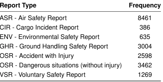
Report Type Frequency

ASR - Air Safety Report 8461 CIR - Cargo Incident Report 386 ENV - Environmental Safety Report 635 GHR - Ground Handling Safety Report 3004 OSR - Accident with Injury 2598 OSR - Dangerous situations (without injury) 3462 VSR - Voluntary Safety Report 1269

displays the histogram for the labels. It can be observed that such histogram is similar to a power-law distribution, a typical characteristic for multi-label problems.

Table 4.2 displays the different report types along with its report frequency. The air safety reports (ASR) account for almost half of the examples, followed by occupational safety reports for dangerous situation (OSR without injury).

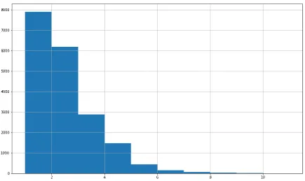
Figure 4.3 depicts the histogram of the number of taxonomies assigned to a report. It can be seen that almost eight thousand reports have been labeled with one taxonomy and around six thousand have been labeled with two taxonomies. This means that near 73% of the reports have been classified with one to two taxonomies. On average, each report has 2.02 taxonomies assigned with a standard deviation of 1.17.

(28)

[image:28.595.67.503.84.342.2]

Figure 4.2: Label distribution. The x-axis contains the labels and the y-axis depicts the report frequency. The data are ranked by report frequency.

(29)

[image:29.595.95.531.111.370.2]

21

Figure 4.3:Taxonomy count histogram. The x-axis contains the number of taxonomies as-signed and the y-axis shows the report frequency.

Table 4.3:Dataset summary. LAvgis the average number of labels per example andLDen

is the label average per number of labels. Both are calculated according to the formulas in Section 2.8.

Property Value N. samples 19 815 Date features 4 Numeric features 32 Text features 17 Categorical features 138 Other features 5 Total Fields / Features 196 N. labels 859 Taxonomies 13

LAvg 44.99±93.53

[image:29.595.220.408.536.738.2]

(30)

(31)

Chapter 5

Methodology

The main approach used in this research is to set up a quick baseline using a classical machine learning model. Setting up this quick baseline will help us to build a basic pipeline to transform the given dataset into the features that will be used to train our model. This baseline will help us to learn more about the dataset and to uncover some possible problems and mistakes in the code that trains and evaluates the different experiments.

After setting the baseline, the data were inspected to identify the features that could be cleaned and pre-processed. After identifying a possible feature, code was written to clean or pre-process such data and then its impact was assessed by running the same pipeline and comparing the metrics (macroF1and macroF0.5). This was executed in an iterative manner,

evaluating just one step at a time and incorporating the learnings gradually into our process. Beyond the well-known pre-processing steps that are commonly used by machine learning practicioners like lowercasing, stemming and removing accents, some domain specific steps were applied with the help of domain experts.

As there are several machine learning techniques that could be used to solve our prob-lem, the procedure described above was used to probe more advanced machine learning approaches and some parameters in order to identify the most promising candidates for the experiments of this research, thus reducing our search space. Figure 5.1 depicts a diagram of the described approach.

This step deemed important because the following insights were identified:

[image:31.595.87.532.639.705.2]

• The long-tail in our taxonomy distribution is problematic. The taxonomies with very

Figure 5.1:Diagram displaying the main approach used in this research. The “Change” feedback loop means that we change a pre-preprocessing step or classifier at a time according to the results of the previous iteration.

(32)

few examples represent a zero-shot learning problem that it is not important for the business objective as the company is interested in predicting frequent taxonomies correctly instead of predicting rare ones that are used for infrequent events. Therefore, labels with less than 20 examples were discarded.

• The data imbalance is problematic as well. The fact that the taxonomy distribution

resembles a power-law is giving us a taxonomy with almost 800 examples while hav-ing tens of taxonomies only with 20 examples (after the cutoff value). A quick test on our baseline helped to identify that using the synthetic minority over-sampling tech-nique(SMOTE) [30] worked way better than any other imbalanced learning techniques for multi-labeled data.

• In the text preprocessing aspect, using word unigrams delivered equal or better results

than using bigrams, or charn-grams(n= 3,4,5).

• The high dimensionality of the post-processed features affected the performance of the

classifiers. Different dimensionality reduction techniques were tested. Principal com-ponent analysis, latent semantic analysis, χ2 _{based feature selection and recursive}

feature elimination resulted in little improvement to our task.

• A very promising gradient boosting decision tree was identified: LightGBM [43]. The

preliminary results demonstrated that it was performing better than other candidates like RandomForest and classifiers based in neural networks.

(33)

Chapter 6

Experimental Setup

In this section we present the different experiments that we carry out in order to generate data that will support the answers to our request sections.

6.1 Baseline

In order to quantify the improvements achieved in this thesis, a baseline was established using two fast and popular models. Our first step is to pre-process the dataset as follows:

• The fields containing “yes/no/NA” were normalized, because some of them contained

“yes” and “no” while others had “on” and “off”. Invalid values were imputed as “NA” because some examples contained random text1_{in such fields.}

• The categorical fields were lowercased.

• English stop words were removed from text fields using the stop words list in [44].

• The text fields were tokenized using the regular expression “\b\w\w+\b”.

• The text fields were encoded using TF-IDF.

• The categorical fields were one-hot encoded.

• The numerical and date fields were excluded as they didn’t improve the baseline

per-formance.

After the pre-processing, a first model was trained using the BR method with logistic regression (LR) as base classifier. The second model is a decision tree classifier in a multi-label setting (MLDT). The implementation provided by [44] version 0.20.2 was used with the default parameters: l2 regularization, tolerance1−4 and liblinear solver for LR; gini criterion,

the minimum samples required to split an internal node is 2 and the minimum number of samples required to be a leaf node is 1 for MLDT.

1_{Some report fields containing unrelated text information were reused by the system administrator to store}

the values for some categorical fields, resulting in some samples containing invalid values for the categorical fields.

(34)

6.2 Pre-processing

For all the experiments described in the following sections we built a feature pipeline that is composed as follows:

• Remove the labels that have less than 20 examples.

• The fields containing “yes/no/NA” were normalized, because some of them contained

“yes” and “no” while others had “on” and “off”. Invalid values were imputed as “NA” because some examples contained random text2_{in such fields.}

• Some domain specific field pre-processing was applied. This included using special

tokens in the form “<token-type>” to replace unique identifiers for baggage, runways,

aircraft, written forms, unit load devices (ULD) and flights. The dates were also re-placed for a special token “<date>”.

• The categorical fields were lowercased.

• All the text fields were concatenated together.

• All the accented characters were converted to their unaccented counterparts.

• Tokenize text fields using the regular expression “(?u)<?\b\w\w+\b>?”. Such regular

expression preserved the special tokens that replaced the identifiers and dates.

• Stemming with the Lancaster algorithm [45] was applied to the text fields.

• The categorical fields were one-hot encoded.

• The numerical and date fields were excluded as they didn’t improve the baseline

per-formance.

• We only use the ten thousand most frequent text tokens.

6.3 Multi-label Classification

The machine learning techniques for our experiment were selected as follows: logistic re-gression (LR), LightGBM (LGBM) [43], multi-label decision tree (MLDT), support vector ma-chines (SVM), Classifier Chain (CC) [46], FastXML [33], PfastXML, PfastReXML [36] and DiSMEC [35]. They were selected because they presented good results in research papers when applied to problems similar to ours. They were also selected because they provided an implementation for scikit-learn [44] or their provided implementations were relatively easy to adapt to scikit-learn’s pipeline. The objective of this experiment is to identify the multi-label techniques that can be applied in the upcoming experiments. The outcome of this

2_{Some report fields containing unrelated text information were reused by the system administrator to store}

(35)

6.4. TEXTREPRESENTATION 27

experiment is to use BR and CC with LGBM, SVM, DT and LR. The other techniques were discarded.

6.4 Text Representation

For evaluating the text representation techniques, term frequency (TF), term frequency in-verse document frequency (TF-IDF), W2Vec and FastText were selected. For W2Vec we used a pre-trained model that was trained using the Google News dataset as described in [47]. For FastText a pre-trained model that was trained on the Common Crawl with sub-word information [48] was used. Both pre-trained models have a dimension of 300 and are available publicly3_{. Having such dimensions to represent a single word or token implies that}

even a short text will have a highly dimensional representation. This high dimensionality pro-duces a problem to our current compute capability. Additionally, applying this technique to texts will yield a different dimension per example and most of the machine learning models require a fixed dimension input. A possible solution is to have a fixed document length that requires longer documents to be truncated and shorter documents to be padded with zeros or any other value. This solution has the disadvantage that it still has a high dimensionality when documents tend to be long. A more plausible solution is to sum or average the resulting vectors by document. Such approach has the downside that some information is lost in the process but the dimensionality is reduced dramatically. For this same reason and because we do not have enough computational resources, state of the art techniques like ELMo and BERT were not considered. The mentioned representation techniques were evaluated using the following experiment: we train the four selected classifiers (LGBM, SVM, DT and LR) in a binary relevance setting with each of the text representation techniques, so we simulate an end-to-end evaluation and the performance of the models is compared. The classifier chain was not used because their predictions cannot be made in parallel, meaning that the evaluations would have taken too much time to complete. The outcome of this experiment is to select TF and TF-IDF as text representation techniques. They not only perform better than embeddings in this case, but have a much smaller memory footprint, because it is not needed to load the pre-trained weights.

6.5 Imbalanced Learning

After deciding the text representation, it was necessary to determine if oversampling our dataset with SMOTE can improve the performance of the classifiers. Therefore, we trained the four selected classifiers (LGBM, SVM, DT and LR) in a binary relevance setting with SMOTE and compared them against their imbalanced counterparts. This was done for both TF and TF-IDF text representation techniques. It was a big surprise to discover that the performance of LGBM improves dramatically by using SMOTE, while it affects negatively the performance of the decision trees.

(36)

6.6 Hierarchical Classification

To assess the performance of hierarchical classification over flat classification, we compare a classifier without any information about the label hierarchy against a hierarchy of classifiers based on the ideas from [40]. In this case, we leverage the fact that our labels are divided in different trees. We train a multi-label classifier to choose which trees should be applied to the report and we train a multi-label classifier per each tree that will give us the leaf labels. At prediction time, we run a taxonomy classifier on the example to get which of the thirteen taxonomies the example belongs to. Then, for each of such predicted taxonomies, we retrieve its respective trained leaf node classifier and run the example through it. The final prediction is the concatenation of the individual predictions emitted by the leaf node classifiers. The name for this classifier is local classifier per taxonomy and leaves (LCTL). Consequently, we select the best performing techniques in our previous experiments and use them as base classifiers for the LCTL approach. Then we proceed compare them against the results of such classifiers in a flat setting. The results of this experiment show that using LCTL results in a slight performance improvement against their flat counterparts.

6.7 Classifier Per Report Type

The high feature dimensionality represents a big problem for all the evaluated machine learn-ing models, even after keeplearn-ing only the top ten thousand text tokens. With the objective of further reducing such dimensionality, we assume that the data for each type of report are independent. This is further supported by the fact that each report type has a lot of unique fields. Furthermore, some fields may be shared by several reports but they contain informa-tion with totally different distribuinforma-tions because each report aims to gather different types of information. This could lead to the case where certain classifier learns some pattern for one type of report that is immediately “unlearned” due to the patterns found in another type of report. Following these assumptions, we can train one model per each report type. While such assumptions might not be completely true, training one model per report reduces the amount of features each model has to focus on and effectively increases the model perfor-mance.

To evaluate the impact of training a model per report type, we compare this approach with the results of the experiments described before. This means that we train the per report model in both flat and LCTL settings with different base classifiers.

(37)

6.8. TECHNICALEVALUATION 29

6.8 Technical Evaluation

All the experiments are performed using 5-fold cross validation with iterative stratification for multi-label data [49]. For each experiment we calculate the precision, recall, F1 and F0.5 metrics, aggregating them using microaveraging and macroaveraging as explained in

Section 2.8. The parameters used to train all the models are detailed in Appendix A.2.

6.9 Human Evaluation

The expressed concerns about the process of categorizing the reports by the human an-alysts derived in the secondary goal of this research. The development of the first goal to apply machine learning to automatically classify the safety reports confirmed such con-cerns: the trained models for taxonomies with a considerable amount of examples were not performing as expected.

In order to diagnose such problem, the misclassified examples were examined. It was discovered that labels are partially missing from some examples. To a lesser extent, it was also discovered that some labels were incorrectly assigned. Such discoveries led us to examine the current categorization process which is described in the next paragraph.

The analysts specialize in one, two or three types of reports. This means that some do-main knowledge is required to analyze each type of report. The analysts come from different backgrounds. Some of them are full-time analysts while others work part-time. In certain cases, temporary analysts will categorize some reports. A single report will be categorized by just one analyst and saved into the database. Once a report has been labeled, the label-ing outcome won’t be checked again by another analyst. This situation has a few exceptions such as an analyst reviewing a report for historical reasons and then “fixing” the labels after considering that something is not right. It is important to consider that the categorization is done among other tasks that need to be performed in the analysis of the same report, which means that the analyst’s attention and expertise is not only focused on categorizing reports. Additionally, we have identified that it is not completely clear when certain labels should be applied. During the training process that the analysts go through, they are handed some documentation about the taxonomies and how to apply certain labels, however, such docu-mentation is not extensive. Even though some label names are self-descriptive, this could be not enough and a clear description should be provided. Furthermore, the big taxonomy poses a problem because it is not feasible for the analyst to go through the entire list of possible labels to annotate the report with the exact labels as pointed out by [36]. Given this fact, we cannot consider our current dataset as the golden ground truth for our machine learning effort, meaning that there exists the possibility that a prediction is marked as a false positive while it is a true positive.

We strongly believe that some of the theories of content analysis [25] can be used to measure and improve the report categorization process. Consequently, we arrange an ex-periment to measure the reliability of the process using Krippendorff’s multi-valued α for

(38)

point to solve the problems exposed above.

The experiment was carried out with 5 analysts that participated voluntarily. Each analyst was asked to review up to 50 real reports according to the report types that they categorize in their day to day work. If an analyst normally categorizes more than one report type, the 50 reports will contain a proportional amount of each report type. This proportion is calcu-lated over the report type distribution in our dataset, which means, that stratified sampling was employed instead of sampling them uniformly. To make things clear, if two analysts specialize on the ASR type, each analyst will label the same 50 ASR reports. For the case of those categorizing GHR, CIR and ENV types; each analyst will need to classify the same 37 GHR, 5 CIR, and 8 ENV reports. The number of 50 reports was agreed with the analysts according to their workload.

A web application was created in order to gather the data for this experiment. The user interface was designed to be the most similar to the application they normally use to categorize the reports. An screenshot of such user interface is displayed in Appendix A.3. It was decided to create such application because we wanted the analysts to use a single interface to read and categorize the reports. Additionally, as the reports for this experiment were real, the web application allowed us to hide the labels for the reports that were already classified, therefore preventing bias. The results were collected anonymously, so we cannot trace back the answers to a particular analyst.

(39)

Chapter 7

Results & Discussion

The results of all the experiments that were executed during this project are presented in the following subsections.

The following abbreviations are used in the tables: binary relevance (BR), logistic regres-sion (LR), LightGBM (LGBM), deciregres-sion tree (DT), multi-label deciregres-sion tree (MLDT), support vector machines (SVM) and Classifier Chain (CC). Binary relevance and classifier chain are methods that require a base classifier, therefore, we announce the respective method fol-lowed by the base classifier used. For example, BR LR means that the method used is binary relevance with a logistic regression base classifier.

Even though we report diverse metrics for our experiments, we are looking to optimize the macro F0.5 measure. We chose the macro average because we have an unbalanced

dataset with almost a power-law distribution. Macroaveraging gives equal importance to each class, making it suitable to evaluate the overall model in our case. TheF0.5 metric was

chosen by business needs (see Section 2.8).

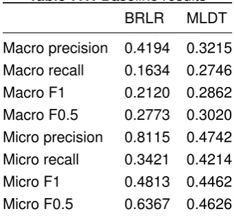
7.1 Baseline Evaluation

[image:39.595.227.398.594.753.2]

Table 7.1 displays the results obtained using a 5-fold cross validation.

Table 7.1:Baseline results BRLR MLDT Macro precision 0.4194 0.3215 Macro recall 0.1634 0.2746 Macro F1 0.2120 0.2862 Macro F0.5 0.2773 0.3020 Micro precision 0.8115 0.4742 Micro recall 0.3421 0.4214 Micro F1 0.4813 0.4462 Micro F0.5 0.6367 0.4626

(40)

7.2 Machine Learning Models Evaluation

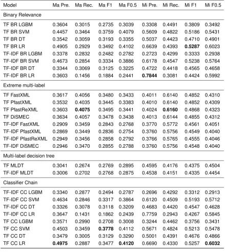
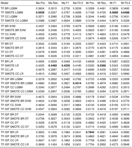
In this section we present the results of using different machine learning models to solve this specific problem. Such results are displayed in table 7.2. The evaluated models are compared using both term frequency (TF) and term frequency inverse document frequency (TF-IDF). The multi-label model classifier chain using logistic regression or SVM as base classifier performed best, followed by binary relevance with logistic regression or SVM as base classifiers as well. These four best models have in common that they all use term frequency as text representation features. The extreme multi-label techniques with TF have the best recall and an acceptable performance in the rest of the metrics. These results suggest that our problem of report classification still lies in the area of classic multi-label classification. Even though the number of labelsLis greater than eight hundred, it is feasible

to train BR in less than an hour using multiple cores in a regular laptop computer, and thus extreme multi-label classification is not needed.

Unfortunately, CC is a method that is slower than BR. Although its complexity is almost the same as BR if L is small [46], this is not the case. Additionally, the predictions for classifier chain models cannot be parallelized, imposing a big performance penalty. Therefore, it is not possible to always evaluate it in further experiments.

7.3 Text Representation Evaluation

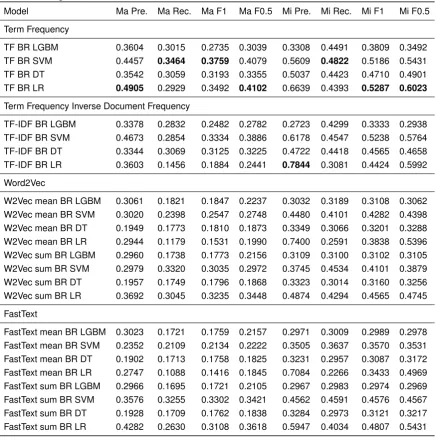
In this section we present the impact of using recent word embeddings over TF-IDF for this particular problem that involves multi-label learning and hierarchical classes. Word2Vec (W2Vec) and FastText embeddings are aggregated using sum and average (mean) methods. The experiment results are listed in Table 7.3.

It is clear that TF and TF-IDF outperform the other methods. For the embeddings case, summing always performs better than averaging. FastText sum ranks 4th place, meaning that is the best performer for the embeddings. It is important to note that the fact that we are averaging or summing such embeddings can seriously affect their performance because we inevitably lose some information in the aggregation process. However, not aggregating them derives in a even higher feature dimensionality, becoming prohibitive for our research.

7.4 Imbalanced Learning Evaluation

(41)

[image:41.595.92.532.203.695.2]

7.4. IMBALANCEDLEARNINGEVALUATION 33

Table 7.2:Machine Learning models experiment results. The results are macro and micro averaged.

Model Ma Pre. Ma Rec. Ma F1 Ma F0.5 Mi Pre. Mi Rec. Mi F1 Mi F0.5 Binary Relevance

TF BR LGBM 0.3604 0.3015 0.2735 0.3039 0.3308 0.4491 0.3809 0.3492 TF BR SVM 0.4457 0.3464 0.3759 0.4079 0.5609 0.4822 0.5186 0.5431 TF BR DT 0.3542 0.3059 0.3193 0.3355 0.5037 0.4423 0.4710 0.4901 TF BR LR 0.4905 0.2929 0.3492 0.4102 0.6639 0.4393 0.5287 0.6023 TF-IDF BR LGBM 0.3378 0.2832 0.2482 0.2782 0.2723 0.4299 0.3333 0.2938 TF-IDF BR SVM 0.4673 0.2854 0.3334 0.3886 0.6178 0.4547 0.5238 0.5764 TF-IDF BR DT 0.3344 0.3069 0.3125 0.3225 0.4722 0.4418 0.4565 0.4658 TF-IDF BR LR 0.3603 0.1456 0.1884 0.2441 0.7844 0.3081 0.4424 0.5992 Extreme multi-label

TF FastXML 0.3617 0.4056 0.3480 0.3433 0.4011 0.6140 0.4852 0.4310 TF PfastXML 0.3532 0.4035 0.3445 0.3383 0.4010 0.6140 0.4852 0.4309 TF PfastReXML 0.3603 0.4075 0.3495 0.3441 0.4024 0.6160 0.4868 0.4323 TF DiSMEC 0.3634 0.4057 0.3478 0.3438 0.4013 0.6144 0.4855 0.4312 TF-IDF FastXML 0.2909 0.3459 0.2843 0.2768 0.3770 0.5772 0.4561 0.4051 TF-IDF PfastXML 0.2869 0.3449 0.2836 0.2754 0.3760 0.5756 0.4549 0.4040 TF-IDF PfastReXML 0.2949 0.3456 0.2858 0.2792 0.3766 0.5765 0.4555 0.4046 TF-IDF DiSMEC 0.2946 0.3470 0.2855 0.2788 0.3760 0.5756 0.4548 0.4040 Multi-label decision tree

TF MLDT 0.3041 0.2674 0.2769 0.2895 0.4595 0.4176 0.4375 0.4504 TF-IDF MLDT 0.3006 0.2702 0.2768 0.2875 0.4538 0.4151 0.4335 0.4454 Classifier Chain

(42)

[image:42.595.66.503.226.667.2]

Table 7.3: Text representation experiment results. The results are macro and micro aver-aged.

Model Ma Pre. Ma Rec. Ma F1 Ma F0.5 Mi Pre. Mi Rec. Mi F1 Mi F0.5 Term Frequency

TF BR LGBM 0.3604 0.3015 0.2735 0.3039 0.3308 0.4491 0.3809 0.3492 TF BR SVM 0.4457 0.3464 0.3759 0.4079 0.5609 0.4822 0.5186 0.5431

TF BR DT 0.3542 0.3059 0.3193 0.3355 0.5037 0.4423 0.4710 0.4901

TF BR LR 0.4905 0.2929 0.3492 0.4102 0.6639 0.4393 0.5287 0.6023

Term Frequency Inverse Document Frequency

TF-IDF BR LGBM 0.3378 0.2832 0.2482 0.2782 0.2723 0.4299 0.3333 0.2938 TF-IDF BR SVM 0.4673 0.2854 0.3334 0.3886 0.6178 0.4547 0.5238 0.5764 TF-IDF BR DT 0.3344 0.3069 0.3125 0.3225 0.4722 0.4418 0.4565 0.4658 TF-IDF BR LR 0.3603 0.1456 0.1884 0.2441 0.7844 0.3081 0.4424 0.5992 Word2Vec

W2Vec mean BR LGBM 0.3061 0.1821 0.1847 0.2237 0.3032 0.3189 0.3108 0.3062 W2Vec mean BR SVM 0.3020 0.2398 0.2547 0.2748 0.4480 0.4101 0.4282 0.4398 W2Vec mean BR DT 0.1949 0.1773 0.1810 0.1873 0.3349 0.3066 0.3201 0.3288 W2Vec mean BR LR 0.2944 0.1179 0.1531 0.1990 0.7400 0.2591 0.3838 0.5396 W2Vec sum BR LGBM 0.2960 0.1738 0.1773 0.2156 0.3109 0.3100 0.3102 0.3105 W2Vec sum BR SVM 0.2979 0.3320 0.3035 0.2972 0.3745 0.4534 0.4101 0.3879 W2Vec sum BR DT 0.1957 0.1749 0.1796 0.1868 0.3323 0.3014 0.3160 0.3256 W2Vec sum BR LR 0.3692 0.3045 0.3235 0.3448 0.4874 0.4294 0.4565 0.4745 FastText

(43)

7.5. HIERARCHICALCLASSIFICATIONEVALUATION 35

used in conjunction with LGBM and LR, both in a BR setting. On the other hand, DT has had a consistent poor performance so far, therefore we decide to discard it.

7.5 Hierarchical Classification Evaluation

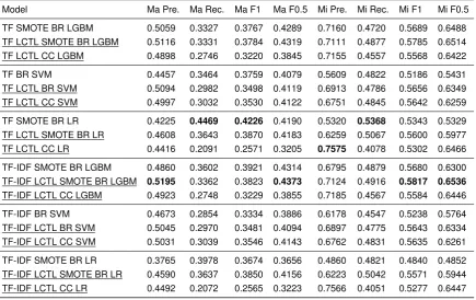
The results of the experiment to assess the impact of hierarchical classification over flat clas-sification are displayed in Table 7.5. We evaluate LGBM, SVM and LR with TF and TF-IDF in a local classifier per taxonomy and leaves (LCTL) mode. Then, we proceed to compare them to their flat counterparts. We run each possible combination in binary relevance and classifier chain multi-label settings. LGBM and LR in a binary relevance setting are evalu-ated using SMOTE oversampling because those are the only models that benefit from that technique. It can be seen that LCTL brings a slight improvement in the performance of most of the classifiers.

7.6 Classifier Per Type of Report Results

To test our hypothesis that training one independent classifier per report type performs better than training one classifier for the entire dataset, we used this proposed technique with the best combinations that resulted from previous experiments. The results are presented on Table 7.6.From the table is clear that the combination of TF-IDF, SMOTE, BR and LGBM per report type outperforms any other model that has been evaluated in this research. It can also be concluded that training one classifier per each report type brings moderate to big performance improvements for the evaluated models. On the other hand, using LCTL does not perform that well. We hypothesize that training per report type divides the search space well enough, meaning that the additional partitioning brought by LCTL is of little help.

7.7 Inter-annotator Agreement

The inter-annotator agreement measure mvα is 57.45%. The 5 analysts labeled in total

160 out of 250 reports. Unfortunately, the holiday season coincided with our experiment, preventing the analysts to label the entire selected sample for this experiment. Between the 160 labeled reports, 34 were comparable, meaning that at least two analysts labeled the same 34 reports, which is a requirement for the metric. The agreement results were calculated using the open source software1_{provided by the}

mvα authors [28].

The result of mvα = 57.45% is difficult to interpret. [25] recommends that conclusions

should not be made about data with less than 66.7%. However, the authors “recommend such levels with considerable hesitation. The choice of reliability standards should always be related to the validity requirements imposed on the research results, specifically to the costs of drawing wrong conclusions”. The authors also mention guidelines that have been

(44)

[image:44.595.67.503.203.690.2]

Table 7.4: Results of performing SMOTE oversampling. The results are macro and micro averaged.

Model Ma Pre. Ma Rec. Ma F1 Ma F0.5 Mi Pre. Mi Rec. Mi F1 Mi F0.5 TF BR LGBM 0.3604 0.3015 0.2735 0.3039 0.3308 0.4491 0.3809 0.3492 TF SMOTE LGBM 0.5059 0.3327 0.3767 0.4289 0.7160 0.4720 0.5689 0.6488 TF CC LGBM 0.3571 0.2990 0.2708 0.3008 0.3244 0.4462 0.3756 0.3431 TF SMOTE CC LGBM 0.3388 0.2967 0.2624 0.2889 0.3134 0.4444 0.3674 0.3329 TF BR SVM 0.4457 0.3464 0.3759 0.4079 0.5609 0.4822 0.5186 0.5431 TF SMOTE BR SVM 0.4439 0.3436 0.3731 0.4053 0.5603 0.4817 0.5180 0.5426 TF CC SVM 0.4503 0.3459 0.3778 0.4112 0.5671 0.4824 0.5213 0.5478 TF SMOTE CC SVM 0.4509 0.3473 0.3789 0.4121 0.5674 0.4809 0.5206 0.5477

TF BR DT 0.3542 0.3059 0.3193 0.3355 0.5037 0.4423 0.4710 0.4901

TF SMOTE BR DT 0.2815 0.3434 0.3011 0.2875 0.3770 0.4679 0.4175 0.3922

TF CC DT 0.3479 0.3005 0.3129 0.3290 0.5001 0.4391 0.4676 0.4866

TF SMOTE CC DT 0.3494 0.3026 0.3153 0.3311 0.4981 0.4367 0.4653 0.4844

TF BR LR 0.4905 0.2929 0.3492 0.4102 0.6639 0.4393 0.5287 0.6023

TF SMOTE LR 0.4225 0.4469 0.4226 0.4190 0.5320 0.5368 0.5343 0.5329

TF CC LR 0.4975 0.2887 0.3477 0.4120 0.6690 0.4330 0.5257 0.6032

(45)

[image:45.595.96.532.181.455.2]

7.7. INTER-ANNOTATORAGREEMENT 37

Table 7.5:Hierarchical classification experiment results. Hierarchical models are under-lined. The results are macro and micro averaged.

Model Ma Pre. Ma Rec. Ma F1 Ma F0.5 Mi Pre. Mi Rec. Mi F1 Mi F0.5

TF SMOTE BR LGBM 0.5059 0.3327 0.3767 0.4289 0.7160 0.4720 0.5689 0.6488

TF LCTL SMOTE BR LGBM 0.5116 0.3331 0.3784 0.4319 0.7111 0.4877 0.5785 0.6514

TF LCTL CC LGBM 0.4898 0.2746 0.3220 0.3845 0.7155 0.4557 0.5568 0.6422

TF BR SVM 0.4457 0.3464 0.3759 0.4079 0.5609 0.4822 0.5186 0.5431

TF LCTL BR SVM 0.5094 0.2982 0.3498 0.4119 0.6913 0.4786 0.5656 0.6349

TF LCTL CC SVM 0.4997 0.3032 0.3530 0.4122 0.6751 0.4845 0.5642 0.6259

TF SMOTE BR LR 0.4225 0.4469 0.4226 0.4190 0.5320 0.5368 0.5343 0.5329

TF LCTL SMOTE BR LR 0.4608 0.3643 0.3870 0.4183 0.6259 0.5067 0.5600 0.5977

TF LCTL CC LR 0.4416 0.2091 0.2571 0.3205 0.7575 0.4078 0.5302 0.6466

TF-IDF SMOTE BR LGBM 0.4860 0.3602 0.3921 0.4314 0.6795 0.4879 0.5680 0.6300

TF-IDF LCTL SMOTE BR LGBM 0.5195 0.3362 0.3823 0.4373 0.7124 0.4916 0.5817 0.6536

TF-IDF LCTL CC LGBM 0.4923 0.2748 0.3229 0.3855 0.7185 0.4567 0.5584 0.6446

TF-IDF BR SVM 0.4673 0.2854 0.3334 0.3886 0.6178 0.4547 0.5238 0.5764

TF-IDF LCTL BR SVM 0.5045 0.2970 0.3481 0.4094 0.6897 0.4775 0.5643 0.6334

TF-IDF LCTL CC SVM 0.5031 0.3039 0.3546 0.4143 0.6762 0.4831 0.5635 0.6261

TF-IDF SMOTE BR LR 0.3765 0.3978 0.3674 0.3656 0.4860 0.4821 0.4840 0.4852

TF-IDF LCTL SMOTE BR LR 0.4590 0.3637 0.3850 0.4156 0.6223 0.5042 0.5571 0.5944

TF-IDF LCTL CC LR 0.4492 0.2072 0.2565 0.3223 0.7566 0.4051 0.5277 0.6447

Table 7.6:Results of training one classifier per report type. The results are macro and micro averaged.

Model Ma Pre. Ma Rec. Ma F1 Ma F0.5 Mi Pre. Mi Rec. Mi F1 Mi F0.5

TF-IDF SMOTE BR LGBM 0.5717 0.4136 0.4541 0.5022 0.7400 0.5450 0.6277 0.6906

TF-IDF LCTL SMOTE BR LGBM 0.5674 0.4189 0.4558 0.5015 0.7139 0.5420 0.6162 0.6713

TF SMOTE BR LR 0.4987 0.4782 0.4770 0.4860 0.6131 0.5870 0.5997 0.6076

TF LCTL SMOTE BR LR 0.5011 0.4718 0.4740 0.4854 0.6095 0.5699 0.5891 0.6012

TF-IDF CC SVM 0.4973 0.3336 0.3797 0.4304 0.6464 0.5023 0.5653 0.6113

[image:45.595.93.533.612.710.2]

(46)

proposed for Cohen’sκ, which can be applicable to Krippendorff’s α. For this reason, we

believe that we can use the interpretations for Cohen’s κ proposed by [26] to interpret the

mvαcalculated in this research. The paper proposes that a value between 40% and 59% is

considered a weak agreement.

7.8 Comparison to Related Work

Researchers in [31] apply Natural Language Processing (NLP) techniques to create an avi-ation safety report threshold-based classifier using correlavi-ations between the labels and the extracted linguistic features. These correlations are weighted by document length and the final classification is decided by a set of thresholds and manual rules. In contrast, our re-search performs the classification based on learning the rules automatically from data, with-out any manual rules. Unfortunately, the authors do not provide any metrics to compare our approaches.

[32] apply NLP and binary relevance with support vector machines (BR SVM) to classify aviation safety reports automatically. They report a microaverageF1of 79.15% in their best

model. Our best model reports aF1of 62.77%. Our problem is considered harder because

(47)

Chapter 8

Conclusion

8.1 Conclusion

Based on the experimental results, it can be concluded that classical multi-label machine learning techniques can be applied successfully to the problem of automatic safety reports classification.

The answer to RQ1is stated as follows: the accuracy of applying machine learning to classify aviation safety reports automatically is influenced mainly by training one classifier per each type of report and the use of classical multi-label categorization techniques.

The baseline that was established with logistic regression is improved by 81% employing our proposed configuration that trains a LGBM classifier in a binary relevance setting per each type of report while using a TF-IDF text representation with SMOTE oversampling. This configuration achieves a macroaveraged F0.5 score of 50.22%. Our results suggest

that using aggregated embeddings does not bring any benefits to our classification task. TF and TF-IDF clearly outperform the embeddings when tested in downstream tasks for the report classification. Additionally, TF and TF-IDF are less computationally expensive to train and to evaluate the models.

Using a simple multi-label learning model like binary relevance has the best impact in the performance of the classification task. In our specific case, the performance gain surpasses the fact that it is computationally more expensive when compared to extreme multi-label models. Additionally, it is still feasible to train binary relevance models in commodity hard-ware given our current dataset.

The use of SMOTE oversampling improves the performance of LGBM when used in combination with binary relevance by 41%. The performance of logistic regression is also improved to a lesser extent. SVM and classifier chain (CC) do not perceive any benefit by the use of SMOTE.

Using hierarchical classification with LCTL slightly improves the performance of most classifiers. However, our results suggest that the performance is decreased when a LCTL classifier is trained per each report type.

Training one classifier per report type offers a substantial improvement in classification performance. We believe that this method decreases the feature dimensionality and sparsity

(48)

dramatically. Additionally we assume that the data for each type of report are independent. Such assumptions proved to be valid as the classification performance was improved by the application of this strategy.

With respect to theRQ2, the report classification process reliability should be measured using Krippendorff’s mvα. Our reliability study showed a mvα of 57.45%, which can be

interpreted as a weak agreement. Therefore, the labeling process needs to be improved. We recommend to the organization to aim to improve the metric to a 66.7% which is considered a moderate agreement.

8.2 Limitations

There are important limitations to this research. In the text representation evaluation, we aggregate Word2Vec and FastText embeddings using sum or average (see Section 6.4), possibly affecting their representational capacity. This decision was made in order to keep the computation feasible with our current infrastructure. We do not claim that this is the best approach. There are other ways to limit the high dimensionality that such techniques bring, like truncating the text up to a certain length. Furthermore, we were not able to evaluate state of the art techniques like ELMo and BERT due to their high demand of GPU resources.

In the same way, the fact that we merge all the report text fields is seen as a limitation. This decision was made again to keep the experiment within the boundaries of our current infrastructure.

In the hierarchical classification experiment we exclusively evaluate LCTL, which uses only two levels of the hierarchy. Although the results are promising, it is needed to further evaluate the impact of exploiting the full hierarchy and the use of more advanced approaches for hierarchical classification.

We assume the report types to be independent, which represents a limitation because some reports share fields. Therefore, discovering the correlations between the report types and their fields could bring better insights about how to further improve the classification performance.

An additional limitation of this research is that we do not use propensity scored metrics. We argue in Section 6.9 that we do not consider our dataset as the “gold” ground truth because every example may have missing labels. Therefore, we can erroneously treat a correct prediction as a false positive. Using propensity scored metrics addresses this limita-tion, as they provide unbiased estimates of the metric computed on the “gold” ground truth. See [36] for a further explanation about this rationale.