Overhauser dynamic nuclear polarisation studies in solution state at 3 4T

(1)

University of Warwick institutional repository: http://go.warwick.ac.uk/wrap

A Thesis Submitted for the Degree of PhD at the University of Warwick

http://go.warwick.ac.uk/wrap/57817

This thesis is made available online and is protected by original copyright.

Please scroll down to view the document itself.

(2)

Overhauser Dynamic Nuclear Polarisation Studies

in Solution-State at 3.4T

by

Thomas Kai Yip Tam

Thesis

Submitted to the University of Warwick

for the degree of

Doctor of Philosophy

Department of Physics

(3)

List of Tables

5.1 Summary of DNP enhancements and coupling factor data for several studies conducted at 3.4 T . . . 76

6.1 Summary of relaxation time and enhancement measurements used to estimate leakage factors and coupling factors in three different

samples of organic compounds in aqueous solutions. . . 110

7.1 Summary of dual irradiation DNP experiment results for 5 mM 4-oxo-TEMPO-d16-15N in toluene, showing the effect of increasing

satura-tion of second EPR transisatura-tion onε. Experiments where all microwave

power is applied on-resonance have been emphasised in the table with bold font and double arrows; ‘L’ and ‘S’ indicate ‘large’ and ‘small’

changes in enhancement, respectively (arbitrarily defined as >15%

and <15%). . . 120 7.2 Summary of dual irradiation DNP experiment results for 2.5 mM

TEMPOL in toluene, showing the effect of increasing saturation of a

second EPR transition onε. Experiments with Source B and A irradi-ating allowed EPR transitions are highlighted with enhancements in

bold and enhancement change represented by double arrows; ‘L’ and

(7)

List of Figures

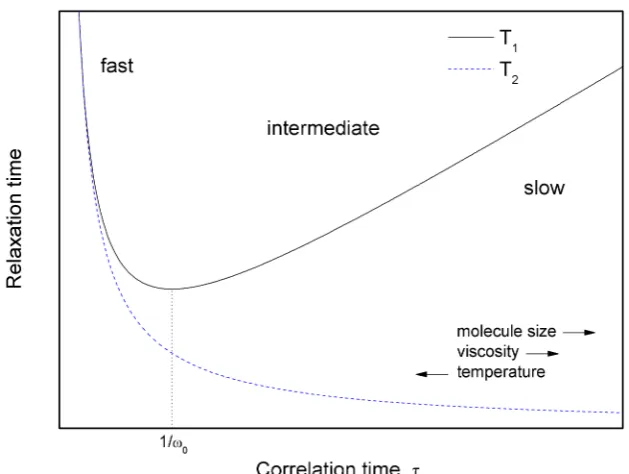
2.1 Lorentzian spectral density functions showing molecular motion in the slow, intermediate and fast regimes. . . 10

2.2 Plot illustrating the variation of the spin-lattice (1/T1 ∝ τc/(1 +

(ω0τc)2)) and spin-spin (1/T2∝3J(0) + 5J(ω0) + 2J(2ω0)) relaxation

time constants with the correlation time of molecular motion [16].

Regions for slow, intermediate and fast motion are indicated, as well as the effect of increasing molecule size, liquid viscosity and

temper-ature on relaxation. . . 10

2.3 Energy levels resulting from the Zeeman effect and hyperfine splitting for an S = 1/2 electron and I = 1 nucleus. The 3 allowed EPR

transitions are indicated by the blue arrows, corresponding to an

energy gaphν. . . 17 2.4 Energy level diagram for an electron spin S = 1/2 coupled to a

nu-clear spin I = 1/2. All possible transition probabilities are shown,

where wI is the nuclear spin relaxation rate, wS is the electron spin

relaxation rate, w2 is the double-quantum relaxation rate, w0 is the

zero-quantum relaxation rate. The microwave excitation of an

elec-tron transition is also indicated. . . 20 2.5 Calculated field dependence of coupling factor for pure dipolar

re-laxation, modeled with rotational (solid black line) and translational

(dashed blue line) diffusion, using a correlation time τ = 20 ps. . . . 25

3.1 Theoretical field dependence of coupling factors, calculated using a

20 ps correlation time (from Reference [33]). Top 2 lines — pure

dipo-lar relaxation mechanism, modelled with rotational and translational diffusion; bottom 4 lines — pure scalar relaxation mechanism, shown

for various values of the fast electron spin relaxation correction termβ. 30

(8)

4.2 Photograph of the Warwick 94 GHz DNP-NMR spectrometer. . . 46

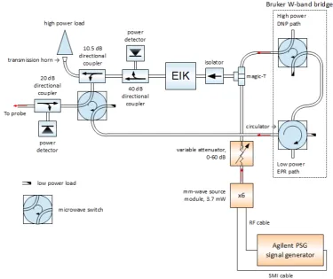
4.3 Schematic of W-band microwave bridge for Bruker ELEXSYS E680 EPR system. . . 47

4.4 EIK amplifier characteristics. . . 49

4.5 Diagram of modified ENDOR probe: (1) W-band cavity, (2) RF coil, (3a,b) RF leads, (4) sample access, (5) variable tuner, (6) coupling

iris, (7) waveguide to microwave assembly, (8) thermocouple [43]. . . 50

4.6 Structures of derivatives of the nitroxide free radical TEMPO. . . 51 4.7 Typical sample. Surface of outer capillary tube marked with red

dots with a separation of 1 mm in order to ensure proper sample

positioning in the sample holder and cavity. . . 52 4.8 One-pulse sequence. . . 53

4.9 Pulse sequences used to measure spin-lattice relaxation time T1. . . 53

4.10 Example of 94 GHz CW-EPR spectrum for 100 mM TEMPOL radical in water at room temperature. . . 55

4.11 Typical pulse sequence for Overhauser DNP experiments. . . 56

4.12 Schematic of the microwave assembly utilising two microwave sources. The orange coloured components were added as the second microwave

source, whilst the blue coloured components constitute the original setup for the experiments in Chapters 5 and 6. . . 57

4.13 Output of low-power side of Bruker W-band bridge in CW-mode,

measured using Hewlett Packard power meter. . . 59 4.14 Output of high-power side of Bruker W-band bridge in pulse-mode,

measured using Hewlett Packard power meter at the bridge and at the

magic-T output. The loss in microwave power in travelling from the bridge through to the magic-T output is plotted in red (diamonds)

and corresponds to the right-hand axis. . . 59

4.15 Output of magic-T when used with two sources simultaneously. The contributions to the total input power from each source is

approxi-mately equal. . . 60

4.16 Agilent frequency ‘sweep’ in which DNP enhancement is plotted as a function of frequency; used to determine the required input frequency

for two-source DNP experiments. DNP experiments were conducted

(9)

5.1 1H NMR spectra of water with 120 mM TEMPOL; top — no mi-crowave irradiation, 100 acquisitions; bottom — 1.3 W mimi-crowave irradiation for one second, single acquisition. . . 64

5.2 Water proton spin-lattice relaxation rates. . . 67

5.3 Proton chemical shift and inferred temperature in water as a function of duration of 1.3 W microwave irradiation, for different

concentra-tions. Dotted line — fit of the form (1−exp(−t/τT)) withτT = 0.25 s.

The inset shows the same data for 80 mM and 120 mM over an ex-tended irradiation period. . . 68

5.4 Enhancement as a function of 1.3 W microwave irradiation time for

different radical concentrations. Dotted lines are single exponent fits of the data with time constants τ displayed. The inset shows the

first second of irradiation for concentrations of 120 mM, 80 mM and

40 mM. The dotted line is once again a single exponent fit. . . 69 5.5 Evolution of nuclear spin polarisation with 1.3 W microwave

irradia-tion. Enhancement values are corrected for the change in Boltzmann

factor with temperature increase. . . 71 5.6 CW-EPR spectra of TEMPOL in water recorded at different

temper-atures, at two radical concentrations. . . 72 5.7 DNP enhancement as a function of magnetic field for a sample of

water with 120 mM TEMPOL, 10 mm length. 1 s microwave

irradi-ation. Circles — 1.3 W, 130◦C; squares — 0.25 W, 40◦C. Lines are integrated CW-EPR spectra: solid line — 98◦C; dashed line — 22◦C. 72

5.8 Simulations fitted to experimental data of DNP enhancement in water

with 100 mM TEMPOL resulting from 1.3 W microwave irradiation. 75

6.1 Skeletal formula of glycine (NH2CH2COOH). . . 82

6.2 1H NMR spectrum of 3 M glycine-100 mM TEMPOL-D2O sample:

no microwave irradiation, 40,000 acquisitions, 7.0±0.5◦C. . . 83 6.3 DNP-enhanced1H NMR spectrum of 3 M glycine-100 mM

TEMPOL-D2O. ∼1.1 W applied microwave power, 400 acquisitions, 101±3◦C. 84

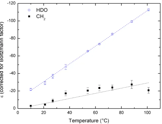
6.4 Overlay of DNP-enhanced spectra, illustrating the increasing enhance-ment and temperature of both HDO and CH2 protons. The DNP

spectra have been normalised to the same number of acquisitions

(10)

6.5 DNP enhancement as a function of temperature, as calculated from

the chemical shift. Dashed lines — linear fits with slopes of −1.01 and −0.30 for HDO and CH2 protons, respectively. Ratio of slopes

mHDO/mCH2 = 3.4±0.5. . . 86 6.6 Saturation-recovery experiment at 143 MHz. Sample temperature is

100±3◦C. Dashed lines — fit of the form (1−exp(−t/T1I)) with

resulting nuclear relaxation times displayed in the figure. . . 88

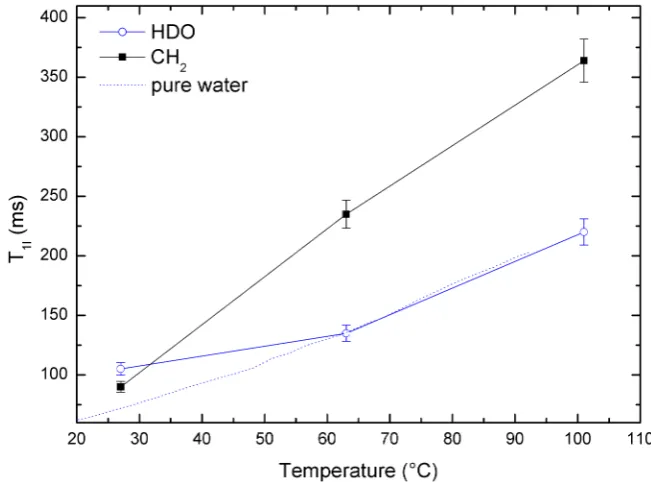
6.7 Temperature dependence of proton T1 of HDO and CH2 in water

with 3 M glycine and 100 mM TEMPOL at 143 MHz. Data are

shown with temperature indicated by chemical shift. TheT1 of pure

water is shown as a dotted line and has been scaled to agree with the glycine-TEMPOL-D2O sample value at 63◦C. . . 88

6.8 Room temperatureT1Ivalues of 3 M glycine-D2O at 143 MHz,

inter-polated from measurements made at 100 MHz and 300 MHz. . . 90 6.9 Skeletal formula of L-proline (C5H9NO2). . . 92

6.10 1H NMR spectrum of 1 M L-proline-100 mM TEMPOL-D2O sample:

no microwave irradiation, 48,000 acquisitions, 6.0±0.5◦C. . . 93 6.11 DNP-enhanced1H NMR spectrum of 1 M L-proline-100 mM

TEMPOL-D2O. ∼0.4 W applied microwave power, 200 acquisitions, 70±3◦C. 94

6.12 Overlay of DNP-enhanced spectra, demonstrating the increase of

en-hancement and temperature of HDO, C-CH2-N and C-CH2-C

pro-tons. The DNP spectra have been normalised to the same number of acquisitions and the thermal equilibrium spectrum (multiplied by a

factor of 5) is displayed on top for comparison. . . 95

6.13 DNP enhancement as a function of temperature, as calculated by chemical shift change. Dashed lines — linear fits with slopes of−1.31,

−0.48, −0.08 and −0.26 for HDO, C-CH2-N, C-CH2-C and Peak Y

protons, respectively. Ratio of slopes mHDO/mC-CH2-N = 2.8±0.4, mHDO/mC-CH2-C = 15.8±0.7,mHDO/mY= 5.1±0.6. . . 96 6.14 Effect of temperature on proton T1I of HDO and C-CH2-C in water

doped with 100 Mm TEMPOL and 1 M L-proline. Data are shown with the temperature calculated from chemical shift, and have an

uncertainty of approximately ±3◦C. The T1I of pure water has been

included, and scaled to agree with the sample value at 11◦C, for comparison. . . 97

(11)

6.16 1H NMR spectrum of acrylic acid-D2O(10:90 % v/v)-100 mM

TEM-POL sample: no microwave irradiation, 100,000 acquisitions, 6.0±

0.5◦C. . . 100

6.17 The reduction of TEMPOL by acrylic acid, resulting in the formation

of the diamagnetic TEMPOL-H molecule. . . 101 6.18 DNP-enhanced1H NMR spectrum of acrylic acid-D2O-100 mM

TEM-POL.∼1.7 W applied microwave power, 400 acquisitions, 83±3◦C. 101 6.19 Overlay of DNP-enhanced spectra, showing the increasing

enhance-ment of HDO and AA protons, whilst showing the changing shift

of HDO and constant position of AA. The DNP spectra have been

normalised to the same number of acquisitions and the thermal equi-librium signal (top) increased by a factor of 5 for comparison. . . 102

6.20 Change in nuclear spin-lattice relaxation time as a function of time,

due to reduction of TEMPOL. Measured at room temperature at 284 MHz. . . 103

6.21 Evolution of integrated X-band EPR signal intensity with time,

show-ing a continuous degradation of TEMPOL radical at room tempera-ture. Inset — expansion of the first 275 minutes after the sample was

prepared. . . 104 6.22 Temperature dependence of DNP enhancement, with temperatures

calculated from change in chemical shift of water protons. Dashed

lines — linear fits with slopes of -0.72, -0.34 and -0.14 for HDO, AA and CH3 protons, respectively. Ratio of slopes mHDO/mAA =

2.1±0.2, mHDO/mCH3 = 5.3±5.3. . . 105 6.23 Temperature dependence of proton T1I of HDO and AA protons in

D2O with acrylic acid and an initial radical concentration of 100 mM

TEM-POL which is thought to have reduced by at least ∼40%. Data are shown with temperatures indicated by HDO chemical shift. The T1I

of pure water is shown as a dotted line and has been scaled to agree

with the sample value at 4◦C. . . 107

6.24 T1I values of acrylic acid-D2O (10:90 % v/v) at 143 MHz at room

temperature, interpolated from measurements made at 100 MHz and

300 MHz. . . 108

(12)

7.2 Source A frequency sweep of 5mM 4-oxo-TEMPO-d16-15N in toluene,

used to find electron resonance frequencies at fixed magnetic field. PA≈429µW, Source B off. Arrows — frequencies used in later

ex-periments corresponding to irradiating: off-resonance (1, 5); allowed

EPR transitions (2, 4); and forbidden transitions (3). νi = 94.070,

94.155, 94.183, 94.211, 94.300 GHz; fori= 1, 2,... 5. . . 117

7.3 Dual irradiation experiment with Source B irradiating on-resonance

at ν4 with constant power (PB ≈ 78 µW), whilst simultaneously

ramping Source A power (PA≈10–429µW) off-resonance atν1.

In-set — measured diode voltages indicating transmitted and reflected

power. . . 118 7.4 Irradiation of both hyperfine lines. Source B at ν4 with constant

power (PB ≈ 78 µW), ramping Source A power (PA ≈ 10–429 µW)

atν2. . . 118

7.5 Source A frequency sweep of 2.5 mM TEMPOL in toluene, used to

find electron resonance frequencies at fixed magnetic field. PA ≈

PB ≈78 µW. Arrows — frequencies used in later experiments

corre-sponding to irradiating: off-resonance (1, 7); the allowed EPR

tran-sitions (2, 4, 6); and forbidden trantran-sitions (3, 5). νi = 94.100, 94.163,

94.185, 94.205, 94.230, 94.246, 94.300 GHz; fori= 1, 2,... 7. . . 121

7.6 Dual irradiation experiment with Source B irradiating central

transi-tion (ν4) with constant power (PB ≈78 µW), whilst simultaneously

ramping Source A power (PA≈ 10–429µW) off-resonance atν1. . . 122

7.7 Irradiation of two hyperfine lines. Source B at central transition (ν4)

with constant power (PB≈78µW), ramping Source A power (PA≈

10–429µW) at low frequency transition (ν2). . . 122

7.8 Schematic of part of the microwave assembly, showing the addition

of a calibrated variable attenuator used to measure relative output powers of the EIK, cf. Figure 4.12. . . 125

7.9 Change in EIK output power corresponding to a 10 dB increase in

input power, for varying levels of total power. As measured using a calibrated variable attenuator and diode power detector. . . 126

7.10 Frequency dependence of EIK amplifier output. Measured with

sin-gle microwave source (Source A) using constant powerPA≈429µW.

Frequency of allowed EPR transitions for two TEMPO-derived

(13)

Acknowledgments

Firstly, I would like to thank my supervisors Prof. Mark Newton, Prof. Ray Dupree

and Prof. Mark Smith for their guidance.

I am grateful to the Warwick Solid State NMR Group, particularly the

mem-bers of the DNP Project: Dr. Thomas Kemp, Dr. Eugeny Kryukov, Dr. Hiroki

Takahashi, Dr. Radoslaw Kowalczyk and Dr. Andrew Howes for all their help

throughout my PhD. Special thanks to my unofficial supervisor — Dr. Kevin Pike.

I would also like to thank William Woodruff for his collaboration and Dr. Graham

Smith and Dr. David Bolton for kindly lending me their equipment without which

the final stages of my work would not have been complete.

I am incredibly thankful to my family and friends for their support and

encouragement. To my wife Szevone, thank you for your love and companionship.

Finally, my deepest thanks go to my parents for their never-ending support

(14)

Declarations

I declare that the work presented in this thesis is my own except where stated,

and was carried out entirely at the University of Warwick, during the period of

October 2009 to March 2013, under the supervision of Prof. Mark E. Newton, Prof.

Ray Dupree and Prof. Mark E. Smith. The research reported here has not been

submitted, either wholly or in part, in this or any other academic institution for

admission to a higher degree.

Some parts of the work reported in this thesis have been published in the

following paper:

E. V. Kryukov, K. J. Pike, T. K. Y. Tam, M. E. Newton, M. E. Smith and R. Dupree,

(15)

Abstract

Studies of Overhauser DNP in liquids are presented in this thesis, where the polarisation is achieved in-situ using TEMPO-derived radicals at a magnetic field of 3.4 T (143 MHz/94 GHz1H NMR/EPR frequency).

The dielectric heating of lossy water solvent is unavoidable at high field, and so knowledge of temperature effects is important to properly compare enhancement results. It is shown that the temperature dependent DNP enhancement of water protons can be determined provided that the 1H NMR shift is sufficiently resolved and the nuclear relaxationT1I is sufficiently fast. Considerable sensitivity gains are

made at modest temperatures, e.g. |ε| ∼40 at ∼40◦C, and much greater enhance-ments are achievable at elevated temperatures, e.g. |ε| ∼130 at∼100◦C. Since high radical concentrations (100 mM TEMPOL) are used, the leakage and saturation factors approach 1, enabling an experimental determination of the coupling factor from the enhancement. A value ofξ= 0.055±0.003 is found at 25◦C, which agrees well with values in the literature calculated from molecular dynamics simulations.

The DNP enhancement is measured as a function of temperature for three organic compounds dissolved in water: glycine, L-proline and acrylic acid; with en-hancements of−17, −16 and −11 at ∼40◦C. To the author’s knowledge, this is the first report of solute molecule enhancements for direct in-situ liquid DNP at this field. Significant enhancements are obtained, however, further analysis of the re-sults reveals significantly weaker coupling of the electron spin to the solute molecule protons than to the solvent molecule protons. Discrepancies between experimen-tal coupling factor ratios and those calculated from a force-free hard-sphere model suggest that the classical analytical models used to describe Overhauser DNP may require refinement.

(16)

Abbreviations

ADC Analogue-to-Digital Converter

BDPA Bisdiphenylene-β-phenylallyl

BPA Bisphenol A

bTbK Bis-TEMPO-Bis-Ketal

BWO Backward Wave Oscillator

CSA Chemical Shift Anisotropy

CW Continuous Wave

DNP Dynamic Nuclear Polarisation

DPPH 2,2-diphenyl-1-picrylhydrazyl

EIK Extended Interaction Klystron

ELDOR Electron Electron Double Resonance

ENDOR Electron Nuclear Double Resonance

EPR Electron Paramagnetic Resonance

FFHS Force-Free Hard-Sphere (model)

FID Free Induction Decay

(17)

FWHM Full Width at Half Maximum

HPNO 4-hydroxy-2,2,6,6-tetramethyl piperid-1-yloxy

ID Inner Diameter

IF Intermediate Frequency

MAS Magic Angle Spinning

MD Molecular Dynamics

NMR Nuclear Magnetic Resonance

NMRD Nuclear Magnetic Relaxation Dispersion

OD Outer Diameter

OE Overhauser Effect

PEDRI Proton-Electron Double-Resonance Imaging

ppm Parts Per Million

r.f. Radio-Frequency

SMI Source Module Interface

SNR Signal-to-Noise Ratio

TAM Triarylmethyl

TEMPOL 4-hydroxy-2,2,6,6-tetramethyl piperidine (4-hydroxy-TEMPO)

(18)

Chapter 1

Introduction

“Overhauser proposed ideas of startling originality, so unusual that they initially took portions of the scientific community back, but of such depth

and significance that they opened vast new areas of science.”

— Citation for honorary degree conferred on Dr. Albert Warner

Over-hauser by the University of Chicago (1979) [1].

Since the 1940s, nuclear magnetic resonance (NMR) spectroscopy has proven to

be a remarkably effective and versatile analytical technique and as technological

innovations have been made, so too have advances in NMR. Sensitivity, in partic-ular, has improved greatly with the development of magnet technology — fields

∼20 T are not uncommon in modern-day NMR. However, even at these high field strengths NMR remains an intrinsically insensitive technique, in contrast to the analogous electron paramagnetic resonance (EPR) spectroscopy which exploits the

much larger magnetic moment of the electron. For example, in order to reach

com-parable levels of polarisation achievable with electrons at room temperature in a 3.4 T magnetic field; 1H NMR (protons having the highest γ of commonly studied nuclei) would have to be conducted at liquid helium temperatures (∼4 K) in a field of 30 T. Whilst such low-temperature NMR studies are often performed, suitably homogeneous magnetic fields ∼30 T are well beyond the current state-of-the-art. Overcoming these sensitivity limitations has been a major goal in NMR, and

(19)

1.1 Development of microwave-driven DNP

1.1.1 Early experiments

DNP was first proposed in 1953 by Overhauser in his seminal paper “Polarization of

Nuclei in Metals” [2], and was experimentally confirmed in the same year by Carver and Slichter [3]. It was initially suggested as a phenomenon observable in metals

where the saturation of conduction electron spins permitted polarisation transfer to nuclei via relaxation processes. Later, this concept would be extended to include

the solution-state [4], the condition under which most Overhauser DNP work is now

done. For the first three decades or so after the discovery of this ‘Overhauser effect’, many experiments were carried out in metals and liquids. Perhaps some of the

most important liquid DNP results in the early stages of this emerging field came

from Hausser and co-workers [5, 6], who predicted a steep drop in DNP efficiency (more specifically, the electron-nuclear coupling) at higher microwave excitation

frequencies, i.e. higher magnetic field strengths. The data available at the time all

seemed to support Hausser’s prediction.

As NMR technology improved and superconducting magnets became

avail-able at greater and greater fields, Overhauser DNP no longer seemed to be a

prag-matic solution to improving NMR sensitivity; it was easier to simply go to higher magnetic fields, where spectral resolution is also enhanced. Moreover, a lack of

availability of microwave sources able to produce sufficiently strong and stable

mi-crowaves at the high frequencies necessary for the common NMR fields of the time prevented investigations beyond 1.3 T. DNP seemed to have, for the time being,

reached its limits.

1.1.2 Modern revival

The development of NMR spectrometers operating at increasingly high magnetic

field strengths is a lengthy process which, for example, took approximately 20 years

for the state-of-the-art to increase from 10 T to 20 T [7]. The rate of development appears to have been relatively slow in recent years and the limits of what is

prac-tically achievable with the current technology may be fast approaching [8]. The

nuclear spin polarisation, even at today’s highest field strengths, is still much less than 1%; so in order for NMR to further push the boundaries of what is possible and

open up to new areas of application, it seems advances in methodology may need to

play a greater role rather than adopting a ‘brute force’ approach. Hyperpolarisation by dynamic nuclear polarisation is one such method.

(20)

Massachusetts Institute of Technology who utilised a novel microwave source — a

cyclotron resonance maser or gyrotron — to successfully conduct DNP experiments at high fields (5 T) in the solid-state [9]. This new type of microwave source (for

DNP) was later used for solution-state Overhauser DNP experiments at 5 T [10].

Modern DNP research was further invigorated by Ardenkjaer-Larsen and co-workers when they reported massive (∼10,000) signal enhancements at high field (3.4 T) in the liquid-state using a novel experimental design — now commonly referred to as

‘dissolution DNP’. Following these landmark results, DNP became the subject of intense focus in the magnetic resonance community and has begun to ‘catch up’

with modern magnetic fields, allowing never-before-achieved levels of sensitivity in

NMR.

1.2 Thesis overview and motivation

This thesis is focused solely on DNP-enhanced NMR in the solution-state, driven by the Overhauser effect mechanism. Over the last decade or so, liquid DNP has shown

the potential to be a useful analytical tool at high fields, with sizable enhancements

being reported at fields up to 9.2 T [11, 12]. However, there still remain some doubts as to its applicability. For instance, whilst high DNP enhancements have been

observed for solvents into which polarising agents are dissolved, there is little data

in the literature regarding the polarisation of other solute compounds in the sample. The high-field DNP data that is available has called into question the validity of

the theoretical framework in which the Overhauser effect has been traditionally

described: enhancements are actually higher than expected. The work presented here aims to address some of these issues, the organisation of which is described

below.

The theoretical background to the relevant areas of magnetic resonance is given in Chapter 2, and should provide the basic physics required to understand

the experimental results and conclusions. Chapter 3 provides an overview of the

progress made in dynamic nuclear polarisation in the last 60 years. The emphasis is strongly on liquid DNP developments, providing a context for the present work.

Chapter 4 gives specific details of the equipment and methods used to study the

chosen systems, particularly the use of any non-standard hardware and procedures. In Chapter 5, results are presented for a study of water protons with the nitroxide

radical TEMPOL (4-hydroxy-2,2,6,6-tetramethyl piperidine). Substantial enhance-ments are reported reaching a factor of>100 times the thermal equilibrium signal.

(21)

and a method for determining the maximum enhancement and coupling factor is

demonstrated. The work in Chapter 6 continues with temperature dependent DNP studies, but on organic molecules dissolved in water in addition to the usually studied

solvent molecules. The enhancement of solvent and solute molecules is compared,

and the magnitude of enhancement attainable for small (solute) target molecules over a range of temperatures is reported. These results, the first of their kind at

3.4 T (to the author’s knowledge), give an indication of the possible applicability of

this type of DNP to larger molecules at physiological temperatures. In Chapter 7, the effect of simultaneous irradiation of two EPR resonances is investigated, with the

aim of increasing the effective electron spin saturation, thereby generating greater

enhancement of the NMR signal. The potential benefits of constructing such a dual irradiation system are discussed. This is believed to be the first study of this type

at 3.4 T (having been attempted once previously by H¨ofer’s group at 0.35 T [13]).

(22)

Chapter 2

Theoretical background

2.1 Nuclear magnetic resonance

Nuclear magnetic resonance (NMR) spectroscopy was first utilised in solids in 1946 by Bloch et al. [14] and Purcell et al. [15]. Since its inception, many advances have

been made in both technology and methodology to improve the sensitivity of this

technique. Dynamic nuclear polarisation (DNP) is one such method, which is the topic of this thesis, and the theory of which will be addressed later in this chapter.

First, some theoretical background of NMR will be presented as it is the basis of all

DNP experiments. Further information can be found in References [16], [17], [18], [19], [20], [21], [22] and [23].

2.1.1 Spin angular momentum and nuclear magnetism

Magnetic nuclei have an intrinsic property called spin angular momentum charac-terised by the spin quantum numberI, which can take either integer or half-integer

values (i.e. I = 0,1/2,1,3/2, . . .). The magnitude of this spin is quantised in units

of ¯h and is equal to pI(I+ 1)¯h.

The vast majority of elements on the periodic table have at least one isotope

with spinI >0, making NMR an incredibly powerful tool for probing the structures

and dynamics of materials. For example, the most abundant isotope of hydrogen,

1_{H (i.e. a proton), has spin} _I _{= 1}_/_{2. Neutrons are also spin-1}_/_{2 particles, and}

the total spin of a nucleus is the sum of the proton and neutron spin contributions.

However, for any given nucleus, there exists numerous possible configurations of the spins (parallel or anti-parallel). Calculating the lowest energy nuclear spin state

of all these possibilities (the ground state) is not usually possible and is generally

(23)

momentum is a magnetic momentµ:

µ=γI (2.1)

where the constantγ is called the gyromagnetic (or magnetogyric) ratio, which can

take either a positive or negative value for a given nucleus.

In a sample containing magnetic nuclei, the distribution of the direction of spin angular momentum vectors (the spin polarisation axes) and, therefore, the

magnetic moments, will be isotropic in the absence of a magnetic field. If a field is

externally applied, the magnetic moments will begin to precess about the field on a cone of constant angle dependent on the initial angle of the spin polarisation. The

rate of this precession is given by

ω0=−γB (2.2)

where the angular frequency ω0 is the precession frequency known as the Larmor

frequency, andB is the magnetic field at the nucleus.

2.1.2 Zeeman splitting

The spin angular momentumI can be considered as a vector with 2I+ 1 projections

onto an arbitrary axis, usually chosen to be thez-axis. In that case, thez-component is quantised by the magnetic quantum numbermI so that

Iz =mI¯h (2.3)

wheremItakes 2I+ 1 values betweenI and −I in integer steps (e.g. for14N,I = 1,

so there exists three allowed states for the spinIz =−¯h,0,¯h), and ¯h is the Planck

constant divided by 2π.

Upon the application of an external magnetic field B0, the degeneracy of the 2I + 1 spin states of the nucleus is lifted, and the nuclear ground state is split

into sublevels by the Zeeman effect. In this field, the energy of a magnetic moment

is given by the scalar product of magnetic moment and the magnetic field. If the magnetic field is assumed to be in thez-direction, soB0= (0,0, Bz) the energy is

E =−µzB0 =−mI¯hγB0 (2.4)

(24)

reso-nance condition

∆E=hν = ¯hγB0 (2.5)

whereν is the electromagnetic radiation frequency used to excite transitions.

2.1.3 Longitudinal magnetisation

The bulk magnetisation of a sample is the vector sum of the individual magnetic moments,M =P

iµi, which is zero in the absence of an applied magnetic field due

to the isotropic distribution of spins. This situation changes as an external field is

applied. Not only do nuclear spins experience the applied field, they also experi-ence small local fields from other magnetic particles (i.e. the magnetic moments of

unpaired electrons and other nuclei) which fluctuate due to thermal motion. This

allows the angle of each cone of precession to vary, with a slight bias towards paral-lel alignment of the magnetic moments with the magnetic field, i.e. towards to the

lowest energy state — thermal equilibrium.

So the application of an external magnetic field causes the sample to ‘relax’ from its initial state of equilibrium towards a new thermal equilibrium, resulting in

a bulk magnetisation in the direction of the external field (typically defined to be thez-direction). The build up of this longitudinal magnetisationMz, as a function

of time t, is given by

Mz(t) =M0(1−exp(−t/T1)) (2.6)

whereM0 is the equilibrium magnetisation in the z-direction and T1 is a time

con-stant for the spin-lattice or longitudinal relaxation process (see Section 2.1.5).

For a sample of I = 1/2 nuclei, such as 1H, two energy states exist (mI =

±1/2). The probability of occupation of these states is given by the Boltzmann distribution and the polarisation can be defined as [24]:

p= N+1/2−N−1/2 N+1/2+N−1/2

= exp(−E1/2/kT)−exp(−E−1/2/kT) exp(−E1/2/kT) + exp(−E−1/2/kT)

= tanh

γ¯hB0

2kT

(2.7)

whereNi is the probability of a nuclear spin occupying theith state,kis the

Boltz-mann constant, and T is the temperature in Kelvin. From Equation 2.7, it can

be seen that NMR is an inherently insensitive technique, e.g. for 1H nuclei in a 3.4 T field, at room temperature,p = 0.0012%. In contrast, the much larger γ for electrons gives a much greater population difference and a polarisationp= 0.78%.

It is this fact which DNP takes advantage of (see Section 2.3). To approach similar nuclear polarisations would require very high fields and low temperatures, e.g. 1_H

(25)

2.1.4 Transverse magnetisation

A bulk longitudinal magnetisation is not practically detectable in NMR (at high

fields) due to its cylindrically symmetric nature. A transverse magnetisation is

therefore generated by rotating all the spin polarisations by 90◦ about, say, the x -axis. The result is a bulk magnetisation along the−y-axis, with the spins precessing about thez-axis on a plane perpendicular to B0 at the Larmor frequency ω0. The

motion of this transverse magnetisation is described by the following equations:

Mx=M0sin(ω0t)exp(−t/T2) (2.8)

My =−M0cos(ω0t)exp(−t/T2) (2.9)

whereT2 is the time constant for spin-spin or transverse relaxation, which takes into

account the decay of the transverse magnetisation (see Section 2.1.5).

This transverse magnetisation is generated by use of a r.f. (radio-frequency)

pulse carried in the wire coil of a probe in the NMR spectrometer, whose winding

axis is perpendicular to the main magnetic field. This creates a time-dependent oscillating field, which can be represented by two vectors rotating with frequency

±ωrf, in opposite directions on thexy-plane of the laboratory reference frame. The

component rotating in the same sense as the precessing magnetisation is known as the B1 field; whilst the other (counter-rotating) component will have very little

interaction with the bulk magnetisation and can be neglected since it is far from

resonance.

Consider transferring from the laboratory frame (x, y, z) to a reference frame

(x0, y0, z0) rotating about the z-axis with frequencyωrf=ω0. Both the B1 field and

the bulk magnetisation would then appear to halt their precessing motion, andM would then precess about B1. Adjusting the strength and length of the r.f. pulse used allows the magnetisation to be rotated through any angle. This ‘flip angle’θp

is given by the relation:

θp=−γB1t (2.10)

wheretis the duration of the pulse.

2.1.5 Spin relaxation

When a system of nuclear spins is perturbed from thermal equilibrium, e.g. by a

resonant r.f. field, it experiences transitions that will tend to restore it to equilibrium

(26)

Spin-lattice relaxation — T1

After an r.f. pulse, the bulk magnetisation will undergo spin-lattice (or longitudinal)

relaxation back to equilibrium along theB0 direction. In a timeT1, the

magnetisa-tion will have returned to approximately 63% (≈1−(1/e)) of its initial value. This process requires the flipping of nuclear spins and an exchange of energy between

the excited spins and surrounding environment (or ‘lattice’). SoT1 is a measure of

the time taken for the nuclear spins to transfer the energy they gained from the r.f. pulse to the rest of the sample. T1 is critical in setting up an NMR experiment as it

determines how quickly scans can be repeated and, hence, the signal-to-noise ratio

achievable in a given time frame.

ForI = 1/2 nuclei, such as1H, there are three main causes of spin-lattice re-laxation: the dipolar interaction, where the local magnetic fields at the nucleus vary in time due to the motion of nearby spins; the chemical shift anisotropy, where the

chemical shielding due to the surrounding electron density fluctuates with

molecu-lar motion; and spin-rotation interactions, where the tumbling of molecules causes the circulating electron and nuclear charges to generate small fluctuating magnetic

fields at the nucleus. Of these interactions, the dipolar interaction usually has the

greatest effect.

In order for energy to be transferred to the lattice, there must be a

compo-nent of the randomly fluctuating magnetic field (caused by motion) at the Larmor

frequency to induce transitions which eventually allow the spins to return to equi-librium. The random molecular tumbling motion has a range of frequencies, and

the probability of a component of that motion occurring at a given frequency is

described by the spectral density J(ω) (see Figure 2.1). The typical frequencies of motion in liquids are much greater than nuclear Larmor frequencies, so only the

relatively low proportion of slow molecular motions contribute to spin-lattice

relax-ation, making it a relatively slow process. The precise form of the spectral density function is usually unknown, but often assumed to be Lorentzian, with the

correla-tion timeτc of the fluctuations then assumed to be exponential. A plot of T1 as a

function ofτc is given in Figure 2.2.

It can be seen from Figure 2.2 that there is a maximum relaxation rate

which occurs when 1/τc matches the Larmor frequency, i.e. ω0τc = 1. This can

be understood by examining the spectral density function in various regimes of motion (Figure 2.1). When the molecular tumbling is slow (ω0τc1) only a small

component of the motion is at the Larmor frequency. As the motion becomes more rapid, a larger proportion is atω0, eventually reaching some optimum value. Beyond

(27)

[image:27.595.167.477.106.350.2]

Figure 2.1: Lorentzian spectral density functions showing molecular motion in the slow, intermediate and fast regimes.

Figure 2.2: Plot illustrating the variation of the spin-lattice (1/T1 ∝τc/(1+(ω0τc)2))

and spin-spin (1/T2 ∝3J(0) + 5J(ω0) + 2J(2ω0)) relaxation time constants with the

[image:27.595.163.478.397.634.2]

(28)

thereby reducing the relaxation rate.

It should be noted that the regions of slow tumbling correspond to low tem-peratures, large molecules and high viscosity liquids, and the regions of fast tumbling

to high temperatures, small molecules and low viscosity liquids. This is indicated

in Figure 2.2.

Spin-spin relaxation — T2

Spin-spin (or transverse) relaxation describes the decay of transverse magnetisation

and is characterised by the exponential time constantT2. It is a result of the slightly

different local magnetic fields experienced by each spin, which causes a gradual dephasing of the magnetisation in the xy-plane. The process involves no energy

exchange with the lattice (in contrast to T1 processes), only the redistribution of

energy amongst the spins (hence ‘spin-spin’ relaxation).

In liquids, the physical processes responsible for longitudinal and transverse

relaxation are often the same, soT1 andT2 are often the same. However, there can

be additional transverse relaxation caused by chemical exchange or J-coupling mod-ulated by chemical exchange or fast longitudinal relaxation of the coupled nucleus.

Spin-spin relaxation, like spin-lattice relaxation, is sensitive to field fluctuations at

ω0; but in addition, it is also sensitive to fluctuations atω ∼0 [22]. So in the case

of fast motion,T1 andT2 are equal, but as the motion significantly slows down (and

the spectral density has a larger low frequency component)T2 continues to fall past

theT1 minimum (see Figure 2.2).

In actuality, in real NMR experiments, the measured time constant is smaller

thanT2and calledT2*. This includes the additional effect of destructive interference

of spins caused by the spatial inhomogeneity present in all real applied magnetic fields.

Bloch equations

The combined effect of spin-lattice and spin-spin relaxation on the ‘motion’ of the

bulk magnetisationM can be described using the classical, phenomenological equa-tions known as the Bloch equaequa-tions, which can be written as [20, 17]:

dM

dt =γM×B−

Mxi+Myj

T2

−Mz−M0 T1

(29)

2.1.6 Internal spin interactions

In addition to the external fields applied, magnetic nuclei within a sample will

also experience internal interactions from the surrounding environment. The most

commonly encountered interactions in NMR are chemical shielding (CS), direct dipole-dipole coupling (DD), J-coupling (J) and quadrupolar coupling (Q). The total

interaction energy of a nucleus can be expressed as the sum of the Hamiltonians for

each of these interactions:

Htotal=HZ+Hrf+HCS+HDD+HJ+HQ (2.12)

where the first two terms on the right-hand side represent the Zeeman interaction with the main magnetic field and the interaction with the radio-frequency pulse,

respectively. HZ is usually by far the greatest at high magnetic fields.

Nuclei in different chemical environments will experience slightly different magnetic fields as a result of induced fields (proportional to the applied field B0)

from the surrounding electrons. For an atom, this effect generally reduces the total

magnetic field at the nucleus, hence the term ‘shielding’ used to describe this phe-nomenon, although in molecules the net effect may be to increase the field. As a

result, the local field at the nucleus is

B= (1−σ)B0 (2.13)

whereσ is in general a rank-2 tensor representing the chemical shielding. However,

the fast molecular motion in liquids causesσ to become a scalar quantity known as the isotropic chemical shift [21]. Equation 2.2 can now be rewritten:

ω0 =−γB0(1−σ) (2.14)

Nuclei with different chemical shielding are chemically different. This is what makes NMR so useful as an analytical tool, because the precise resonance frequency is

dependent on the surrounding electron density and hence the local chemical bonds,

allowing nuclei in different structural positions to be distinguished by the shifts of resonant peaks in the spectrum. The field-dependent chemical shift is usually

expressed as a field-independent ratio for convenience:

δppm=

ω0−ω0REF

ω₀REF ×10

6 _(2.15)

(30)

compound, or an internal reference), and the chemical shift is given in parts per

million (ppm).

J-coupling, also referred to as indirect spin-spin coupling, is the interaction

of two nuclear spins mediated through the electrons in chemical bonds. The

corre-sponding Hamiltonian can be written [17]:

HJ=hJijIiIj (2.16)

where Jij is the scalar coupling constant (in Hz). This ‘through-bond’ interaction

is isotropic so is not averaged out by the fast molecular reorientation that occurs in liquids, and is also independent of field strength. The effect can result from

spin-orbital, spin-dipolar or Fermi contact interactions and causes the splitting of resonant lines in the NMR spectrum. The resulting multiplet pattern depends on

the type of spins and also the number, with intensities: 1:1 for a doublet, 1:2:1 for

a triplet, 1:3:3:1 for a quartet, and so on, in accordance with Pascal’s triangle. Spins can also couple through space, via a dipolar (or direct dipole-dipole)

interaction. The strength of this coupling between two spinsiand j is given by

Dc∝

γiγj

r3

ij

(2.17)

where r is the distance between the spins. The splitting is also dependent on the

angle between the inter-nuclear vector and the applied field θ. This orientation

dependence gives rise to an averaging to zero of short-range dipolar couplings in liquids due to molecular motion. Long-range couplings are still present in liquids,

but are usually very weak and so are generally ignored [21]. Hence, to a good

approximation

HDD = 0 (2.18)

and line splitting due to dipolar interactions is not typically observed in liquid NMR. It does, however, play an important role in relaxation.

Quadrupolar nuclei (I >1/2) possess non-spherically symmetric nuclear

elec-tric charge distributions which give rise to an elecelec-tric quadrupole moment. This interacts with electric field gradients in molecules, which have electric charge

dis-tributed asymmetrically. Whilst quadrupolar coupling can cause large line splitting

in solids; in liquids, to a first approximation, the interaction is averaged to zero [16]:

(31)

2.1.7 Detection and Fourier transformation

The rotating transverse magnetisation generated by the r.f. pulse causes an

oscil-lating magnetic field, which in turn induces a detectable osciloscil-lating current in the

transmitter/receiver coil. This is the NMR signal, known as the free induction decay (FID). In the spectrometer, this signal is mixed down with two r.f. waveforms with

frequencyωrefbut 90◦out of phase with each other. This allows the frequency of the

signal to be reduced to a value, detectable by modern analogue-to-digital converters (rather than ω0 ∼ hundreds of MHz), called the resonance offset Ω0 = ω0−ωref,

whilst also detecting its sign. The resulting two signals constitute the real and

imaginary parts of an oscillating and decaying complex time-domain signal

s(t)∝exp((iΩ0−1/T2)t) (2.20)

Fourier transformation of this signal gives a complex frequency-domain signal with an absorptive and dispersive mode (real and imaginary parts) Lorentizian lineshape

centred at Ω0. The full width at half maximum (FWHM) of the absorptive-mode lineshape is given by

FWHM = 1

πT2

(2.21)

where FHWM is measured in Hz.

The signal intensity in NMR is directly proportional to the number of spins

in the sample N and inversely proportional to the temperature T

signal∝ N γ

3_B2 0

T (2.22)

It is also directly proportional to the number of repetitions of the experiment n; with the noise proportional to √n, the signal-to-noise ratio (SNR) is then

SNR∝√n (2.23)

From Equations 2.22 and 2.23 it is clear that the sensitivity of the NMR experiment

can be improved in several ways: increasing the sample size, increasing the external

(32)

2.2 Electron paramagnetic resonance

Electron paramagnetic resonance (discovered in 1945 [25]) is largely based on similar

principles to NMR, except that it is electron spin transitions rather than nuclear transitions that are observed. There are also considerable experimental differences in

actually carrying out the two spectroscopic techniques. Only a very brief summary

of the relevant theoretical framework will be given here, with more detailed accounts of EPR theory available in References [26], [27], [28] and [29].

2.2.1 Electron spin and the Zeeman effect

The electron has a spin angular momentum S = 1/2, the magnitude of which is quantised in units of ¯h and given by pS(S+ 1)¯h. Similarly to nuclear spin, the

z-component of the electron spinSz =mSh¯ can be in one of two states,mS =±1/2.

Associated with each electron spin, is a magnetic moment

µe=−gµBS (2.24)

where g is a dimensionless quantity known as the g-factor and µB =|e|h/4πme is

a constant called the Bohr magneton, here defined to be a positive quantity (me is

the electron mass).

In a magnetic field of strengthB0 (conventionally defined in thez-direction),

an electron spin will have an energy of

E =mSgµBB0=±

1

2gµBB0 (2.25)

and the degeneracy of the spin states will be lifted, resulting in the splitting of the

energy level into two (the Zeeman effect) with an energy difference that gives the

resonance condition for EPR:

∆E =gµBB0 =hν (2.26)

whereν is the frequency of electromagnetic field (usually in the microwave region) used to induce transitions.

2.2.2 The g-factor

The magnetic field actually experienced by each spin will differ from the externally

(33)

in Equation 2.26 with an effective field:

Beff =B0+Blocal (2.27)

where Blocal is the induced field at the electron. However, it is more practical to

continue using the externally applied field B0 and use an effective g-factor g that

varies from the g-factor of a free electronge:

Beff= (1−σS)B0 (2.28)

where σS is a term analogous to the chemical shielding constant σ in NMR (see

Section 2.1.6).

2.2.3 Hyperfine interaction

Measuring the g-factor provides useful information about electronic structure, but

insight into the molecular structure of the sample comes from the hyperfine inter-action between the electron spin and nuclear spins in the molecule. The hyperfine

interaction can be split into two contributions: a Fermi contact interaction, which

accounts for the hyperfine field in the region inside the nucleus and is independent of direction; and dipole-dipole interaction in the region outside the nucleus whose

strength has a 1/r3 dependence (whereris the electron-nuclear distance) and is also orientation dependent. In liquid samples, as considered in this thesis, the

dipole-dipole contribution is averaged to zero by rapid molecular tumbling. So only the

Fermi contact contribution needs to be considered.

The strength of the hyperfine interaction is characterised by the hyperfine

coupling constant

a= 8π

3 gµBgNµN|ψ(0)|

2 _(2.29)

where the EPR notationgNµN is equivalent to the NMR notation γ¯h and |ψ(0)| is

the wavefunction describing the motion of the electron calculated at the nucleus.

In the strong field approximation (|a| gµBB0), the energy of the electron spin is

given by:

E =gµBB0mS−gNµNB0mI+amSmI (2.30)

where the first and second terms on the right-hand side are the electron and nuclear

Zeeman terms, respectively [27].

This interaction gives rise to the (hyperfine) splitting of EPR lines into 2I+1

(34)

Figure 2.3: Energy levels resulting from the Zeeman effect and hyperfine splitting for an S = 1/2 electron and I = 1 nucleus. The 3 allowed EPR transitions are indicated by the blue arrows, corresponding to an energy gaphν.

electron withS = 1/2 is hyperfine coupled to a nucleus, such as14N, withI = 1 then there are 6 possible energy states, corresponding to mS =±1/2 and mI =−1,0,1.

The following selection rules then apply:

∆mS=±1, ∆mI= 0 (2.31)

for EPR transitions, and

∆mS= 0, ∆mI=±1 (2.32)

for NMR transitions. The EPR selection rule (Equation 2.31) is for allowed tran-sitions which apply in the strong field approximation, as already mentioned. If,

however, the hyperfine interaction becomes very large and|a| gµBB0 is no longer

the case, so-called forbidden transitions (∆mS = ±1,∆mI = ±1) are observable

(though small compared to the allowed transitions). The hyperfine splitting and

(35)

2.2.4 Electron-spin exchange

The rapid tumbling motion of radicals in low viscosity solutions results in the

aver-aging out of anisotropies and results in narrow lineshapes. For the case considered

in Figure 2.3, for example, three well-resolved hyperfine lines can be observed in dilute solution. However, as the radical concentration is increased, a quantum

me-chanical effect known as electron-spin exchange broadens the hyperfine lines as the

unpaired electrons on two different molecules swap spin orientations. Eventually this broadening results in the lines collapsing into a single broad resonance. Upon

further increase of the radical concentration the line will begin to narrow

(exchange-narrowing) since the spin exchange is occurring on such a rapid timescale that the average hyperfine field approaches zero [26].

2.2.5 Detection

In EPR spectrometers a resonant cavity (analogous to a coil in NMR) is used to amplify the sample signals. The efficiency of this cavity is expressed as its quality

factor

Q= 2πEsto Edis

(2.33)

where Esto is the energy stored and Edis is the energy dissipated per microwave

period. Use of a resonant cavity is especially important in liquid-state DNP, where lossy solvents such as water are frequently used, as it maximises the magnetic field

whilst minimising the electric field at the sample. In an EPR experiment, and a

DNP experiment, the cavity must be coupled to the microwaves by matching the impedance of the cavity to the microwave-carrying waveguide.

Continuous-wave (CW)-EPR utilises phase-sensitive detection, where the

magnetic field applied to the sample is modulated sinusoidally. The modulated EPR signal is then compared to a reference signal with the same frequency as the

field modulation, so noise and other interference is suppressed and the experimental

sensitivity improved. In contrast to NMR, EPR spectra are usually recorded and reported as the first derivative of the corresponding absorption spectrum.

2.3 Dynamic nuclear polarisation

Dynamic nuclear polarisation (DNP) is a technique that exploits the large

gyro-magnetic ratio of the electron by transferring the thermal polarisation of electron

(36)

conditions. For solids, DNP can occur via the Overhauser effect, the solid effect,

thermal mixing, or the cross effect; for liquids, the Overhauser effect is the only known mechanism. An overview of the Overhauser effect in liquids is given in the

following sections.

2.3.1 Electron-nuclear spin system

The Hamiltonian for a electron-nucleus coupled system in a magnetic field can be written as:

H =ωSSz−ωIIz+HSS+HSI+HII (2.34)

The first two terms represent the electron and nuclear Zeeman interactions,

respec-tively; whilst the third, fourth and fifth terms represent the spin-spin interactions

between electrons, electrons and nuclei, and nuclei, respectively. The term of most interest for DNP is the hyperfine term HSI, which can be considered in two

sep-arate parts: a scalar Fermi contact interaction part H_SIS (isotropic) and a dipolar interaction partH_SID (anisotropic), given by [20, 30]:

H_SIS =X

i,j

aijIi.Sj =

X

i,j

1 2aij(I

+

i S − j +I

−

i Sj+) +IziSzj (2.35)

H_SID=X

i,j

γSγI¯h

r3

ij

(Aij+Bij+Cij +Dij+Eij+Fij) (2.36)

Aij = (1−3cos2θij)IziIzj (2.37)

Bij =−

1

4(1−3cos

2_θ

ij)(Ii+S − j +I

− i S

+

j ) (2.38)

Cij =−

3

2sinθijcosθije

−iϕij₍_Ii zSj++I

+

i Szj) (2.39)

Dij =−

3

2sinθijcosθije

iϕij₍_Ii zSj−+I

−

i Szj) (2.40)

Eij =−

3 4sin

2_θ

ije−2iϕijIi+Sj+ (2.41)

Fij =−

3 4sin

2_θ

ije2iϕijI_i−S−_j (2.42)

where rij, θij and ϕij are the polar coordinates of the vector joining the nucleus i

(37)

Figure 2.4: Energy level diagram for an electron spinS= 1/2 coupled to a nuclear spinI = 1/2. All possible transition probabilities are shown, wherewIis the nuclear

spin relaxation rate,wSis the electron spin relaxation rate,w2is the double-quantum

relaxation rate, w0 is the zero-quantum relaxation rate. The microwave excitation

of an electron transition is also indicated.

2.3.2 The Overhauser effect

In the Overhauser effect, the polarisation transfer is not direct, rather it is achieved via relaxation processes. Initially, the allowed EPR transitions are saturated by

microwave irradiation which equalises the populations. The system then undergoes

spin-lattice relaxation which acts to generate a non-thermal equilibrium population of the energy levels that results in greater nuclear polarisation.

As mentioned in Section 2.1.5, spin-lattice relaxation processes involve loss of

energy to the surrounding environment or lattice. This energy transfer requires en-ergy≈¯hωS, and so modulation of the hyperfine termHSI(Equation 2.34) is needed

on a timescale ≈ 1/ωS (∼2 ps at 3.4 T). This modulation is generally considered

to come from random molecular motion, as contributions from fluctuations due to electron relaxation (∼nanoseconds [31, 32]) are negligible [30].

Understanding of the Overhauser effect is most easily achieved by considering

a simple system in which an electron spin S= 1/2 is coupled to a proton I = 1/2. The resulting four energy levels are shown in Figure 2.4, wherewi is the transition

probability between a pair of levels.

The effect on the population of each level Ni of the various relaxation

(38)

pos-sible transitions. These can be written as [33]: d dt       N1 N2 N3 N4       =      

−wA wI wS w0

wI −wB w2 wS

wS w2 −wB wI

w0 wS wI −wA

           

N1−N10

N2−N20

N3−N30

N4−N40

      (2.43)

whereN_i0 are the thermal equilibrium Boltzmann populations,wA=wI+wS+w0

andwB=wI+wS+w2.

Solomon [34] derived a rate equation for the nuclear polarisation expectation valuehIziof such a two-spin system:

dhIzi

dt =−(w2+ 2wI+w0+w

0₎₍_h_I

zi −I0)−(w2−w0)(hSzi −S0) (2.44)

where hSzi is the expectation value of the electron polarisation; I0 and S0 are the

thermal equilibrium values of hIzi and hSzi, respectively; and w0 represents the

nuclear relaxation rate in the absence of a radical. Taking the steady state solution

of Equation 2.44, i.e. dhIzi/dt = 0, multiplying the top and bottom by S0(w2 +

2wI+w0) and appropriate rearrangement gives:

hIzi=I0

1 + w2−w0 w2+ 2wI+w0

. w2+ 2wI+w0 w2+ 2wI+w0+w0

.S0− hSzi S0

.S0 I0

(2.45)

At this point it is common to define the following parameters:

ρ=w2+ 2wI+w0; σ =w2−w0 (2.46)

and

ξ= w2−w0 w2+ 2wI+w0

= σ

ρ (2.47)

f = w2+ 2wI+w0 w2+ 2wI+w0+w0

= ρ

ρ+w0 (2.48)

s= S0− hSzi S0

= γ

2

SB12T1ST2S

1 +γ2

SB12T1ST2S

(2.49)

whereσ is sometimes called the cross relaxation rate constant, and ξ, f and s are

known as the coupling constant, leakage factor and saturation factor, respectively. Equation 2.45 can now be rewritten in the much more convenient form:

hIzi=I0

1 +ξf sγS γI

(39)

This leads to defining the Overhauser DNP enhancement as [6]:

ε= hIzi −I0 I0

=ξf sγS γI

(2.51)

The three parameters ξ, f and s of Equation 2.51, sometimes referred to as the

Overhauser equation, can take a range of values with the maximum magnitude being 1. So the ratio of the gyromagnetic ratios γS/γI, which is a constant, is the

maximum achievable enhancement in an Overhauser DNP experiment. Therefore,

the three aforementioned variable parameters are of great interest since they are limiting factors of the DNP enhancement; each will now be considered in turn.

Leakage factor — f

The leakage factor accounts for the effect of electron spins on the nuclear relaxation,

and can also be written:

f = 1− T1I T1I0

(2.52)

whereT1I and T1I0 are the nuclear spin-lattice relaxation times in the presence and

absence of a radical, respectively. The value off can range from 0 to 1, and can be measured relatively easily using standard NMRT1experiments on samples with and

without the polarising agent. The value generally approaches, and is often assumed

to be, 1 for radical concentrations of about 10–20 mM and higher [35].

Saturation factor — s

The saturation factor is a measure of the extent of electron spin saturation and

varies from 0 to 1. In theory, it can be measured using EPR but is practically

challenging due to shortT2Stimes (in the low ns range [36] [37]) at the common liquid

DNP conditions of nitroxide radicals in high magnetic fields at room temperature.

Achieving complete saturation often requires high microwave powers, which can lead

to significant heating in cases where lossy solvents such as water are used.

If the radical EPR spectrum displays a single line, the DNP enhancement

varies linearly with applied microwave powerPmw in the low power region

(γ2

SB12T1ST2S 1) wheres1. Therefore, a plot of 1/εas a function of 1/Pmw can

be used to extrapolate to infinite power, complete saturation, and hence maximum

enhancement. However, the situation is more complex for EPR spectra displaying hyperfine splitting, as is frequently the case since commonly used nitroxide radicals

(40)

hyperfine lines not being directly pumped by microwave irradiation are still partially

saturated due to electron spin exchange and nuclear relaxation processes. Whilst the presence of non-resonant EPR lines does not prevent high saturation as previously

thought (see Section 3.5.2), it does make full saturation more difficult, typically

requiring a combination of high microwave power and high radical concentration to approachs= 1.

Coupling factor — ξ

The coupling factor is dependent on the inherent physical properties of the

electron-nuclear spin system and, in particular, is directly proportional to the difference between the double- and zero-quantum relaxation rates. It can take a range of values

from−1 for pure dipolar relaxation and 0.5 for pure scalar relaxation. The variation of ξ with field is the primary cause for reduced Overhauser DNP enhancement at higher magnetic fields. Therefore, accurate modelling of this parameter is very

important.

— Analytical approach

The expression for the coupling factor in Equation 2.47 can be split into scalar (s) and dipolar (d) contributions:

ξ = σ ρ =

σs+σd

ρs+ρd

(2.53)

A semi-classical approach can be evoked to derive the spectral densities of the molec-ular motions responsible for scalar and dipolar relaxation [34, 20, 6]:

ρs =−σs=

a2

2 Js(ωI−ωS) +βJs(ωI) (2.54) ρd=

γ_I2γ_S2h2

10r6_SI [6Jd(ωI+ωS) +Jd(ωI−ωS) + 3Jd(ωI)] (2.55) σd =

γ_I2γ2_Sh2

10r6_SI [6Jd(ωI+ωS)−Jd(ωI−ωS)] (2.56) where the last term in Equation 2.54 is to account for fast electron relaxation which

reduces the DNP effect, and β is a weighting factor that takes values from 0 to 1.

The spectral density is characterised by a Lorentz function:

J(ω) = τc 1 +ω2_τ2

c

(41)

whereτcis the correlation time. For the case of pure dipolar relaxation, the coupling

factor becomes:

ξd=

σd

ρd

≈ 5Jd(ωS)

7Jd(ωS) + 3Jd(ωI)

(2.58)

using the approximations ωI±ωS ≈ ωS since ωI ωS. This model is based on

rotational motion of the electron and nucleus. However, for nitroxides in water, it has

been shown that the translational diffusion component dominates the modulation of the dipolar coupling [38], and so a Lorentzian spectral density function is no

longer suitable. Various models for the spectral density have been proposed, but

the most commonly used is based on a force-free hard-sphere (FFHS) model [39] where the spins are modelled as being in the centre of hard spheres undergoing

diffusion without the influence of any other forces. The resulting spectral density

function was found to be:

Jt(z) =

8 + 5z+z2

81 + 81z+ (81/2)z2_{+ (27}_/₂₎_z3_{+ 4}_z4₊_z5₊_z6_/₈ (2.59)

wherez=√2ωτt and the correlation time is the translation diffusion time:

τt=

d2 DS+DI

(2.60)

whereDSandDIare the diffusion constants for the radical and solvent (or other

tar-get) molecules, anddis their distance of closest approach. Equations 2.57 and 2.59 have been used with Equation 2.58 to calculate the field dependence of the coupling

factor for rotational and translational diffusion, which is shown in Figure 2.5. The

dramatic fall in the coupling factor, and thus the DNP enhancement, at high fields is clear, with a somewhat flatter curve observed for translational diffusion models.

This model has frequently been used to describe the coupling factor, since

it provides soluble analytical equations. However, it is not clear whether it is still sufficiently precise at higher magnetic fields where other types of motion may become

important. It may be that the spectral densities in use at present need to be revised

or replaced, which is currently an important open question in liquid DNP. It should come as no surprise that a model based on hard spheres with centralised spins, that

does not reflect the physical reality, would likely breakdown eventually.

— Atomistic simulation approach

(42)

Figure 2.5: Calculated field dependence of coupling factor for pure dipolar relax-ation, modeled with rotational (solid black line) and translational (dashed blue line) diffusion, using a correlation timeτ = 20 ps.

and calculating coupling factors. Such simulations allow the dynamics of the radical-solvent system to be probed to atomic detail, down to sub-picosecond timescales.

MD simulations have been applied to study the nitroxide radical TEMPOL

in water [40]. A simulation box was filled with water molecules (1000 or 2991) and one radical molecule was used, and numerical integrations with 2 fs time steps were

carried out. The model used for water is known to result in unrealistically fast

dy-namics, so this was corrected for by adjusting a friction coefficient in the simulation to match the simulated and experimentally determined diffusion constant.

Scalar and dipolar electron-nuclear interaction energies were calculated from

first principles, for 5 different orientations of the water molecules relative to the radical. The simulations were then used to calculate the correlation functions:

C(m)(τ) =F(m)₍_r₍_t₎₎_F(m)∗₍_r₍_t₊_τ₎₎ _(2.61)

where the superscript (m) denotes three different spatial directions, which were

calculated separately but found to be equal to within the uncertainty of the