warwick.ac.uk/lib-publications
Original citation:
Richings, Gareth and Habershon, Scott. (2018) MCTDH on-the-fly : efficient grid-based
quantum dynamics without pre-computed potential energy surfaces. Journal of Chemical
Physics .
Permanent WRAP URL:
http://wrap.warwick.ac.uk/98401
Copyright and reuse:
The Warwick Research Archive Portal (WRAP) makes this work by researchers of the
University of Warwick available open access under the following conditions. Copyright ©
and all moral rights to the version of the paper presented here belong to the individual
author(s) and/or other copyright owners. To the extent reasonable and practicable the
material made available in WRAP has been checked for eligibility before being made
available.
Copies of full items can be used for personal research or study, educational, or not-for-profit
purposes without prior permission or charge. Provided that the authors, title and full
bibliographic details are credited, a hyperlink and/or URL is given for the original metadata
page and the content is not changed in any way.
Publisher’s statement:
This article may be downloaded for personal use only. Any other use requires prior
permission of the author and AIP Publishing. The following article has been accepted by
Journal of Chemical Physics. After it is published, it will be found at
http://aip.scitation.org/journal/jcp : Richings, Gareth and Habershon, Scott. (2018) MCTDH
on-the-fly : efficient grid-based quantum dynamics without pre-computed potential energy
surfaces.
A note on versions:
The version presented here may differ from the published version or, version of record, if
you wish to cite this item you are advised to consult the publisher’s version. Please see the
‘permanent WRAP URL’ above for details on accessing the published version and note that
access may require a subscription.
pre-computed potential energy surfaces
Gareth W. Richings1,a)and Scott Habershon1,b)Department of Chemistry and Centre for Scientific Computing, University of Warwick, Coventry, CV4 7AL, UK
We present significant algorithmic improvements to a recently-proposed direct quantum dynamics method, based upon combining well established grid-based quantum dynamics approaches and expansions of the potential energy operator in terms of a weighted sum of Gaussian functions. Specifically, using a sum of low-dimensional Gaussian functions to represent the potential energy surface (PES), combined with a secondary fitting of the PES using singular value decomposition, we show how standard grid-based quantum dynamics methods can be dramatically accelerated without loss of accuracy. This is demonstrated by on-the-fly sim-ulations (using both standard grid-based methods and MCTDH) of both proton transfer on the electronic ground state of salicylaldimine and the non-adiabatic dynamics of pyrazine.
I. INTRODUCTION
Many chemical processes require a quantum-mechanical description to provide the full picture of the molecular dynamics; examples include proton tunnelling in enzyme catalysis1,2, photochemistry of DNA molecules3,4 or plant sunscreens5,6, and other aspects of femtochemistry7–9. The most direct route to performing quantum dynamical simulations is to provide solutions to the nuclear, time-dependent Schr¨odinger equation (TDSE)
i~
∂Ψ (q, t)
∂t = ˆHΨ (q, t), (1) where q is a vector representing the nuclear degrees-of-freedom (DOFs) of the system in question. Once the wavefunction, Ψ(q, t) is known then one can extract any information required about the time-evolution of the sys-tem.
Solution of the TDSE using so-called grid-based meth-ods is now quite standard; here, the wavefunction is ex-panded and evolved on a grid of localised basis functions, regularly distributed through configuration space10. The multi-configuration time-dependent Hartree (MCTDH) method,10–14 a natural extension of grid-based meth-ods which simultaneously employs time-dependent basis functions, has become the de facto gold standard in the area of wavefunction dynamics. MCTDH is capable of treating a few tens of DOFs and converges to the numer-ically exact solution of the TDSE (given a suitable basis of sufficient size). MCTDH has been used to study, for example: the photochemistry of pyrazine15–17, pyrrole18 and benzene19,20. The upper limit on the system size treatable by MCTDH has been extended by the intro-duction of the multi-layer MCTDH method21–24, bring-ing systems of several hundred DOFs into the purview of fully quantum simulations.
a)Electronic mail: [email protected]
b)Electronic mail: [email protected]
However, there remain significant barriers to using grid-based quantum dynamics methods which mean that their more general uptake by wider computational and experimental communities remains low. The key chal-lenge of using grid-based quantum dynamics is the re-quirement that the system Hamiltonian must be fully de-fined before performing wavepacket propagation. First, only a subset of the DOFs of the molecular system are studied to make the dynamics calculation tractable, so one is faced with a choice as to which DOFs might be important; this is an important challenge when encoun-tering a previously-unstudied system. Second, because quantum mechanics is non-local, the global form of the PES must be known prior to performing the dynam-ics. In simulations using grid-based methods such as MCTDH, the global PES is usually determined by fit-ting pre-defined functions to a set of electronic energies calculated at various molecular geometries, for example by using the vibronic-coupling Hamiltonian (VCHAM) method which is based on PES expansion in low-order polynomials18,25–27. This fitting of the PES is an ex-tremely arduous task which must be performed before one can even begin to perform MCTDH simulations; this is the central barrier to making grid-based methods like MCTDH more widely applicable. As an aside, it is worth noting that a similar difficulty can arise for the kinetic energy operator, although this can often be addressed by an appropriate choice of (e.g.rectilinear) coordinates before commencing PES fitting.28
wavefunction propagation. However, these DD methods also have features which can limit their domain of ap-plication; for example, TSH and AIMS rely on classical equations-of-motion (EOMs) to propagate trajectories or basis functions, such that tunnelling and zero-point en-ergy conservation cannot be treated explicitly, while the (fully quantum-mechanical) DD-vMCG method can suf-fer from numerical instability and linear dependence in the solution of the EOMs due to the non-orthogonality of the Gaussian basis functions.49
In contrast, our recently-proposed methodology com-bines the stability of grid-based quantum dynamics, particularly MCTDH, with the convenience of DD methods59,60. Our method relies on the ideas of Gaus-sian process regression (GPR) and kernel ridge regres-sion (KRR)61–68 to express the PES as a weighted sum of Gaussian functions; we refer to our overall approach hereafter as the DD-grid-based (DD-GB) method (with specific names, defined later, used when employing a particular quantum propagation method). Most impor-tantly, the Gaussian-kernel-based representation of the PES used in our simulation strategy is capable of con-structing a global PES using just a few local PES eval-uations, and is therefore employable as a DD strategy; in addition, the results Gaussian-based representation of the PES is already in the sum-of-products form which is required for efficient MCTDH propagation. Furthermore, as discussed below, this DD-GB strategy is also com-patible with on-the-fly strategies for dealing with non-adiabatic transitions, and so may be used to simulate photochemical dynamics as well as ground-state dynam-ics.
Our DD-GB method has already been shown to give accurate dynamical results when compared to bench-mark studies using both fitted and ab initio on-the-fly PESs; however, our initial investigations also noted that the existing approach has significant computational de-mands associated with PES construction and wavefunc-tion propagawavefunc-tion. The aim of this work is to demon-strate two new algorithmic improvements to our DD-GB method which dramatically decrease computational ef-fort, and hence greatly increase the potential utility of our approach. First, in Section III A, we show how addi-tive kernels can be exploited in our KRR PES representa-tion to reduce the number and dimensionality of integrals required for wavefunction propagation on a grid. Second, in Section IV, we show how singular value decomposition (SVD) can be used to generate a compact representation of KRR PESs generated on-the-fly during wavefunction propagation. Together, these two extensions are demon-strated to yield versions of GB and MCTDH propaga-tions which are both accurate and essentially DD in na-ture; this is highlighted in DD-GB simulations of proton transfer in salicylaldimine and non-adiabatic dynamics of pyrazine.
II. METHODOLOGY
A. Grid-Based Quantum Dynamics: The Standard Method
The standard grid-based method for quantum dynam-ics is well established,10and we give here only the details relevant to the simulations presented below. For a molec-ular system withf DOFs, the wavefunction is expanded in terms of products oftime-independentbasis functions, each of which has an associated, time-dependent, com-plex coefficient,Cj1,···,jf. For a nuclear wavepacket mov-ing on electronic state,s, we then have
Ψ(s)(q1,· · ·, qf, t) = N1
X
j1
· · ·
Nf
X
jf Cj(s)
1,···,jf(t)
f
Y
κ=1 χ(jκ)
κ (qκ)
=X
J
CJ(s)(t)XJ(q)
(2)
Note that we have taken the opportunity to introduce a compound index,J=j1,· · ·, jf. The total wavefunction
for a system with Ns orthonormal electronic states is
defined as
|Ψi=
Ns
X
s=1
|Ψ(s)i|si (3)
Writing the total Hamiltonian as
ˆ H =
Ns
X
su
|siHˆ(su)hu|, (4)
and employing the Dirac-Frenkel variational principle (DFVP),69,70 we get a set of coupled EOMs for the ex-pansion coefficients:
i~C˙J(s)=
Ns
X
u
X
L
hXJ|Hˆ(su)|XLiC
(u)
L (5)
Integration of these EOMs allows one to follow the prop-agation of the wavefunction through time. Given an ap-propriate basis of sufficient size, the propagation of these EOMs provides a numerically exact solution of the TDSE for a given Hamiltonian, and, as such, this method is re-ferred to as the standard method (SM)10.
B. Grid-Based Quantum Dynamics: MCTDH
basis functions, each product having a complex expansion coefficient,
Ψ(s)(Q1,· · ·, Qf, t)
=
n1
X
j1
· · ·
nm
X
jm
A(js1),···,jm(t)
m
Y
κ=1
ϕ(js,κκ )(Qκ, t)
=X
J
A(Js)(t) Φ(Js)(Q, t).
(6)
The key difference between the SM and MCTDHans¨atze is that the basis functions in the MCTDH method are time-dependent. Combining the MCTDH ansatz and DFVP yields EOMs for the coefficients and the time-dependent basis functions (referred to as single-particle functions (SPFs)):
i~A˙(Js)= Ns
X
u
X
L
hΦ(Js)|Hˆ(su)|Φ(Lu)iA(Lu) (7a)
i~ϕ˙(s,κ)=
1−P(s,κ) ρ(s,κ)
−1 Ns
X
u
hHˆ(su)i(κ)ϕ(u,κ)
(7b) The SPFs ϕ(s,κ) are functions of a small subset (usu-ally 1-4) of the system DOFs, Qκ = (qκ1,· · ·, qκp), and are themselves expansions in terms of a time-independent basis (as in the SM wavefunction in Eq. (2)):
ϕ(js,κκ )(Qκ, t) = Nκ
X
iκ
c(s,κ,jκ)
iκ (t)X (κ)
iκ (Qκ). (8)
In the SPF EOMs (Eq. (7b)), ˆP(s,κ) is a projection op-erator onto the SPF space along modeκ, and ρ(s,κ)−1
is the inverse of the density matrix associated with κ. By constructing a Hartree product of SPFs in all modes apart fromκ, Φ(Jsκ), we can define a set of single-hole func-tions, Ψ(ls,κ) = P
JκA (s)
Jκ lΦ
(s)
Jκ, from which a mean-field matrix, with elementshHˆ(st)ijl(κ)=hΨj(s,κ)|Hˆ(st)|Ψ(lt,κ)i, is defined.
By evolving the SPFs variationally, it is possible to keep their number to a minimum; it is this reduction in the size of the basis in Eq. (6) which permits the study of larger systems than could be treated by the SM (MCTDH also scales exponentially, but with a smaller base than the SM10).
C. PESs for Grid-Based Wavefunction Propagation
To solve the EOMs in Eqs. (5) and (7) as efficiently as possible, the Hamiltonian must be in a sum-of-products form (i.e. all terms are products of functions of single DOFs), so that the multi-dimensional integrals can be re-duced to sums-of-products of one-dimensional integrals.
This feature of the Hamiltonian is not usually a problem for the kinetic energy part if a sensible choice of coordi-nate system is made, but this requirement can be difficult to ensure for the potential energy part of the Hamilto-nian.
In recent work59,60we have presented a grid-based DD method using Eqs. (5) and (7) where the PES is con-structed on-the-fly by using KRR fit to a set of PES values calculated at appropriately chosen molecular ge-ometries, {qk}, at which the Gaussian kernel functions of the PES are also centered. Defining a one-dimensional kernel function along DOF,κ, as
k(qκ, qkκ) = exp(−α(qκ−qκk)
2) (9)
the potential energy operator is then represented as
V(su)(q)≈
M
X
k=1 w(ksu)
f
Y
κ=1
k(qκ, qkκ)
=
M
X
k=1
w(ksu)k(q,qk)
(10)
The width parameter, α, can in principle be optimized by log-likelihood maximization, as employed in GPR, al-though we have found to date that using an appropriate fixed value of α, chosen at the outset, is sufficient for our purposes. The weights of the expansion,{w(ksu)}, are determined by solution of the linear equation
Kw=b, (11)
where the vector, w, contains the weights and the ele-ments of the covariance matrix,K, are62
Kij =k(qi,qj) +γ2δij, (12)
withγ, being a small, positive regularisation parameter. The vector,b, contains the PES values calculated (e.g. usingab initioelectronic structure calculations) at sam-pled geometries,
bi=V(su) qi
. (13)
Returning to Eq. (10), we find that, if we use rectilin-ear coordinates (such as Cartesian coordinates or nor-mal mode coordinates) in the dynamics calculation, the representation of the potential energy operator has the sum-of-products form necessary for efficient integral eval-uation,
hXJ|Vˆ(su)|XLi= M
X
k=1 wk(su)
f
Y
κ=1
Z
dqκχ∗jκk(qκ, q
k κ)χlκ.
functions10, which are centered at points in configuration space,qα yielding a grid along each DOF, such that
hχα|Vˆ(su)|χβi ≈V (qα)δαβ. (15)
This property means that the integrals in Eq. (14) can be evaluated simply by using the value of each term in the potential energy function at the location of each DVR gridpoint.
The KRR-based approach outlined above requires one to select the molecular geometries used in the PES fit. In DD-GB, this is implemented by randomly sampling a set number of geometries around the centre of the wavepacket at pre-determined intervals, and then using those geometries to calculate PES reference values. How-ever, to reduce computational effort through calculating excessive numbers of potential energies, it is possible to avoid placing new reference points in regions of configura-tion space where the PES representaconfigura-tion is already suffi-ciently accurate, we first compute the variance function62
σ2(q) =k(q,q) +γ2−kTK−1k. (16)
at the randomly-sampled geometries, q. Here, γ and K are defined as in Eq. (12) whilst the vector, k, con-tains the covariances of the new point with all of the pre-existing points (Eq. (9)). To avoid unnecessary PES evaluations in our scheme, we define a numerical param-eter which, if exceeded by the variance atq, signals that a new energy is required to be calculated; otherwise, the selected geometry is rejected and another sampled.
The key feature of this KRR-based methodology is that it brings GB/MCTDH simulations closer to the DD ap-proach. One does not need to pre-fit or pre-compute a global PES; instead, the potential energy operator is learnt on-the-fly using PES evaluations (usuallyab initio calculations) at configurations sampled from the evolving wavepacket. As a final point, we note that, after an ini-tial wavepacket propagation and PES construction simu-lation has been performed, one can restart the simusimu-lation from the initial wavepacket using the full KRR-PES to obtain a final picture of the quantum dynamics.
1. Non-Adiabatic Simulations
To study multiple electronic states, and the non-adiabatic transitions between them, using grid-based methods, it is desirable to use a quasi-diabatic PES where the discontinuities in the gradient of the adiabatic sur-faces and the non-adiabatic couplings are transformed away, yielding smoothly crossing surfaces. To achieve such a transformation on-the-fly, we use a modified ver-sion of a scheme proposed by one of us72,73in the context of DD-vMCG simulations. This approach is based on propagation of the diabatization matrix,74 A, using line integrals of the non-adiabatic coupling terms between the adiabatic states,ψi andψj (with respective energiesViiA
andVjjA), given by
Fij =
hψi|∇Hˆ|ψji
Vjj−Vii
. (17)
The approximate relationship75
∇A≈ −FA, (18)
holds for an incomplete set of adiabatic states (it is an equality for a complete set) where the underlining ofF indicates that it is a matrix of vectors. As we are inter-ested in non-radiative transfers between a small number of (usually two) energetically-close states, we take the pragmatic view of using Eq. (18) as an equality in the method here. Starting at a geometry, q, where A is known, Eq. (18) is integrated betweenq and some new point,q+∆q, to give Aat the new point:
A(q+∆q) = exp −
Z q+∆q q
F·dq
!
A(q). (19)
The matrix, A, then allows transformation of the adia-batic energy matrix,VA, to the quasi-diabatic
represen-tation
VD=ATVAA. (20) In practice the choice ofA=Iis made at the center of the initial wavepacket and the transformation matrix prop-agated away from this point towards newly-sampled ge-ometries as the evolution of the wavepacket and PES pro-ceeds.
2. Problems with Computational Efficiency
Previous work59,60 has already demonstrated that the scheme outlined above can reproduce the quantum dy-namics results obtained by using pre-fitted PESs or DD-vMCG. However, we have also noted60 the lack of effi-ciency of our original scheme, especially when coupled to MCTDH propagation of the wavefunction; even for a system comprising six DOFs and one electronic state (a modest system by normal MCTDH standards), we found that a propagation of just 100 fs could take several weeks to perform. Such time requirements clearly make the method, as described above, of limited applicability.
The inefficiency of our original DD-MCTDH scheme is caused by the large number of reference points needed to expand the PES (i.e. the large value of M in Eq. (14)). Assuming an MCTDH wavefunction constructed from one-dimensional SPFs (the arguments presented also follow for wavefunctions constructed using multi-dimensional SPFs), the PES contribution to the Hamil-tonian integral in Eq. (7a), when using the KRR-based approach outlined above is then
hΦ(Js)|Vˆ(su)|Φ(Lu)i
=
M
X
k=1 w(ksu)
f
Y
κ=1
Z
dqκϕ
(s,κ)∗
jκ k(qκ, q
k κ)ϕ
(u,κ)
lκ
Inserting Eq. (8) we get
hΦ(Js)|Vˆ(su)|Φ(Lu)i=
M
X
k=1 wk(su)
f
Y
κ=1
Nκ
X
mκ,nκ
c(s,κ,jκ)∗
mκ c
(u,κ,lκ)
nκ
×
Z
dqκχ∗mκk(qκ, q
k κ)χnκ
(22)
Because the SPFs are time-dependent the transforma-tions of the DVR integrals must be performed atevery step of wavefunction propagation, an extremely time-consuming process. In an ideal world, the transformation to the SPF basis would be performed on the full DVR potential integral, in other words sum up the DVR in-tegrals for all potential terms, then transform. To do so would require the two summations in Eq. (22) to swap place, or as the summation overmκ, nκ depends on the
product index, at least for the GPR summation to be moved to the inner position. However, this is clearly not a valid change, so we are stuck with this time-consuming form. The problem is even worse when considering the mean-field matrices in Eq. (7b) because a large number of such matrices must be constructed in a similar way to Eq. (22).
Frustratingly, calculations using the SM do not suffer from this efficiency bottleneck because there is no need to perform a transformation to a time-dependent basis (see Eq. (5)). As described in the previous section, the potential energy operator is only updated occasionally during wavefunction propagation; once this has occurred the Hamiltonian integral in Eq. (5) can be evaluated, stored and used until the next update. This reflects the simplicity of the SM; it is only necessary to know the total value of the potential at each point on this product grid, not the separate contribution from each term, as required by MCTDH.
In summary, it is apparent that the best way to speed up DD-MCTDH calculations using the KRR expansion of the PES is to reduce the number of terms needed (ob-viously, without losing accuracy). Such a reduction will have the added benefit that fewer ab initio electronic structure calculations need to be performed. In the next section, we present an approach for achieving the reduc-tion in the size of the KRR database.
III. METHODOLOGY IMPROVEMENT I: ADDITIVE
KERNELS
A. Theory and Implementation
As outlined above, initial implementation of the DD-GB method used f-dimensional Gaussian functions as the kernels to fit to the PES (Eq. (10) and (12)); we refer to this kernel hereafter as thefull kernel. The large number of such functions required to represent a PES is due to the Gaussian function’s locality; for a given
value of α, the full-width at half-minimum (FWHM) of the Gaussian along any DOF is 2√αln 2 . It follows that a reasonable measure of the region of influence of each Gaussian is given by the volume of the hypersphere of that radius,
Volume = π
f /2
Γ(f /2 + 1)2
f(αln 2)f /2. (23)
Given some representative length, l, of the DVR grids, the volume of configuration space in which the wavepacket propagation proceeds is thus lf, meaning
that each Gaussian kernel “occupies” a fraction of con-figurational space given by
P = 1
Γ(f /2 + 1)
2π1/2(αln 2)1/2 l
f
(24)
Because the Gaussian widths are less than the grid length along each DOF, it is clear that the proportion of con-figuration space influenced by each Gaussian kernel de-creases exponentially with increasing number of DOFs. To reduce the number of Gaussian functions required to span configuration space, it is thus necessary to use a less localised kernel. Fortunately, the choice of an f -dimensional Gaussian kernel is just one of many possible within GPR and KRR61, with the main restriction on the choice of kernel being that it must ensure the covari-ance matrix,K, is symmetric and positive semi-definite. To this end, it has been shown that a kernel constructed from a sum of lower dimensional Gaussian functions is a valid covariance function, as in
kAdd(q,qn) =
f
X
κ=1
k(qκ, qnκ) + f
X
κ,λ
k(qκ, qκn)k(qλ, qnλ)
+· · ·+k(q,qn).
(25)
This type of expansion, termed an additive kernel, is rem-iniscent of that used within the high-dimensional model representation (HDMR)76–78, a fit being built up from a set of increasingly higher-dimensional functions. Fitting a PES to a set of low-dimensional functions is also the ap-proach used within the successful VCHAM apap-proach, so such an approximation is valid when trying to fit multi-dimensional PESs, as well as fulfilling the requirement of being in the sum-of-products form for efficient MCTDH propagation. In practice, the additive kernel is simply used to replace thef-dimensional Gaussian functions in Eqs. (10) and (12); all other aspects of the KRR process remain as before.
How does such a kernel help in reducing the number of reference points required to construct a PES expan-sion? Returning to the volume of influence of the ker-nel function, consider one of the 1-dimensional terms, exp(−α(qκ−qnκ)2). At some coordinate, qκ0, this term
within the configuration subspace defined as consisting of the points (q1,· · ·, qκ0,· · ·, qf). The subspace has a
vol-ume of lf−1 therefore, based on the FWHM argument, the kernel has influence over a volume of 2√αln2lf−1; ex-pressed as a proportion of the total configuration space, this volume is 2√αln2/l. This volume is independent of the dimensionality of the problem at hand, so each refer-ence point can describe a much larger proportion of the PES than if a single f-dimensional Gaussian was used. Similar arguments hold for all of the terms in Eq. (25) (except the final,f-dimensional term).
One can truncate the expansion in Eq. (25) at any order and still be left with a valid kernel; however, be-cause two-body terms tend to dominate in expressions of the PES,76 we propose here to use a two-body additive kernel (i.e. truncating the expansion in Eq. (25) after the second term) as an alternative to thef-dimensional Gaussian functions used previously. Extending our pre-vious work,59,60 we have implemented SM and DD-MCTDH codes which employ a second-order additive kernel in a development version of the Quantics quantum dynamics package71. In the next section we present the results of calculations, using this implementation, which demonstrate the ability of the additive kernel to accu-rately represent the underlying PES with lower compu-tational effort than the correspondingf-dimensional ver-sion employed in our previous work.
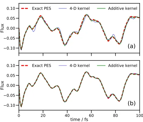
B. Salicylaldimine Proton Transfer
In this section, we present the results of wavefunction propagations performed on a 4-dimensional model of pro-ton transfer in salicylaldimine using a development ver-sion of the Quantics quantum dynamics package71. Three different calculations were performed: (i) a reference SM calculation propagation using the VCHAM-fitted PES of Polyak et al57, (ii) DD-SM on the same PES using a 4-dimensional kernel, and (iii) DD-SM on the same PES using a second-order additive kernel.
All calculations were performed in mass-frequency scaled normal mode coordinates; using the nomenclature of Polyak et al the in-plane modes v1 (proton transfer mode),v13(bending of O and N away from one another), v32 (CO stretch and NH bend) and v36 (OHN bending) were chosen as the system DOFs. A sine DVR of 101 gridpoints was used for the v1 mode whilst 21 member harmonic oscillator DVR bases were used for the other three modes. The initial wavepacket was a 4-dimensional Gaussian function centred at hv1i=0.96 (to the enol side of the barrier),hv13i=hv32i=0 andhv36i=0.14, with widths of hdv1i=0.5706, hdv13i=0.6902, hdv32i=0.6707,
hdv36i=0.7704. Time-propagation was carried out for 100 fs; the DD-SM calculations sampled the PES every 1 fs, with 300 geometries being randomly selected within 3 times the width of the wavepacket from the centre in each DOF. PES values were calculated at the chosen ge-ometries if the variance there was greater than 10−3. A
0.10 0.05 0.00 0.05 0.10
Flux
(a)
Exact PES 4-D kernel Additive kernel0 20 40 60 80 100
time / fs
0.10 0.05 0.00 0.05 0.10
Flux
[image:7.612.318.554.74.275.2](b)
Exact PES 4-D kernel Additive kernelFIG. 1. Flux operator expectation value for a model of sal-icylaldimine with 4 DOFs. The dividing surface is placed at the barrier of the transition mode,v1. Both (a) and (b) show
results of grid-based quantum dynamics using the standard grid method on the fitted PES (red dashed lines), a DD-SM simulation using a 4-dimensional KRR PES (thin blue line), and a DD-SM simulation using a second-order additive kernel (thick green line). In (a), DD-SM results are shown for the initial wavefunction propagation; in (b), DD-SM results are shown for a second simulation in which all reference points learned in (a) are used to construct the respective potential energy operators.
kernel width parameter, α, of 0.5 was used for all DD-SM calculations. Subsequently, DD-DD-SM calculations were performed using the database of energies calculated pre-viously, with the potential energy operator generated at the start of the calculation and with no further enlarge-ment of the initial PES database. In all cases, the EOMs were integrated using the 15th-order short iterative Lanc-zos (SIL) method with accuracy cutoff of 10−6. A flux operator10 was evaluated at q1=0 during the propaga-tion, allowing measurement of the flow of the wavefunc-tion across the potential barrier for the proton transfer.
appearing later on as inaccuracies due to the sampling of the potential creep in.
The key difference in performance between the kernels is in the calculation timings. Both DD-SM calculations employed a single core on a standard desktop machine; however, whilst the full-kernel calculation required 15.5 CPU hours, the additive kernel calculation took 2.25 CPU hours (an improvement by a factor of around 7). The origin of the difference in computational effort is the different number of points added to the database of electronic energies; the full kernel calculation generated 8,026 energies, but the additive kernel only required 741 geometries to be sampled to generate an accurate PES representation. This saving in the number of energy dat-apoints required in the two DD-GB methods accounts for nearly all of the difference in the computation time (in fact, the times required for wavefunction propaga-tion were quite similar, 2,425 against 2,151 CPU seconds for the additive and full kernels, respectively). Further-more, the calculation of the KRR variances and weights took nearly 10,000 CPU seconds with the full kernel, but only 36 CPU seconds with the additive kernel (this huge difference reflects the relative speeds of solving the linear equations in Eqs. (11) and (16) when using a matrix with 100 times fewer entries). Finally, the largest difference in timings was actually in calculating and storing the inte-grals in Eq. (15): 43,700 CPU seconds for the full kernel against 5,300 for the additive kernel. Both calculations used the same size DVR grid, so the difference in these times is solely due to the number of terms in the poten-tial operator. In these calculations, where a pre-fitted, analytic potential is available, the individual energy cal-culations are trivial, but if this calculation were repeated using an ab initio electronic structure program, where each energy calculation can take anything from a few seconds to many minutes or more, the ability to reduce the number of calculations by an order of magnitude will result in a large saving of computational effort.
Figure 1(b) shows results for a second set of DD-SM simulations performed using the full databases generated by the respective full-kernel and additive kernel simula-tions from Fig. 1(a). The agreement between both cal-culations and the exact result is essentially perfect; the improvement of both fits compared to the original cal-culations is to be expected as a much larger region of configuration space has been used to generate the poten-tial energy operator. In this secondary calculation, the time savings for the additive kernel over the full kernel are not as marked as in Fig. 1(a) (2,710 and 3,215 CPU sec-onds for full and additive kernels, respectively), because the computationally-demanding integral evaluation only occurs once, at the start of the propagation.
The conclusion of this section is that we find that the additive kernel is able to reproduce an underlying PES just as accurately as the full kernel, but requires far fewer energy evaluations; this result is very promis-ing for grid-based quantum dynamics. However, initial attempts to combine the additive kernel method with
MCTDH to allow DD-MCTDH simulations did not lead to any significant time-savings. In particular, when us-ing the additive kernel, each database point gives rise to multiple, individual terms in the potential energy oper-ator, one for each term in the summations in Eq. (25) (e.g. ten each in this case); these terms cannot be con-tracted down to a single operator when using MCTDH. As a result, when attempting to use the additive kernel in a DD-MCTDH scheme, the reduction in computational effort for the single-point energy evaluations and solution of the KRR linear equations is still achieved, but we do not gain anything in MCTDH propagation because there is little reduction in the number of terms in the potential energy operator.
In the next section we outline a further improvement which, in combination with the additive kernel, is able to reduce the number of terms in the potential energy operator, thereby allowing a significant speed up in the dynamics calculations, making DD-MCTDH calculations feasible.
IV. METHODOLOGY IMPROVEMENT II: SINGULAR
VALUE DECOMPOSITION OF A GAUSSIAN PES
A. Theory and Implementation
Here, we present a new method of fitting a PES which provides another step in improving the efficiency of the DD-GB methods. Here, the KRR fitting of the PES is relegated to the secondary status of being an efficient sampling method which generates a representation of the PES; we then implement a second transformation from which another, more compact potential energy operator expression can be determined. In particular, we use the idea, demonstrated in Eq. (15), that, when using a DVR basis, we only need to know the value of the potential term at the location of the gridpoint.
To describe this second extension to our DD-GB ap-proach, we assume that we have a KRR PES generated using the additive kernel approach described above. In the setting of our work, this KRR PES would be gener-ated during a DD-GB simulation and the decomposition method described below can be used to accelerate evalu-ation of integrals over the potential energy operator (as required to accelerate MCTDH simulations). This KRR PES, referred to asV0(q), can then be decomposed into a simpler PES representation, appropriate for MCTDH propagation, using the following steps:
1. First, we evaluate the KRR potential energy function, VKRR, at the origin of the coordinate system,0, to set the relative, constant shift for the PES.
2. The KRR potential energy VKRR(q) is evaluated at the location of the DVR gridpoints along one of the DOFs, with all other DOFs remaining atqf = 0. This
the selected mode (including any constant shift in the potential).
3. One-dimensional KRR PES slices along each of the re-maining DOFs are then generated, but with the value of the KRR PES at the origin being subtracted, this time, to avoid over-counting. By this simple procedure we thus have a representation of the KRR PES as a sum of one-dimensional terms, with a single vector of numbers representing the PES along each DOF.
4. To obtain the 2-dimensional terms which couple wavepacket motion between the DOFs, we must fit the difference of the full KRR PES and the one-dimensional terms, between each unique pair of DOFs; in other words, we are fitting to the residual error between representation of the PES using only one-dimensional terms and the full KRR PES.
To achieve this, consider two DOFs, qg and qh, with
the coupling between them written asVgh(qg, qh).
As-suming this function is separable, the integrals over the DVR basis, which appear in the wavefunction propa-gation, are:
hXi(g)Xj(h)|Vgh(qg, qh)|X
(g)
k X
(h)
l i
=hXi(g)|Vgh(qg)|X
(g)
k ihX
(h)
j |V gh(q
h)|X
(h)
l i
≈Vgh(qig)Vgh(qhj)δikδjl
(26)
So, we find that these coupling terms, when evaluated in the DVR basis, are the product of terms on the DVR coordinate grid along the individual DOFs, g and h. We then define the residual function at any point (qi
g, q j
h) on this new, two-dimensional grid as
Vgh(qig, qhj) =VKRR(qgi, qhj)−Vg(qig)−Vh(qhj)
−VKRR(0) (27)
If the DOFs,g andh, containNg andNh DVR
grid-points, respectively, Eq. 27 defines anNg×Nhmatrix,
Vgh, the elements of which are the value of the
resid-ual at each point.
5. We can then decompose the matrix Vgh into a sum of outer products of two vectors, each term of which represents a contribution to the total coupling term. The vectors contain the values of each coupling term at the locations of the DVR gridpoints along the separate DOFs. To find such a set of vectors, we minimize the following squared Frobenius norm,
||Vgh−Vghg ⊗Vhgh||2 (28)
by performing a singular value decomposition (SVD) of the coupling matrix
Vgh=UΣWT (29)
with the singular values in Σbeing in non-decreasing order. It follows that
Vgh(qig, qhj) =
min(Ng,Nh)
X
k=1
σkuikwjk (30)
We can thus set the elements of the required vec-tors, Vgh
g and V
gh
h , which correspond to the values
of the potential energy operator terms at the DVR gridpoints, to be
Vggh(k)(qig) =
√
σkuik (31a)
Vhgh(k)(qhj) =√σkwjk (31b)
6. Finally, we note that, in practice, the term with the largest singular value is added, and then a new resid-ual is created by subtracting this term from the orig-inal. If the norm of this new residual is below some pre-determined accuracy cutoff, no further terms are added; if the norm of the residual is larger than the cutoff, we loop over the other singular values in de-scending order, adding terms and checking the norm of the residual until convergence is reached.
7. The decomposition procedure above is repeated for all pairs of DOFs in the system.
The resulting PES representation is much more com-patible with efficient MCTDH propagation because the multiple potential energy terms of the original KRR PES are contracted down tof one-dimensional terms and at mostPf
g<hmin(Ng, Nh) two-dimensional terms. Finally,
we note that this method has a similar philosophy to the POTFIT algorithm10, which takes a PES evaluated on a grid and produces a PES in sum-of-product form by decomposing PES density matrices. An important sim-ilarity between the methods is that, in the context of grid-based dynamics methods such as MCTDH, the ex-act functional form of the potential is less important than obtaining the values of the potential terms at the loca-tions of the DVR gridpoints. Of course, the underlying KRR PES used in our DD strategies is already in sum-of-products form, albeit with a sum which has too many terms for efficient simulation.
B. Salicylaldimine Proton Transfer: 4D
In this section, we demonstrate the improved computa-tional efficiency of the SVD PES fitting method over the standard KRR approach, whilst simultaneously showing that the new method does not lead to a reduction in ac-curacy in the quantum dynamics.
initial wavefunction and GPR sampling, although we fo-cus here on the second-order additive kernel only. In addition, we also us the same fitted PES as that consid-ered in Section III B. Wavefunction propagation was per-formed using MCTDH with two sets of 14 SPFs each; one describing modesv1andv36, the otherv13andv32. The variable mean field10 implementation of the 6th-order Adams-Bashforth-Moulton (ABM) integrator was used to solve the EOMs with an accuracy parameter of 10−5 and initial step length of 10−4fs. A database of ener-gies was created on-the-fly during propagation, and the SVD procedure, described above, was used to generate the potential energy operator for the dynamics from the KRR fit using the additive kernel. Terms from the SVD fit (Eq. (30)) were added until the Frobenius norm of the residual over all gridpoints was less than 10−3. Following an initial pass in which the PES was generated on-the-fly, a second propagation was then performed using the full database of energies generated previously, with the PES fit performed at the start of the propagation and not updated further.
0 20 40 60 80 100
Time / fs
0.10 0.05 0.00 0.05 0.10
Flux
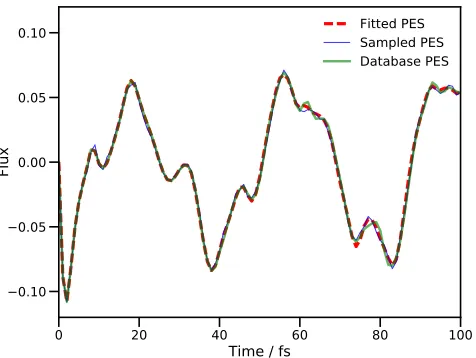
[image:10.612.57.295.329.508.2]Fitted PES Sampled PES Database PES
FIG. 2. Calculated proton transfer flux operator expectation value for a four DOF model of salicylaldimine. The dividing surface is placed at the barrier of the transition mode, v1.
The dashed, red line is the result of using standard MCTDH with the fitted PES. The thin blue line is the result of a DD-MCTDH calculation with the potential energy operator con-structed using SVD/additive kernel, and the thick green line uses the same SVD method, but using the PES database gen-erated in the previous sampling calculation. All simulations used energies evaluated using the fitted PES of Polyaket al.57
In Fig. 2 we present the calculated flux expectation value along thev1mode for both calculations, as well as the result from an MCTDH calculation using the same PES. There is little to say about the results in Fig. 2, except that the DD-MCTDH calculations give results in excellent agreement with the standard MCTDH calcula-tion.
With regards to computational effort, 741 energy val-ues were added to the PES database during the first DD-MCTDH propagation. This calculation took 3,893 CPU seconds on a single-core desktop computer, with the SVD fitting routines contributing only 59 CPU seconds to the total; in other words, the additional effort from SVD fit-ting is minimal. The next question is whether there is a saving in effort given by reducing the number of terms in the potential energy operator. For a one-state, four-DOF problem, there are ten potential terms for each en-ergy value added to the database when using the stan-dard KRR fit with the second-order, additive kernel; in the calculation reported here, this means the potential energy operator without SVD reduction would comprise 7,410 terms.
During the first calculation, when the PES is ini-tially sampled, the number of potential energy opera-tor terms, generated by the new SVD procedure, ranged from 39 to 56 (with a different number generated af-ter each sampling step). The second calculation, using the pcomputed database, used a fit of 56 terms, a re-duction by a factor of more than 130 over the standard KRR fit. It is also worth noting that the VCHAM fit-ted PES, from which we extracfit-ted the energies used in these calculations, had 40 potential operator terms (19 1-dimensional terms and 21 2-dimensional, compared to a split of 4 and 52 in the SVD fit). The SVD fit in this case requires only a few more terms than the VCHAM fit and, in fact, the DD-MCTDH calculation with the pre-computed database took less time than the standard MCTDH calculation (1,222 against 2,098 CPU seconds ) due to shorter integration time-steps being taken in the latter case.
C. Salicylaldimine Proton Transfer: 6D
Having demonstrated the accuracy and reduced putational effort, we provide a further example to com-pare with results from our previous work60. In this previous case, we considered a 6-dimensional model of proton transfer in salicylaldimine, performing MCTDH dynamics using the fitted PES, and the standard KRR fit with full kernel. In that work, we found reasonable agreement between the full, MCTDH dynamics and the DD-MCTDH calculation, but with considerable compu-tational effort. As such, we repeat these calculations here using our new DD-MCTDH scheme to further assess the benefits.
ini-tial wavepacket was the product of Gaussian functions in all six DOFs, with centres and widths as described above for the four original DOFS and, additionally centred at
[image:11.612.57.294.236.415.2]hv10i=hv11i=0.0, with additional widths hdv10i=0.7745 andhdv11i=0.7590.
Figure 3 shows the flux along v1 for three calcula-tions: (i) standard MCTDH using the fitted PES, (ii) DD-MCTDH using the additive kernel and SVD fitting, with a database of energies from a prior calculation, and (iii) DD-MCTDH using the standard, 6-dimensional ker-nel with a pre-computed database of energies and using 18 SPFs per mode, as presented previously in reference 60.
0 20 40 60 80 100
Time / fs
0.10 0.05 0.00 0.05 0.10
Flux
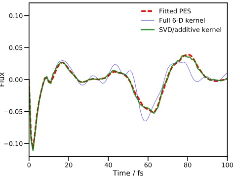
Fitted PES Full 6-D kernel SVD/additive kernel
FIG. 3. Plot of the flux operator expectation value for a six degree-of-freedom model of salicylaldimine. The dividing sur-face is placed at the barrier of the transition mode, v1. The
solid, red line is the result of using MCTDH with the fitted PES. The hashed, blue line is the result of a DD-MCTDH calculation with the potential operator constructed using the SVD fit to an additive kernel GPR PES and the dashed, green line is the equivalent result running the calculation with the pre-calculated database. All calculations used energies calcu-lated from the fitted PES of Polyaket al57.
Figure 3 clearly demonstrates the improvement in agreement between the full MCTDH result and the DD-MCTDH calculations when using the SVD fit and addi-tive kernel; the RMS errors in the calculated fluxes are an order of magnitude smaller when using SVD and additive kernel, compared to the full kernel calculation. We note that the effect of using 14 SPFs per combined mode as opposed to 18 in the full kernel DD-MCTDH calculation is minimal; an 18 SPF MCTDH calculation was also car-ried out and the plot of the flux was found to be almost identical to the corresponding 14 SPF calculation.
The errors in the full kernel case are due to the lack of convergence in the database of energies60; 10,101 en-tries were sampled, the maximum possible in that calcu-lation, and the propagation took 143 hours on 16
proces-sors. As a result, achieving convergence of the database would require a huge additional computational effort. In contrast, the SVD/additive kernel calculation only needed a database of 2,185 energies, once again illustrat-ing the large savillustrat-ing in effort by usillustrat-ing an additive kernel. From these 2,185 energies, a potential expansion of 134 terms was constructed by the SVD procedure, compar-ing very favourably with the 45,885 needed when uscompar-ing the additive kernel alone (six 1-dimensional, and fifteen 2-dimensional, termsper database entry). We also note that the VCHAM-fitted PES contained 78 terms in the six DOFs (29 1-dimensional and 49 2-dimensional), so the DD-MCTDH procedure does require more terms in the PES expansion, leading to a longer propagation (4,451 CPU seconds compared to 3,258 in the standard MCTDH calculation, both on a single processor on a desktop ma-chine). Just over 12 hours CPU time was required for the initial propagation which generated the database for PES construction in the DD-MCTDH calculation, mean-ing that the full DD-MCTDH procedure with SVD and additive kernel took about 13 and a half hours; this is far less computational effort than required to perform ei-ther VCHAM fitting or a DD-MCTDH calculation using the full kernel. We also note that the use of 14 SPFs per combined mode as opposed to 18 for the full kernel calculation produces a saving in effort, all things being equal, but only by a factor of about 2.7 (based upon Eq. (74) in reference 10); nowhere near enough to account for the actual difference, which is mainly down to the size of the database. The use of SVD fitting with addi-tive kernel in DD-MCTDH thus improves accuracy while simultaneously reducing computational effort.
D. Non-Adiabatic Dynamics of Pyrazine
As a final example showing the utility of the pro-posed SVD/additive kernel variant of the DD-MCTDH approach, we present results of a simulation modelling the non-adiabatic dynamics of pyrazine using ab initio electronic structure calculations. Pyrazine is a classic test case in non-adiabatic dynamics, particularly in the calculation of the absorption spectrum obtained by exci-tation to the S2 excited electronic state.15–17. The pres-ence of a conical intersection with the S1 state in the vicinity of the Franck-Condon geometry makes this sys-tem an ideal test of whether a method can accurately represent the wavepacket as it moves between the elec-tronic states.
on the two excited states using the four mass-frequency scaled normal-modes v6a, v10a, v1 and v9a (given as modes 3Ag, 7B1g, 10Ag and 15Agby Molpro), as used in the original MCTDH studies. Harmonic oscillator DVR basis sets were used along all four modes with 32, 22, 21 and 12 functions, respectively, One-dimensional SPFs were used for all DOFs, with different functions on each state (the multi-set formalism10): 7 SPFs on each state were used alongv6a, with 12 on S1and 11 on S2onv10a, 6 and 5 respectively alongv1, and sets of 5 and 4 members each on v9a. The default ABM integrator was used to solve the MCTDH EOMs for 100 fs, with the initial wave-function constructed as a product of thev=0 harmonic oscillator eigenfunctions along each mode, placed on the S2 state and centered at the Franck-Condon point. To generate energies to construct the KRR representation of the PES, 100 points within 3 standard deviations of the wavepacket centre were sampled every femtosecond and added to the database if the variance at that geom-etry exceeded 10−3. The energies of the two electronic states, along with the non-adiabatic couplings between them, were calculated using SA-CAS(8,8)/DZP, as de-scribed above; the energies were diabatised as outlined in Section II A prior to performing KRR fitting. Ad-ditionally, in order to maintain symmetry in the PES, each geometry was reflected in thev6a/v1/v9a plane (i.e. the sign of thev10a coordinate was changed and a point added at the resulting geometry). The additive kernel was used in the KRR process, and the SVD fitting pro-cedure was used to generate the final PES on which the dynamics were performed.
As above, two calculations were performed; the first to generate the database of energies needed to repre-sent the PES, and the second using the full database. Overall, 5,185 energies were generated during the first propagation, resulting in 335 terms in the PES expansion generated using SVD. Results from both calculations are shown in Figs. 4 and 5.
In Fig. 4, we show the absorption spectrum after verti-cal excitation to the S2state, calculated in both calcula-tions using the Fourier transform of the autocorrelation function
c(t) =hΨ(0)|Ψ(t)i. (32)
More details of this method can be found in reference 10, particularly regarding the use of a damping function to minimise artefacts in the spectrum.
Our calculations are not aimed at reproducing the ex-perimental spectrum to a high degree of accuracy; the relatively low-level electronic structure method used to generate the PES precludes such efforts. We note that the original MCTDH studies of pyrazine15–17used a PES which was finely tuned to reproduce the experimental spectrum. Instead, our aim here is to show that a reasonably-accurate absorption spectrum can be calcu-lated (in a reasonable wall-time) using ab initio calcu-lations and our SVD/additive-kernel method. The total wall time for our first calculation was 101 hours
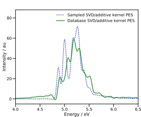
(includ-4.0 4.5 5.0 5.5 6.0 6.5
Energy / eV
0 20 40 60 80
Intensity / au
Sampled SVD/additive kernel PES Database SVD/additive kernel PES
FIG. 4. Absorption spectra of pyrazine after vertical exci-tation to the S2 state. Energies are relative to the S0
min-imum. The blue dashed line is the spectrum obtained in a DD-MCTDH calculation using an additive kernel and SVD fitting of the PES, with energies being added to the database on-the-fly. The green solid line is the spectrum from a DD-MCTDH calculation using the full database of energies gen-erated during the first propagation.
ing all electronic structure calculations) using a single processor on a desktop machine, whilst the second prop-agation took just 612 minutes. Around 88.6% of the first MCTDH calculation time was taken up in evaluating the KRR variance (Eq. (16)); clearly there is a need for im-provement here if possible.
The calculated spectra highlight the need to run an initial calculation (or even perhaps more than one in or-der to build up a converged PES) which samples config-uration space before running a final calculation with a static PES database. The spectrum from the first prop-agation has some unphysical, negative regions (around 4.8 eV) along with tails at high and low energies, suggest-ing a low-accuracy representation of the PES. Further-more, the addition of new energies to the PES database every femtosecond means that the PESs over which the wavepacket is moving are time-dependent, such that en-ergy is not strictly conserved, leading to inaccuracies in the spectrum.
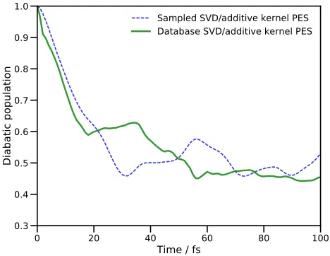
[image:12.612.324.555.60.253.2]used here is not highly-accurate, we are able to reproduce a key feature of the dynamics of pyrazine. The qualita-tive similarities in population transfer follow through the duration of the dynamics; the population reaches a min-imum after 30 fs (after about 45 fs in the earlier work15) before a recurrence peaking after 60 fs (80 fs previously). These similarities indicate that, given further improve-ments in the efficiency in our algorithm, and using a more accurate electronic structure method, the DD-MCTDH method proposed here is capable of producing accurate results in a reasonable time.
0 20 40 60 80 100
Time / fs
0.3 0.4 0.5 0.6 0.7 0.8 0.9 1.0
Diabatic population
[image:13.612.60.294.209.390.2]Sampled SVD/additive kernel PES Database SVD/additive kernel PES
FIG. 5. Population of the second excited diabatic electronic state of pyrazine after vertical excitation. The blue dashed line is the result obtained by a DD-MCTDH calculation us-ing an additive kernel and subsequent SVD fittus-ing of the po-tential with energies being added to the database on-the-fly. The solid green line is the result of a DD-MCTDH calculation using the database of energies generated by the first propa-gation.
V. CONCLUSIONS
We have presented two improvements to our previously published DD method, both of which significantly im-prove the computational efficiency of the method: the use of an additive kernel in KRR greatly reduces the number of electronic structure calculations required to represent the PES, while the SVD fitting procedure can quickly and accurately reduce the number of terms in the result-ing potential energy operator. Our simulations of proton transfer in salicylaldimine and non-adiabatic dynamics in pyrazine show that our method can be used to efficiently model quantum dynamics in many-dimensional systems. That said, further developments are clearly warranted. As mentioned in the discussion of the pyrazine results, calculating KRR variance is a relatively expensive op-eration and should be addressed. Further work on the
choice of the kernel is needed to determine whether an alternative would allow further reductions in the required number of electronic structure calculations. It is also pos-sible to look into optimisation of the parameters in the kernel, particularly the coefficient of the exponent (which determines the width of the Gaussian functions); an opti-mal choice here will again reduce the number of electronic structure calculations needed. The use of gradient infor-mation to improve the representation of the PES is an-other possible avenue of investigation. We are also aware that the structure of a PES is not necessarily limited to interactions between, at most, two DOFs, and interac-tions between three or more DOFs may be required in an accurate expansion of the potential. Extension to in-clude higher-order terms is ongoing, focusing on tensor decomposition to generalise the SVD fitting procedure. Finally, we note that thea priori choice of DOFs to in-clude in the dynamics is an open question which we are aiming to address, particularly when dealing with larger molecules.
However, with the developments proposed here, an on-the-fly implementation of MCTDH, without the arduous task of pre-fitting a sum-of-products potential energy op-erator, is now a reality.
ACKNOWLEDGMENTS
The authors gratefully acknowledge the Leverhulme Trust for funding (RPG- 2016-055) and the Scien-tific Computing Research Technology Platform at the University of Warwick for providing computational re-sources. Data from Figs. 1-5 may be accessed at http://wrap.warwick.ac.uk/id/eprint/98400.
1N. Boekelheide, R. Salom´on-Ferrer, and T. F. Miller III, Proc.
Nat. Acad. Sci. USA108, 16159 (2011).
2L. Masgrau, A. Roujeinikova, L. O. Johannissen, P. Hothi, J.
Bas-ran, K. E. Ranaghan, A. J. Mulholland, M. J. Sutcliffe, N. S.
Scrutton, and D. Leys, Science312, 237 (2006).
3C. T. Middleton, K. de La Harpe, C. Su, Y. K. Law, C. E.
Crespo-Hern´andez, and B. Kohler, Annu. Rev. Phys. Chem.60,
217 (2009).
4V. G. Stavros and J. R. Verlet, Annu. Rev. Phys. Chem.67, 211
(2016).
5L. A. Baker, M. D. Horbury, S. E. Greenough, F. Allais, P. S.
Walsh, S. Habershon, and V. G. Stavros, J. Phys. Chem. Lett.
7, 56 (2016).
6L. A. Baker, S. E. Greenough, and V. G. Stavros, J. Phys. Chem.
Lett.7, 4655 (2016).
7A. H. Zewail, Science242, 1645 (1988).
8A. Douhal, S. K. Kim, and A. H. Zewail, Nature378, 260 (1995).
9A. H. Zewail, J. Phys. Chem. A104, 5660 (2000).
10M. H. Beck, A. J¨ackle, G. A. Worth, and H. D. Meyer, Phys.
Rep.324, 1 (2000).
11M. Schr¨oder, F. Gatti, and H.-D. Meyer, J. Chem. Phys.134,
234307/1 (2011).
12M. Schr¨oder and H.-D. Meyer, J. Chem. Phys. 141, 034116/1
(2014).
13M. Coutino-Neto, A. Viel, and U. Manthe, J. Chem. Phys.121,
9207 (2004).
14K. Sadri, D. Lauvergnat, F. Gatti, and H.-D. Meyer, J. Chem.
15G. Worth, H.-D. Meyer, and L. Cederbaum, J. Chem. Phys.
105, 4412 (1996).
16G. Worth, H.-D. Meyer, and L. Cederbaum, J. Chem. Phys.
109, 3518 (1998).
17A. Raab, G. Worth, H.-D. Meyer, and L. Cederbaum, J. Chem.
Phys.110, 936 (1999).
18S. Neville and G. Worth, J. Chem. Phys.140, 034317/1 (2014).
19T. J. Penfold and G. A. Worth, J. Chem. Phys.131, 064303/1
(2009).
20M. D. H. K¨oppel, I. Baldea, H.-D. Meyer, and P. Szalay, J.
Chem. Phys.117, 2657 (2002).
21H. Wang and M. Thoss, J. Chem. Phys.119, 1289 (2003).
22H. Wang, J. Phys. Chem. A119, 7951 (2015).
23O. Vendrell and H.-D. Meyer, J. Chem. Phys. 134, 044135/1
(2011).
24T. Hammer and U. Manthe, J. Chem. Phys. 134, 224305/1
(2011).
25K. Giri, E. Chapman, C. S. Sanz, and G. Worth, J. Chem. Phys.
135, 044311/1 (2011).
26H. K¨oppel, W. Domcke, and L. S. Cederbaum, Adv. Chem.
Phys.57, 59 (1984).
27L. S. Cederbaum, H. K¨oppel, and W. Domcke, Int. J. Quant.
Chem.15, 251 (1981).
28H.-D. Meyer, F. Gatti, and G. A. Worth, eds.,Multidimensional
quantum dynamics: MCTDH theory and applications (Wiley,
Weinheim, Germany, 2009).
29M. Persico and G. Granucci, Theo. Chem. Acc. 133, 1526/1
(2014).
30G. A. Worth, M. A. Robb, and B. Lasorne, Mol. Phys.106,
2077 (2008).
31J. C. Tully and R. K. Preston, J. Chem. Phys.55, 562 (1971).
32J. C. Tully, J. Chem. Phys.93, 1061 (1990).
33M. Richter, P. Marquetand, J. Gonz´alez-V´azquez, I. Sola, and
L. Gonz´alez, J. Phys. Chem. Lett.3, 3090 (2012).
34M. Richter, P. Marquetand, J. Gonz´alez-V´azquez, I. Sola, and
L. Gonz´alez, J. Chem. Theory Comput.7, 1253 (2011).
35J. C. Tully, Farad. Discuss.110, 407 (1998).
36D. F. Coker, in Computer Simulation in Chemical Physics,
edited by M. P. Allen and D. J. Tildesley (Kluwer Academic, Dordrecht, 1993) pp. 315–377.
37M. S. Topaler, M. D. Hack, T. C. Allison, Y.-P. Liu, S. L. Mielke,
D. W. Schwenke, and D. G. Truhlar, J. Chem. Phys.106, 8699
(1997).
38B. R. Smith, M. J. Bearpark, M. A. Robb, F. Bernardi, and
M. Olivucci, Chem. Phys. Lett.242, 27 (1995).
39M. J. Bearpark, F. Bernardi, M. Olivucci, M. A. Robb, and
B. R. Smith, J. Am. Chem. Soc.118, 5254 (1996).
40R. Mitri´c, J. Petersen, and V. Bonaci´c-Kouteck´y, Phys. Rev. A
79, 053416/1 (2009).
41P. Lisinetskaya and R. Mitri´c, Phys. Rev. A83, 033408/1 (2011).
42M. D. Hack, A. Jasper, Y. L. Volobuev, D. W. Schwenke, and
D. G. Truhlar, J. Phys. Chem. A103, 6309 (1999).
43M. Ben-Nun, J. Quenneville, and T. J. Mart´ınez, J. Phys. Chem.
A104, 5161 (2000).
44M. Ben-Nun and T. J. Mart´ınez, Adv. Chem. Phys.121, 439
(2002).
45H. R. Hudock, B. G. Levine, A. L. Thompson, H. Satzger,
D. Townsend, N. Gador, S. Ullrich, A. Stolow, and T. J.
Mart´ınez, J. Phys. Chem. A111, 8500 (2007).
46T. Mori, W. Glover, M. Schuurman, and T. Mart´ınez, J. Phys.
Chem. A116, 2808 (2012).
47G. Worth and I. Burghardt, Chem. Phys. Lett.368, 502 (2003).
48I. Burghardt, H.-D. Meyer, and L. S. Cederbaum, J. Chem.
Phys.111, 2927 (1999).
49G. Richings, I. Polyak, K. Spinlove, G. Worth, I. Burghardt, and
B. Lasorne, Int. Rev. Phys. Chem.34, 269 (2015).
50G. A. Worth, M. A. Robb, and I. Burghardt, Farad. Discuss.
127, 307 (2004).
51B. Lasorne, M. J. Bearpark, M. A. Robb, and G. A. Worth, J.
Phys. Chem. A112, 13017 (2008).
52B. Lasorne, M. A. Robb, and G. A. Worth, Phys. Chem. Chem.
Phys.9, 3210 (2007).
53D. Mendive-Tapia, B. Lasorne, G. Worth, M. Bearpark, and
M. Robb, Phys. Chem. Chem. Phys.12, 15725 (2010).
54C. Allan, B. Lasorne, G. Worth, and M. Robb, J. Phys. Chem. A
114, 8713 (2010).
55D. Asturiol, B. Lasorne, G. Worth, M. Bearpark, and M. Robb,
Phys. Chem. Chem. Phys.12, 4949 (2010).
56M. Ara´ujo, B. Lasorne, A. Magalhaes, M. Bearpark, and
M. Robb, J. Phys. Chem. A114, 12016 (2010).
57I. Polyak, C. Allan, and G. Worth, J. Chem. Phys.143, 084121/1
(2015).
58M. Vacher, M. J. Bearpark, and M. A. Robb, Theor. Chem. Acc.
135, 187/1 (2016).
59G. Richings and S. Habershon, Chem. Phys. Lett. 683, 228
(2017).
60G. Richings and S. Habershon, J. Chem. Theory Comput. 13,
4012 (2017).
61C. E. Rasmussen and C. K. Williams, Gaussian Processes for
Machine Learning (The MIT Press, Cambridge, Massachusetts,
2006).
62C. Williams, inHandbook of Brain Theory and Neural Networks,
edited by M. Arbib (The MIT Press, Cambridge, Massachusetts, 2002) pp. 466–470.
63A. Bart´ok and G. Cs´anyi, Int. J. Quantum. Chem. 115, 1051
(2015).
64J. P. Alborzpour, D. P. Tew, and S. Habershon, J. Chem. Phys.
145, 174112/1 (2016).
65L. Mones, N. Bernstein, and G. Cs´anyi, J. Chem. Theory
Com-put.12, 5100 (2016).
66J. Quinonero-Candela, C. E. Ramussen, and C. K. I. Williams, in
Large-Scale Kernel Machines, edited by L. Bottou, O. Chapelle,
D. DeCoste, and J. Weston (The MIT Press, Cambridge, Mas-sachusetts, 2007) pp. 203–224.
67D. Duvenaud, H. Nickisch, and C. E. Rasmussen, in Neural
Information Processing Systems Conference (2011).
68K. Chalupka, C. K. Williams, and I. Murray, J. Mach. Learn
Res.14, 333 (2013).
69P. Dirac, Proc. Cambridge Philos. Soc.26, 376 (1930).
70J. Frenkel,Wave Mechanics(Clarendon Press, Oxford, 1934).
71G. Worth, K. Giri, G. Richings, I. Burghardt, M. Beck, A. J¨ackle,
and H.-D. Meyer, “The Quantics Package, Version 1.1,” Tech. Rep. (University of Birmingham, Birmingham, UK, 2016).
72G. Richings and G. Worth, J. Phys. Chem. A119, 12457 (2015).
73G. Richings and G. Worth, Chem. Phys. Lett.683, 606 (2017).
74B. Esry and H. Sadeghpour, Phys. Rev. A68, 042706/1 (2003).
75M. Baer, Chem. Phys. Lett35, 112 (1975).
76H. Rabitz and O. Ali¸s, J. Math. Chem.25, 197 (1999).
77O. Ali¸s and H. Rabitz, J. Math. Chem.29, 127 (2001).
78T.-S. Ho and H. Rabitz, J. Chem. Phys.119, 6433 (2003).
79H.-J. Werner, P. J. Knowles, G. Knizia, F. R. Manby, M. Sch¨utz,
P. Celani, W. Gy¨orffy, D. Kats, T. Korona, R. Lindh,
A. Mitrushenkov, G. Rauhut, K. R. Shamasundar, T. B. Adler, R. D. Amos, A. Bernhardsson, A. Berning, D. L. Cooper, M. J. O. Deegan, A. J. Dobbyn, F. Eckert, E. Goll, C. Hampel, A.
Hessel-mann, G. Hetzer, T. Hrenar, G. Jansen, C. K¨oppl, Y. Liu, A. W.
Lloyd, R. A. Mata, A. J. May, S. J. McNicholas, W. Meyer, M. E. Mura, A. Nicklass, D. P. O’Neill, P. Palmieri, D. Peng,
K. Pfl¨uger, R. Pitzer, M. Reiher, T. Shiozaki, H. Stoll, A. J.
Stone, R. Tarroni, T. Thorsteinsson, and M. Wang, “Molpro,
version 2015.1, a package of ab initio programs,” (2015).
pre-computed potential energy surfaces
Gareth W. Richings1,a)and Scott Habershon1,b)Department of Chemistry and Centre for Scientific Computing, University of Warwick, Coventry, CV4 7AL, UK
We present significant algorithmic improvements to a recently-proposed direct quantum dynamics method, based upon combining well established grid-based quantum dynamics approaches and expansions of the potential energy operator in terms of a weighted sum of Gaussian functions. Specifically, using a sum of low-dimensional Gaussian functions to represent the potential energy surface (PES), combined with a secondary fitting of the PES using singular value decomposition, we show how standard grid-based quantum dynamics methods can be dramatically accelerated without loss of accuracy. This is demonstrated by on-the-fly sim-ulations (using both standard grid-based methods and MCTDH) of both proton transfer on the electronic ground state of salicylaldimine and the non-adiabatic dynamics of pyrazine.
I. INTRODUCTION
Many chemical processes require a quantum-mechanical description to provide the full picture of the molecular dynamics; examples include proton tunnelling in enzyme catalysis1,2, photochemistry of DNA molecules3,4 or plant sunscreens5,6, and other aspects of femtochemistry7–9. The most direct route to performing quantum dynamical simulations is to provide solutions to the nuclear, time-dependent Schr¨odinger equation (TDSE)
i~
∂Ψ (q, t)
∂t = ˆHΨ (q, t), (1) where q is a vector representing the nuclear degrees-of-freedom (DOFs) of the system in question. Once the wavefunction, Ψ(q, t) is known then one can extract any information required about the time-evolution of the sys-tem.
Solution of the TDSE using so-called grid-based meth-ods is now quite standard; here, the wavefunction is ex-panded and evolved on a grid of localised basis functions, regularly distributed through configuration space10. The multi-configuration time-dependent Hartree (MCTDH) method,10–14 a natural extension of grid-based meth-ods which simultaneously employs time-dependent basis functions, has become the de facto gold standard in the area of wavefunction dynamics. MCTDH is capable of treating a few tens of DOFs and converges to the numer-ically exact solution of the TDSE (given a suitable basis of sufficient size). MCTDH has been used to study, for example: the photochemistry of pyrazine15–17, pyrrole18 and benzene19,20. The upper limit on the system size treatable by MCTDH has been extended by the intro-duction of the multi-layer MCTDH method21–24, bring-ing systems of several hundred DOFs into the purview of fully quantum simulations.
a)Electronic mail: [email protected]
b)Electronic mail: [email protected]
However, there remain significant barriers to using grid-based quantum dynamics methods which mean that their more general uptake by wider computational and experimental communities remains low. The key chal-lenge of using grid-based quantum dynamics is the re-quirement that the system Hamiltonian must be fully de-fined before performing wavepacket propagation. First, only a subset of the DOFs of the molecular system are studied to make the dynamics calculation tractable, so one is faced with a choice as to which DOFs might be important; this is an important challenge when encoun-tering a previously-unstudied system. Second, because quantum mechanics is non-local, the global form of the PES must be known prior to performing the dynam-ics. In simulations using grid-based methods such as MCTDH, the global PES is usually determined by fit-ting pre-defined functions to a set of electronic energies calculated at various molecular geometries, for example by using the vibronic-coupling Hamiltonian (VCHAM) method which is based on PES expansion in low-order polynomials18,25–27. This fitting of the PES is an ex-tremely arduous task which must be performed before one can even begin to perform MCTDH simulations; this is the central barrier to making grid-based methods like MCTDH more widely applicable. As an aside, it is worth noting that a similar difficulty can arise for the kinetic energy operator, although this can often be addressed by an appropriate choice of (e.g.rectilinear) coordinates before commencing PES fitting.28