warwick.ac.uk/lib-publications
Manuscript version: Published Version
The version presented in WRAP is the published version (Version of Record).
Persistent WRAP URL:
http://wrap.warwick.ac.uk/110775
How to cite:
The repository item page linked to above, will contain details on accessing citation guidance
from the publisher.
Copyright and reuse:
The Warwick Research Archive Portal (WRAP) makes this work by researchers of the
University of Warwick available open access under the following conditions.
Copyright © and all moral rights to the version of the paper presented here belong to the
individual author(s) and/or other copyright owners. To the extent reasonable and
practicable the material made available in WRAP has been checked for eligibility before
being made available.
Copies of full items can be used for personal research or study, educational, or not-for-profit
purposes without prior permission or charge. Provided that the authors, title and full
bibliographic details are credited, a hyperlink and/or URL is given for the original metadata
page and the content is not changed in any way.
Publisher’s statement:
Please refer to the repository item page, publisher’s statement section, for further
information.
Initial Mass Function Variations Cannot Explain the Ionizing
Spectrum of Low Metallicity Starbursts
E. R. Stanway
1and J. J. Eldridge
21 Physics Deparment, University of Warwick, Gibbet Hill Road, Coventry, CV4 7AL, UK e-mail:[email protected]
2 Department of Physics, University of Auckland, Private Bag 92019, Auckland, New Zealand e-mail:[email protected]
Received 2nd Oct 2018; accepted 8th Nov 2018
ABSTRACT
Aims.Observations of both galaxies in the distant Universe and local starbursts are showing increasing evidence for very hard ionizing spectra that stellar population synthesis models struggle to reproduce. Here we explore the effects of the assumed stellar initial mass function (IMF) on the ionizing photon output of young populations at wavelengths below key ionization energy thresholds.
Methods.We use a custom set of binary population and spectral synthesis (BPASS) models to explore the effects of IMF assumptions as a function of metallicity, IMF slope, upper mass limit, IMF power law break mass and sampling.
Results.We find that while the flux capable of ionizing hydrogen is only weakly dependent on IMF parameters, the photon flux responsible for the He II and O VI lines is far more sensitive to assumptions. In our current models this flux arises primarily from helium and Wolf-Rayet stars which have partially or fully lost their hydrogen envelopes. The timescales for formation and evolution of both Wolf Rayet stars and helium dwarfs, and hence inferred population age, are affected by choice of model IMF. Even the most extreme IMFs cannot reproduce the He II ionizing flux observed in some high redshift galaxies, suggesting a source other than stellar photospheres.
Conclusions.We caution that detailed interpretation of features in an individual galaxy spectrum is inevitably going to be subject to uncertainties in the IMF of its contributing starbursts. We remind the community that the initial mass function is fundamentally a statistical construct, and that stellar population synthesis models are most effective when considering entire galaxy populations rather than individual objects.
Key words.
1. Introduction
Ionizing photons, those emitted at wavelengths shortwards of the hydrogen Lyman Limit at 912Å, have played a key role in shaping the evolution of the intergalactic medium and the galax-ies which form and interact within it. In the local Universe, the emission of such photons originates from a mixture of sources. Amongst these, two are most prominent: sources powered by ac-cretion onto compact objects and supermassive black holes, and the emission from the photospheres of hot, massive stars. In the distant Universe, massive active galactic nuclei (AGN) are rarer. Their number density drops far more rapidly than that of star forming galaxies and hence star formation dominates the ion-izing photon background (Robertson et al. 2015). Lyman con-tinuum (hydrogen-ionizing) photons escaping from star forming galaxies were responsible for the process of ionizing the
inter-galactic medium at redshifts ofz& 6, and also have an
impor-tant impact on the thermal conditions within, and emission spec-tra observed from, the galaxies themselves. As a result there has been strong interest in recent years both in the ways in which ion-izing photons leak from their origin galaxies, and in how these photons are produced in the first place (e.g. Rosdahl et al. 2018; Stanway et al. 2016; Wilkins et al. 2016; Ma et al. 2015, 2016; Nestor et al. 2013).
An important development in this field has been the develop-ment of population synthesis models which account for the
ef-fects of binary interactions on stellar evolution pathways. When these are combined with stellar atmosphere models describing the spectral energy distribution of individual stars, the result-ing spectral synthesis yields predictions that can be compared to the observed spectral properties of stellar populations (Eldridge & Stanway 2009, 2012; Stanway et al. 2016).0 This has led to an increasing recognition of the importance of massive stars in young stellar populations for reionization, twinned with an ap-preciation of the uncertainties in their evolution. In particular, both rotation (Topping & Shull 2015) and stellar multiplicity
(Sana et al. 2012; Eldridge et al. 2017) have a strong effect on
massive star evolution, and the impact of stellar binaries or mul-tiples may be still more important at low metallicities (Moe et al. 2018). Binary star evolution can both boost the ionizing photon flux from a stellar population (Stanway et al. 2016) and extend its lifetime (Stanway et al. 2014; Xiao et al. 2018). Crucially this latter property may allow for increased ionizing photon es-cape fractions, as supernovae from the most massive stars blow channels through the circumstellar and circumgalactic medium, allowing ionizing photon leakage (Rosdahl et al. 2018).
Improved spectroscopy has made analysis of the ionizing spectra of distant galaxies possible in recent years, primarily through study of those ionizing photons reprocessed by nebular gas in the interstellar environment. With the detection of mul-tiple, high signal-to-noise absorption and emission features in
galaxies atz ∼ 2−4 (e.g. Du et al. 2018; Steidel et al. 2016;
Maseda et al. 2017), and even higher redshifts in rare cases (e.g. Stark et al. 2017), it is now possible to construct photoion-ization models which yield insight into the physical conditions in these star-forming systems. While there is always some de-generacy between assumed gas conditions and the spectrum of the ionizing potential, a number of distant systems show evi-dence for the presence of a very hard ionizing radiation field. This is observed both in (rest-frame) optical line ratios such
as [O IIIλ5007Å]/[O IIλ3727Å] or [O IIIλ5007Å]/Hβ λ4681Å,
and directly in the strength of nebular emission lines
includ-ing C III]λ1909Å (which requires a 48 eV ionization potential)
and He IIλ1640Å (at 54.4 eV) in the ultraviolet (Du et al. 2018;
Rigby et al. 2015; Erb et al. 2018, 2010; Berg et al. 2018). Inter-estingly, the class of low redshift extreme emission line galaxies and Lyman-continuum leakers identified as analogues to galax-ies in the distant Universe also show hard ionizing spectra (e.g. Izotov et al. 2018).
Given the association of these hard spectra with intensely star forming galaxies and the absence of clear indications for AGN, a natural question to ask is whether the photospheric
emis-sion from stars can provide sufficient ionizing photons, with
ap-propriate energies. The early indications have indicated mixed answers to this question. While stellar populations including in-teracting binaries have performed well in reproducing the mean properties of galaxies in stacks of high redshift spectra (Steidel et al. 2016), and certainly produce a harder radiation field than a single star population (Eldridge & Stanway 2012; Eldridge et al. 2017; Xiao et al. 2018) and sustain this for significantly longer timescales (Stanway et al. 2014, 2016), reproducing the highest ionization potential lines remains a challenge. In
partic-ular, He II emission (in either the ultravioletλ1640Å or optical
λ4686Å lines) appears to be consistently underestimated given
default stellar population synthesis model assumptions (e.g. Erb et al. 2018; Berg et al. 2018).
Evolutionary population and spectral synthesis - the com-plex process of creating a model spectrum for a stellar system of known age, mass and metallicity based on a combination of individual stellar models - involves a number of approximations and assumptions. At its simplest, it requires a grid of stellar evo-lution models, a grid of stellar atmosphere models to predict ob-servable properties of a star at given temperature and surface gravity, and a function which provides the weighting with which
to combine models of different initial mass. More complex cases
may include evolutionary tracks which include the effects of
stel-lar rotation, Roche-lobe overflow, common envelope and other binary interactions, and expanded grids of atmosphere models which account for surface composition and stellar winds. For the short-lived massive stars that dominate the ionizing spectrum,
the binary fraction is close to unity and the effects of binary
in-teractions can be dramatic (see e.g. De Donder & Vanbeveren 2004; Sana et al. 2012; De Marco & Izzard 2017; Eldridge et al. 2017). Including these pathways, given an assumed set of mass-dependent binary parameter (period, mass ratio) distributions, is thus essential to accurately predict the ionizing spectrum of high redshift galaxies.
However a more fundamental assumption than the binary parameter assumptions is the underlying initial mass function (IMF). This describes the probability distribution of stellar masses (in the binary case, of primary star masses) at zero age
in a starburst, before stellar evolution has any significant effect.
For many years, the assumption of a ‘universal’ mass function has been used to simplify modelling of galaxies. This is usually
described as a power law function in the form dN/dM ∝ Mα
where N is the number of stars in a population at a given mass M
and the function extends between 1 and 100 M. The most
com-monly used prescription, based on that of Salpeter (1955), uses
α=−2.35. However, it has become increasingly clear in recent
years that this oversimplification is untenable. As the extensive reviews in Hopkins (2018) and Kroupa & Jerabkova (2018) dis-cuss in detail, not only is it necessary to break the power law to avoid overpredicting sub-Solar mass stars, but the power law slope at high masses is also highly uncertain. There is evidence for local variations in the IMF and potentially also some
metal-licity dependence. Studies of the massive (M >8 M) and very
massive (M>100 M) star population in the 30 Doradus region
have suggested that the initial mass function in theM >30 M
regime may be as shallow as α = −1.9+0.37
−0.26 (Schneider et al.
2018a,b). Indirect measurements of the initial mass function in the extragalactic regime also suggest a shallow IMF may be ap-propriate (e.g. Wilkins et al. 2008), and similar shallow func-tions have been seen in individual local massive galaxies such as NGC 1399 (Vaughan et al. 2018), while other studies have suggested steeper, ‘bottom heavy’ initial mass functions in ellip-tical galaxies (albeit in the low stellar mass regime, Parikh et al. 2018).
Determining the effects of the plausible range of IMF
varia-tion based on local observavaria-tions is crucial to deciding whether an additional source of hard ionizing photons is necessary to explain the observed results from intense starbursts. A shallow IMF slope will lead to a population that is ‘top-heavy’, i.e. has more massive stars per unit total starburst mass than expected
from a ‘Salpeter’-like slope. A similar, although subtly diff
er-ent, uncertainty arises from the upper mass cut-offin a stellar
population model. While most IMFs do not consider stars with
M >100 M, identification of the very massive star population
in the Large Magellanic Cloud (Crowther et al. 2016) has led
to suggestions that the IMF may extend as far as 300 Min
in-tense starburst regions. Given the dependence of the hard ultra-violet spectrum of a population on its hottest stars, the inclusion or neglect of even a small population of very massive stars can
have a dramatic effect on the photons capable of ionizing not
only hydrogen but also helium. It is thus both timely and nec-essary to explore the photon flux generated above both 13.6 eV and 54.4 eV by young stellar populations, as a function not only of metallicity but also of the assumed initial mass function in a binary stellar population synthesis model.
Is it also instructive to consider the ionizing spectrum at still
higher energies. The far-ultraviolet O VIλ1032,1038Å doublet
(with an ionization potential of 138 eV) is frequently seen in ab-sorption in the halos around low redshift star forming galaxies, and has thus been identified both as sensitive to specific star for-mation rate in galaxies and as a potential tracer of reservoirs of warm ionized gas in the circumgalactic environment (Tumlin-son et al. 2011). In this case the primary ionization source is the extragalactic ionizing background, which is largely powered in turn by emission from active galactic nuclei, while the associa-tion with star formaassocia-tion is provided by the necessity for large scale starburst-driven outflows to account for the density, ve-locity profile and composition of the absorbing gas (e.g. Muza-hid et al. 2015). Indeed ionization powered by accretion onto AGN, whether indirectly through the extragalactic background, or directly through short-duty-cycle bursts of activity within the galaxies in question, can likely account for many low redshift O VI absorption features (e.g. Tripp et al. 2008; Oppenheimer et al. 2018; Nelson et al. 2018).
However there are signs that this interpretation may not
galaxies suggests that ionization by the extragalactic background is strongly disfavoured, and either additional local sources of photoionization or mechanisms such as collisional or shock ex-citation are required (Werk et al. 2016; Turner et al. 2015). Ob-servations at high redshift, where the extragalactic background is softer due to evolution in the AGN luminosity function, again imply additional sources of hard photons or collisional mecha-nisms (Chisholm et al. 2018), while there are also now a handful of examples of intense starbursts which show the ultraviolet O VI
lines inemission(e.g. Hayes et al. 2016).
There is general consensus that photoionization models
driven by emission from hot stars are unable to produce sufficient
photons at these energies to explain observations. Nonetheless, the hints of hard ionizing spectra seen in distant objects suggest that we should not rule out this possibility without exploring the limits of the high mass stellar population given plausible IMF models. While observations of the O VI doublet remain chal-lenging at both high and low redshift, it nonetheless provides a useful metric for the hardness of the ionizing spectrum and so will also be considered here.
In this paper, we use a custom set of binary population and
spectral synthesis models to explore the effects of initial mass
function assumptions on the hard ionizing spectra produced by stellar population synthesis as a function of metallicity. In sec-tion 2 we introduce our methodology. In secsec-tion 3 we explore
the effects of assumed IMF slope and the upper mass cut-offin
the massive star population. In section 4 we introduce a second break in the IMF to shallow slopes at very high mass. In section
5 we attempt to quantify the effects of total starburst mass on
ionizing photon flux. Finally in section 6 we discuss the impli-cations of this study and summarise our conclusions in section 7.
2. Method
2.1. Population Synthesis
The BPASS v2.2 data release (Stanway & Eldridge 2018) in-cludes calculation of results for nine initial mass function pre-scriptions. Of these, one is an unbroken power law and two
fol-low the fol-low mass cut-offprescription of Chabrier (2003) with
different upper mass cut-offs. The remainder comprise three
pairs of broken power law models with an initial mass function
slope of -1.3 between 0.1 and 0.5 M and -2.0, -2.35 or -2.7
between 0.5 Mand an upper mass cut-offof either 100 M or
300 M. Calculating such a range of models already represents
a substantial investment of resources, but nonetheless this sparse
model grid is inadequate to fully explore the effects of initial
mass function on the ionizing spectrum.
In order to make such an exploration tractable we mod-ify the BPASS population synthesis to truncate populations at an age of 1 Gyr. This removes the utility of the models as predictors of old stellar populations and astrophysical transient rates, but does substantially speed up the calculation of
mod-els with different input initial mass function parameters. We
also limit our analysis to a subset of five metallicities, namely
Z =10−5,10−4,0.001,0.010 and 0.020, whereZ
=0.020 is the
metal mass fraction of our Sun. Apart from this, we make no changes to the underlying BPASS v2.2 assumptions (e.g. stellar models, atmosphere models, mass-dependent binary parameters, mass loss rates, mass transfer prescription or synthesis proce-dure).
-2.6 -2.4 -2.2 -2.0 -1.8
High mass slope, αu
0.0 0.2 0.4 0.6 0.8 1.0
Cumulative Fraction of Stellar Mass
300MO •
100MO •
Single
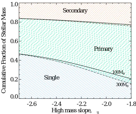
[image:4.595.325.549.67.254.2]Primary Secondary
Fig. 1.The effect of IMF slope on binary star fraction in a population of total mass 106M
, given the stellar mass-dependent binary fractions implemented in BPASS v2.2. The lower region between the x-axis and the first pair of lines indicates the fraction of the total stellar mass for a given IMF slopeαuwhich is assigned to single star models, the central region the mass fraction in primary star models and the upper region the mass fraction assigned to their less massive secondary companions. Regions between each pair of lines (with hatching in two styles) switch between stellar model types depending on the IMF. Models assume a single power law break (αm=αl), The upper cut-offmass,Mu, is shown by line style (100M- solid; 300 - dot-dash). The curves forMu=150 & 200Mlie between these curves.
For the purposes of this analysis we adopt a twice-broken power law for the initial mass function, of the form:
dN(M)
dM =Al Z Ml
M0
MαldM+A m
Z Mm
Ml
MαmdM+A u
Z Mu
Mm
MαudM,
whereαl is the low mass slope between M0 and lower break
mass Ml,αm is the intermediate mass slope valid between Ml
and intermediate break massMmandαuis the upper mass slope
which is effective betweenMmthe upper cut-offmass limitMu.
The constantsAl,AmandAu ensure the function is continuous
and normalised to yield a total population of 106M. In the case
whereαm=αuthe break massMmbecomes arbitrary and the form
collapses to a simple broken power law.
In table 1 we summarise both the standard BPASS IMFs and the parameter ranges explored in this work, according to this for-mulation. In all cases we fix the lower mass limit and power law slope. The stellar binary fraction implemented in BPASS v2.2 is mass-dependent (based on that of Moe & Di Stefano 2017). Hence a consequence of varying the IMF is that the mass frac-tion of single stars versus binaries (primary and secondary mod-els) is also IMF dependent. In figure 1 we show how the single star fraction varies as a function of both IMF slope and upper
mass cut-off. Note that this is independent of metallicity in the
current implementation.
2.2. Ionizing Spectrum parameterisation
We define the photon flux generated by each model as:
Q(X)=
Z λc
1Å
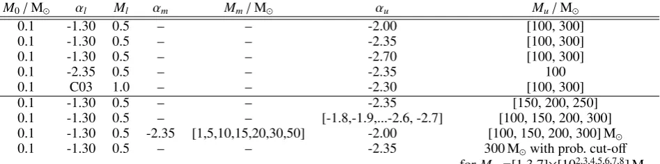
M0/M αl Ml αm Mm/M αu Mu/M
0.1 -1.30 0.5 – – -2.00 [100, 300]
0.1 -1.30 0.5 – – -2.35 [100, 300]
0.1 -1.30 0.5 – – -2.70 [100, 300]
0.1 -2.35 0.5 – – -2.35 100
0.1 C03 1.0 – – -2.30 [100, 300]
0.1 -1.30 0.5 – – -2.35 [150, 200, 250]
0.1 -1.30 0.5 – – [-1.8,-1.9,...-2.6, -2.7] [100, 150, 200, 300]
0.1 -1.30 0.5 -2.35 [1,5,10,15,20,30,50] -2.00 [100, 150, 200, 300] M
0.1 -1.30 0.5 – – -2.35 300 Mwith prob. cut-off
[image:5.595.63.537.55.173.2]forMtot=[1,3,7]×[102,3,4,5,6,7,8] M Table 1.Stellar initial mass functions used in BPASS v2.2 (above line) and the extended parameter grid explored in this work. ‘C03’ indicates an exponential cut-offof the form proposed by Chabrier (2003). The total starburst mass dependent probability cut-offin the final model grid is explained in section 5.
where the critical wavelengthλc=912 Å for Q(H I), 227.9 Å
for Q(He II) and 89.79 Å for Q(O VI), equivalent to the relevant
ionization potentials of 13.6, 54.42 and 138.12 eV respectively. The resultant fluxes are quoted in units of emitted photons per second.
These are calculated at each time step, for each output spec-trum generated by our stellar population synthesis models. We consider photon fluxes rather than directly studying emission or absorption line profiles in the spectra for two reasons:
Firstly, the flux in spectral features associated with these
transitions (e.g. Lyα λ1216Å, Hα λ6563Å, He IIλ1640Å,
He IIλ4686Å, O VIλ1035 AA) is likely to be modified by
ab-sorption and re-emission in the nebular gas surrounding young star forming regions. Interpretation of line strengths thus re-quires an extensive set of assumptions regarding the conditions, covering fraction and composition of the nebular gas screen.
Secondly, we wish to avoid possible uncertainties introduced into stellar absorption lines by the modelling of stellar atmo-spheres for rare subgroups within the stellar population. BPASS implements a custom grid of OB star atmospheres that are re-quired by binary interaction products (Eldridge et al. 2017) and
also the Potsdam Wolf-Rayet (PoWR,1 Sander et al. 2015)
at-mospheres for stripped helium stars. The PoWR models are ex-trapolated to lower metallicities than they were created at, which may lead to overprediction in certain metal lines, and modifica-tion of the detailed strengths of lines in hydrogen and helium. Due to technical constraints, the current version of BPASS also does not make use of the helium dwarf atmospheres generated by Götberg et al. (2017, 2018) and these may have a substantial impact on the strength of some emission lines.
As a result, we opt to report directly the ionizing flux gener-ated by a starburst rather than studying the detailed outputs that result from our spectral synthesis.
3. Effects of IMF Slope and Upper Mass Limit
As shown in table 1, we expand the standard BPASS IMF grid
with power law models with single breaks at 0.5 Mandαm=αu
in the range -1.8 to -2.7 at intervals of 0.1. We calculate each of
these with four possible upper mass cut-offs: 100, 150, 200 and
300 M, and for each of the output spectra calculate the time
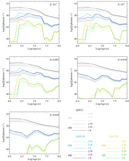
evo-lution of the ionizing photon flux from an instantaneous burst. As figure 2 demonstrates, Q(H I) is largely independent of assumed IMF upper mass limit, and mildly sensitive to the upper mass
1 www.astro.physik.uni-potsdam.de/∼wrh/PoWR/powrgrid1.php
slope, which changes the relative fraction of low mass stars with respect to their massive siblings.
By contrast, Q(He II) shows sensitivity to Mu, particularly
at low metallcity and log(age/years)=6.3-6.5. At these ages very
massive stars are approaching the end of their life, swelling to become very luminous giants and (when stripped by winds or binary interactions) Wolf-Rayet stars. The presence or absence
of these stars is strongly dependent on the upper mass cut-off.
The photon flux shortwards of 89.8Å (138 eV) capable of powering O VI emission and absorption, Q(O VI), is also sensi-tive to the presence or absence of these massive stars, both in terms of the peak flux attained by the population and its tim-ing,as well as to metallicity. Stellar populations including very massive stars produce higher Q(O VI) and at substantially later ages than those which lack very massive stars. At high metal-licities the strong stellar winds exhibited by very massive stars
prevent them from ever becoming sufficiently hot or luminous to
produce a significant Q(O VI) flux.
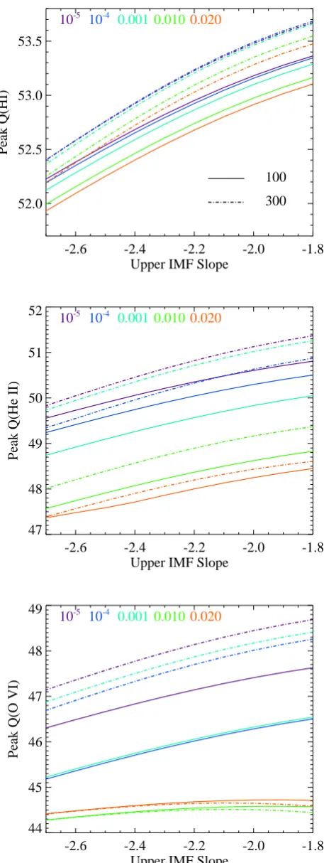
In figure 3 we consider in more detail the effect of
vary-ing metallicity, IMF slope and upper mass limit in each pho-ton flux. Here we show the peak flux obtained by the popula-tion in a given line, which is usually seen in a single time bin
at log(age/years)=6.0-6.5, although we caution that the precise
peak time may vary model by model. The strongest influence on
hydrogen ionizing flux, Q(H I) appears to be the IMF slope,αu.
Over the reasonable range of slopes explored here, peak Q(H I)
varies smoothly by∼ 1.2−1.3 dex at each metallicity
consid-ered. By contrast, peak Q(H I) only varies by∼0.3-0.4 dex when
the slope is fixed and the upper mass limit is altered. Overall, the
range of peak fluxes is confined to a range of log(Q(H I))=
51.9-53.7 for our 106M
populations, narrower than that seen in
Q(He II) and Q(O VI).
While the metallicity dependence of peak values of Q(He II) is perhaps the most visible feature of figure 3 (middle panel), this
flux also shows more dependence on IMF slope (∼1.2-1.6 dex
at fixedMu) than upper mass cut-off(∼0.6-1.2 dex at fixedαu).
The photon flux from the highest metallicity models (Z=0.020)
is both very low and relatively stable to IMF variations.
The IMF dependence of peak Q(O VI) flux is also governed by metallicity. At the lowest metallicities considered here, IMF
slope has a stronger effect than cut-offmass (1.6 dex compared to
0.8 dex). However at intermediate metallicities, around Z=0.001,
the two effects are comparable (∼1.6 dex each). At the higher
metallicities,Z >0.010, the ionizing flux is both very low and
in-6.0 6.5 7.0 7.5 8.0 Log(Age/yr)
40 45 50 55
log(Q/photons s
-1 )
Z=10-5
6.0 6.5 7.0 7.5 8.0
Log(Age/yr) 40
45 50 55
log(Q/photons s
-1 )
Z=10-4
6.0 6.5 7.0 7.5 8.0
Log(Age/yr) 40
45 50 55
log(Q/photons s
-1 )
Z=0.001
6.0 6.5 7.0 7.5 8.0
Log(Age/yr) 40
45 50 55
log(Q/photons s
-1 )
Z=0.010
6.0 6.5 7.0 7.5 8.0
Log(Age/yr) 40
45 50 55
log(Q/photons s
-1 )
Z=0.020
Q(H I)
100 100
-1.8 -1.8 300
300
-1.8 -1.8
-2.35 -2.35
-2.35 -2.35
-2.70 -2.70
-2.70 -2.70
Q(He II)
100 100
-1.8 -1.8
300 300
-1.8 -1.8
-2.35 -2.35 -2.35 -2.35
-2.70 -2.70 -2.70 -2.70
Q(O VI)
100 100
-1.8 -1.8
300 300
-1.8 -1.8
-2.35 -2.35
-2.35 -2.35
-2.70 -2.70
[image:6.595.76.526.66.629.2]-2.70 -2.70
Fig. 2.The time evolution of photon production rates in H I (black), He II (blue) and O VI (yellow-green) at five metallicities, from an instantaneous burst of total mass 106M
occurring at an age of zero. At each metallicity three single-break power law (αu =αm =−1.8,−2.35,−2.70) IMF models are shown at two upper mass limits (Mu =100,300 M), with line style indicating different slopes and line colour different upper mass cut-offs as indicated in the key. The rest of the models lie within the bounds of those shown at fixed age.
dependent of the very massive star population (see e.g. Götberg et al. 2018).
While models with upper mass limitsMu=100 and 300 M
provide the bounding cases at fixed power law slope and
metal-licity, we also consider two intermediate upper mass cut-offs at
Mu =150 and 200 M. We show the variation in peak fluxes as
a function of upper mass limit and metallicity for a fixed IMF
slope (αm = αu = −2.35) in figure 4. The peak H I ionizing
flux increases smoothly with upper mass cut-offat all
-2.6 -2.4 -2.2 -2.0 -1.8 Upper IMF Slope
52.0 52.5 53.0 53.5
Peak Q(HI)
10-5 10-4 0.0010.010 0.020
100
300
-2.6 -2.4 -2.2 -2.0 -1.8
Upper IMF Slope 47
48 49 50 51 52
Peak Q(He II)
10-5 10-4 0.0010.010 0.020
-2.6 -2.4 -2.2 -2.0 -1.8
Upper IMF Slope 44
45 46 47 48 49
Peak Q(O VI)
[image:7.595.56.285.66.674.2]10-5 10-4 0.0010.010 0.020
Fig. 3.The peak ionizing photon fluxes reached by an ageing instan-taneous starburst of total mass 106M
as a function of IMF slope (as-sumingαm=αu). In each panel, metallicity is indicated by colour while upper mass cut-offMuis indicated by line style (100 M=solid, 300 M
=dot-dash).
peak He II flux and O VI flux but anomalous behaviour emerges
in our models withZ ∼ 0.001. At this metallicity (5% of
So-lar) there is a very strong dependence of hard ionizing flux on upper mass limit which results from a combination of physical
effects. These models have sufficient metal line opacities in their
stellar atmospheres to drive mass loss through stellar winds, but
at rates sufficiently low to allow angular momentum to be
re-tained and rotational mixing to strongly influence the evolution of stars. In BPASS models, this chemically homogenous evolu-tion is deemed to occur if significant mass is accreted by stars
withZ<0.004 andM >20 M. The result is that where the
up-per mass cut-offis as low as 100 Mthe majority of massive stars
quickly drop below the BPASS mass limit for onset of chem-ically homogenous evolution and very few rotationally mixed
stars are formed in our models. By contrast, whenMu=300 M
a reasonable amount of mass loss can occur through winds, while
still leaving stars with sufficient mass for rotational mixing to
in-fluence their evolution. Since chemically homogenous stars tend to burn hotter and for longer than a non-rotating star of com-parable mass, these stars dominate emission at wavelengths ca-pable of ionizing He II. The result is a strong dependence on
Mu in the hard ionizing flux atZ = 0.001 relative to those at
higher metallicities (where stellar winds always dominate and fewer stars are stripped) and those at the lowest metallicities.
AtZ ≤ 10−4, stellar winds are very weak due to the low metal
ion opacities in the stellar atmospheres, and very little of the initial stellar mass is lost to winds. These stars are more likely than those at higher metallicities to be rotationally mixed, but those at the lowest metallicity also tend to become inflated to larger stellar radii which increases the probability that their at-mospheres may become stripped by a binary companion (and so again create a hot, blue spectrum). The detailed balance of these
different physical mechanisms for producing hot stars leads to
a somewhat counterintuitive inversion in the metallicity trends
of Q(He II) and Q(O VI) with theZ =0.001 models producing
more hard ionizing photons than those atZ=10−4.
4. Introducing a Second Break
Studies of high mass star forming regions in the local Universe, notably the 30 Doradus complex in the Large Magellanic Cloud, have suggested that the initial mass function for massive stars may be substantially shallower than the Salpeter-like initial mass function that appears common for near-Solar mass stars (Schnei-der et al. 2018a,b). A possible interpretation of these findings is that the power-law initial mass function may show a second break in the high- to very-high-mass regime.
To explore the effects of such an IMF, we calculate a limited
set of models with two power law breaks. We fixM0 =0.5 M,
Mu=300 M,αl = −1.3,αm = −2.35 andαu = −2.0 for
con-sistency with constraints from local studies, while allowing the
intermediate break mass,Mm, to vary. Again, we look at the peak
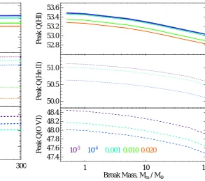
photon fluxes attained by the population as a function of metal-licity, and break mass, as shown in figure 5.
Unsurprisingly, the effects of introducing a second break on
peak photon flux are relatively minor. The model fluxes lie be-tween those of single-break power law initial mass functions
with slopes ofαm=αu =−2.0 and−2.35, tending towards one
or the other depending on the intermediate break mass,Mm
52.4 52.6 52.8 53.0 53.2
Peak Q(HI)
48 49 50
Peak Q(He II)
100 150 200 250 300
Upper Mass Cutoff, Mu / MO • 46
47 48
Peak Q(O VI)
Z=10-5 10-4
[image:8.595.255.549.54.314.2]0.002 0.010 0.020
Fig. 4.The peak ionizing fluxes, colour coded by metallicity, as in fig-ure 3, but now for single-break power law initial mass functions with a varying upper mass limit, Mu. We fixαm = αl = −2.35. The high metallicity fluxes in the He II and O VI ionizing photons are too low to show here, but follow a similar trend.
5. Effects of Total Stellar Mass
BPASS, in common with most other stellar population synthesis
models, assumes that the star forming population is sufficiently
massive that the IMF is fully sampled. An obvious problem with this assumption arises in the case of small starbursts; if the total
mass of a newborn stellar population is only 1000 M, the
prob-ability of forming a single 300 M star is very low. The fully
sampled statistical IMF approach is equivalent to assigning frac-tions of the flux of such very massive stars to the composite spec-trum, rather than considering a binary probability (1 or 0) that the star contributes. Since even a single individual massive star can dominate the hard ionizing radiation from a population, and the spectrum of that star is strongly mass dependent, this presents a challenge to modelling.
An alternate approach is stochastic sampling - drawing in-dividual stars from an underlying probability distribution until the desired total mass is reached (Cerviño 2013). Because this is fundamentally probabilistic, many iterations must be performed for each initial mass function and each total mass under con-sideration, in order to form a complete picture. While models which do this exist and have been used to explore the properties of the ultraviolet continuum (e.g. Cerviño et al. 2003; Pflamm-Altenburg et al. 2009; Villaverde et al. 2010; Fumagalli et al. 2011; Fouesneau et al. 2012; Vidal-García et al. 2017; Paalvast & Brinchmann 2017; Ashworth et al. 2018), these have been limited to treatment of single star populations. A detailed stel-lar evolution-based code such as BPASS is ill-suited for such a procedure. Reading each stellar model in turn, matching it with an atmosphere model at each timestep and calculating its contri-bution to the composite spectrum in a given time bin is a slow process which does not lend itself to many iterations or large grids of parameters. Experimentation with an earlier BPASS
ver-sion suggested that the effects of binary interactions broaden the
50.0 50.5 51.0
Peak Q(He II)
1 10 100
Break Mass, Mm / MO • 47.4
47.6 47.8 48.0 48.2 48.4
Peak Q(O VI)
52.8 53.0 53.2 53.4 53.6
Peak Q(HI)
10-5 10-4 0.001 0.0100.020
Fig. 5.The peak ionizing fluxes, as in figure 3, but now for power law initial mass functions with two breaks. We fix M0 = 0.5 M,
Mu=300 M,αl = −1.3,αm =−2.35 andαu =−2.0, while allowing the intermediate break mass,Mm, to vary. The high metallicity fluxes in the He II and O VI ionizing photons are too low to show here, but follow the same trend.
range of evolutionary pathways at each initial mass and allow for stars to become more massive via mass transfer and mergers
that mitigate some of the stochastic sampling effects (Eldridge
2012).
Here we consider an intermediate approach between sim-ple IMF weighting and full stochastic sampling. For a selected
metallicity (Z=0.001), upper IMF slope (αm=αu=−2.35) and
nominal mass cut-off(Mu=300 M), we consider hybrid initial
mass functions in which the weighting distribution for individual models is generated assuming full sampling but then modified. Given a range of assumed total stellar masses ranging from 100
to 108M
, we remove individual models from the spectral
syn-thesis if their contribution to a stellar population of that initial mass is less than 0.5 stars. We then readjust the overall scaling to account for the diminished mass of stars contributing, giving the final results as the peak photon flux per stellar mass formed in the initial starburst.
In the case of a single star population, in which the probabil-ity of a model occurring only depends on the stellar initial mass,
this approach is equivalent to an upper mass cut-off, Mu, that
scales with the total starburst size. As a binary population syn-thesis code, BPASS includes a large number of models at each initial mass, with weightings which also scale with the (primary mass-dependent) period and mass ratio distributions. As a re-sult, while the highest mass stars will always be excluded from a small population, some intermediate mass primaries will be rep-resented by a subset of period and mass ratio models, while less frequently occurring models will be omitted.
[image:8.595.57.447.56.311.2]102
103
104
105
106
107
108
Total Mass of Starburst / Msun 38
40 42 44 46
Peak Q per Solar Mass
Q(H I)
Q(He II)
[image:9.595.54.286.64.260.2]Q(O VI)
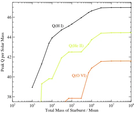
Fig. 6.The peak ionizing photon fluxes per Solar mass of stars, reached by an ageing instantaneous starburst atZ=0.001 as a function of initial total mass assuming a total-mass-dependent cut-off in the high mass stellar population as described in section 5.
low mass population will host a large number of massive stars; in the majority of cases it will not. Similarly it is possible for a high mass starburst to lack any high mass stars when stochastic sampling is taken into acount. Thus the models calculated here are indicative of the scale of the uncertainties rather than their spread.
The results of this analysis are shown in figure 6. As the fig-ure indicates, the ionizing flux from a population does not
be-come a simple product of total stellar mass untilMtotal≥106M,
at which point the IMF is fully populated. The Q(He II) and Q(O VI) flux from BPASS models show plateaus at intermediate masses. This is likely a modelling artifact resulting from the rel-atively coarse grid of BPASS stellar models at high masses, and emphasizing the importance of individual very massive stars in producing these lines. The transition between the ionizing pho-ton flux from a population hosting no very massive stars to one
hosting even a single 300 Mstar is abrupt and dramatic in this
implementation. As a result, it seems likely that stochastic sam-pling of the initial mass function may be important for inter-pretation of high ionization potential spectral features, even in the galaxy-wide starbursts seen in the distant Universe. This has been seen before in work exploring spectral synthesis with sin-gle star evolution models (e.g. Vidal-García et al. 2017; Paalvast & Brinchmann 2017) but the analysis here suggests that the re-sult holds true for binary models, despite the increased range of evolutionary pathways: the ionizing flux of the most massive star is simply too dominant in contributing the hard ionizing photons under consideration.
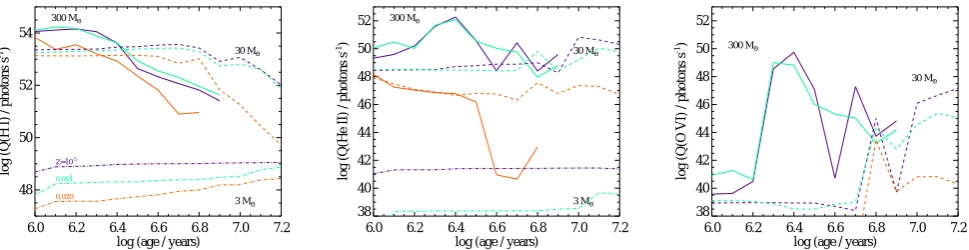
To test the limits of stochastic sampling, we generate three
additional population synthesis models. In the first, only 300 M
primary stars and their binary companions (given by the stan-dard BPASS v2.2 binary parameter distribution) are included in
a population of total mass 106M, in the second, only 30 M
stars (and their companions) and in the third, only 3 M stars
(single and primary, with their binary companions). The ioniz-ing fluxes from these three models as a function of metallicity
are shown in figure 7. The short lifetimes of the 300 M stars
and their rapid evolution leads to extreme variation on their hard ionizing flux in short timescales, even while the Q(H I) hydrogen
ionizing flux declines slowly and smoothly. Stars at 30 Mhave
hydrogen ionizing fluxes almost an order of magnitude lower than the very massive stars, but this is sustained over a much longer lifetime, as is Q(He II). The only photons capable of ion-izing O VI from this population arise from the stripped binary
products present at relatively late times. Finally, the 3 M
pop-ulation produces very little flux shortwards of the Lyman limit, and negligible emission in Q(O VI). All stellar populations show
much lower ionizing fluxes at Solar metallicity (Z=0.020) than at
lower metallicities. The lowest ratio in Q(H I)/Q(He II) attained
by the 300 Mpopulation atZ=10−5is 1.3 dex.
6. Discussion
The range of variation in peak fluxes, given our grid of ‘rea-sonable’ initial mass function parameters is shown in figure 8 at each metallicity, where the values are shown relative to the BPASS default IMF model, which is a power law with a single
break at Ml = 0.5 M,αm = αl = −2.35 and Mu = 300 M.
As the figure makes clear, the hydrogen ionizing fluxQ(H I) is
relatively predictable in its response to IMF variations, as the ef-fect of the IMF is almost independent of metallicity - in other words, if a value is calculated for one IMF and metallicity, the
photon flux given different assumptions can be approximated by
application of a simple scaling factor. By contrast, the hard ioniz-ing flux is far more sensitive to variations in initial mass function and metallicity. In all cases, the default, Salpeter-like upper mass
slope, model lies in the centre of the range ofαlvariations, but
our default cut-offMu=300 Mat the top end of the upper mass
limit variations. At moderate metallicities (Z=10−4−0.010), it
is the upper mass cut-off that has the strongest effect on hard
ionizing flux; very massive stars with M> 100 M are critical
for the production of photons sufficiently strong to power He II
or O VI spectral features. The introduction of a second break to a shallower slope at high masses can also boost hard photon pro-duction by the same mechanism: increasing the number of very massive stars in the population.
While the peak fluxes attained by a population may be criti-cal for interpreting some of the hardest observed spectra in both the distant and local Universe, for the majority of star forming regions, this is attained only for a very brief interval in the star-bursts’ evolution. A more generally useful quantity may be the time-averaged photon flux over the first 20 Myr of stellar
evolu-tion (i.e. at log(age/years)<7.3). As figure 2 demonstrated, this
interval is sufficient to capture the lifetimes of the most
mas-sive stars, and hence the interval in which hard fluxes might be expected. In figure 9 we show the equivalent variation in this quantity. As might be expected, it shows very similar trends to those seen in the peak fluxes, but with the variation mitigated by the time average, yielding somewhat narrower ranges.
6.0 6.2 6.4 6.6 6.8 7.0 7.2 log (age / years)
48 50 52 54
log (Q(H I) / photons s
-1)
Z=10-5
0.001
0.020
3 MO •
300 MO •
30 MO •
6.0 6.2 6.4 6.6 6.8 7.0 7.2 log (age / years)
38 40 42 44 46 48 50 52
log (Q(He II) / photons s
-1)
3 MO •
300 MO •
30 MO •
6.0 6.2 6.4 6.6 6.8 7.0 7.2 log (age / years)
38 40 42 44 46 48 50 52
log (Q(O VI) / photons s
-1) 300 MO •
[image:10.595.61.546.63.188.2]30 MO •
Fig. 7.The ionizing photon flux time evolution for stellar populations comprised entirely of single stars or primaries at a given mass (3, 30 or 300 M) and appropriate binary companions. Three metallicities are shown for each mass, and each energy threshold. For Q(O VI) the emission from low mass and high metallicity stars is negligible.
-1.5 -1.0 -0.5 0.0 0.5 1.0
Maximum Variation in log(Peak Q)
10-5 10-4 0.001 0.010 -1.8 -1.9 -2.0 -2.1 -2.2 -2.3 -2.4 -2.5 -2.6 -2.7 100 150 200 300 0.5 5 20 50 300 0.020
Q(H I) Q(He II) Q(O VI)
αU Mu Mm αU
Mu
Mm αU
Mu
[image:10.595.42.291.250.427.2]Mm
Fig. 8. The range of variation in peak ionizing photon fluxes across the grid of models considered here. Range is shown separately for each metallicity, first for single-break IMFs withMu =300 Mand varying
αm = αl, then for models with fixedαm = αl = −2.35 and varying Mu, and finally for double break models withαm =−2.35,αl =−2.00 and Mu = 300 Mbut varying Mm. All ranges are shown relative to the BPASS default IMF model, which is a single break power law with αm=αl=−2.35 andMu=300 M.
-1.5 -1.0 -0.5 0.0 0.5 1.0
Maximum Variation in log( Mean Q)
10-5 10-4 0.001 0.010 -1.8 -1.9 -2.0 -2.1 -2.2 -2.3 -2.4 -2.5 -2.6 -2.7 100 300 0.5 5 20 50 300 0.020
Q(H I) Q(He II) Q(O VI)
αU Mu Mm αU Mu Mm αU
Mu
Mm
Fig. 9.As in figure 8, but now considering the mean photon flux aver-aged over the first 20 Myr of the starbursts’ evolution.
However, an examination of the right-hand panel of figure 10 suggests that care should be taken in such interpretation. A high metallicity starburst will generate as many, or even more, Wolf-Rayet stars as one that is near-primordial, while showing very
little hard ionizing flux. In fact, atZ =0.020 (Solar metallicity),
the entirety of the high energy flux arises from the more numer-ous but far less luminnumer-ous helium dwarf population generated by binary interactions of intermediate mass stars.
[image:10.595.41.291.534.712.2]However, while Solar-metallicity Wolf-Rayet stars are more numerous, they are also substantially less luminous than their counterparts at low metallicities. The weak stellar winds asso-ciated with low photospheric metal fractions lead to low metal-licity stars retaining much of their mass through their evolution which leads to higher core temperatures to achieve hydrostatic equilibrium and thus higher stellar luminosities. For stars that accrete material through binary mass transfer, the weaker wind mass loss also allows these stars to retain more angular mo-mentum and so they experience strong rotational mixing that causes chemically homogenous evolution to occur. These stars have high surface temperatures for their entire hydrogen-burning lifetimes and contribute significantly to the ionizing flux. The factors all result is much higher luminosities.
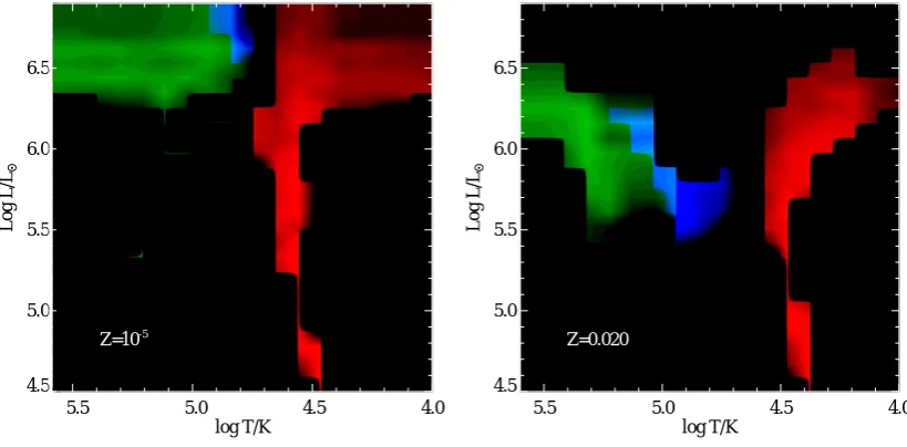
Figure 11 illustrates this with a traditional Hertzsprung-Russell diagram, indicating the luminosity and tempera-ture distribution of stars at the hard emission peak age of
log(age/years)=6.4, as a function of their surface hydrogen mass
fraction. The fraction of partially-stripped stars is higher, and the
individual stars typically∼0.5 dex more luminous, atZ =10−5
than atZ =0.020. At the same time, the metal abundance in the
photospheres is lower. As a result, the spectrum of such starburst populations may be expected to produce substantially weaker traditional "Wolf-Rayet" spectral features (dominated by wind-broadened helium and carbon lines), while still being significant sources of hard ionizing photons. It is unclear whether the Wolf-Rayet atmosphere models currently in use for spectral synthesis fully capture this behaviour at low metallicities.
As we have demonstrated, IMF variations can substantially
affect the ionizing flux. It is interesting to note, however, that
the variations in the ionizing spectrum are somewhat mitigated by the fact that the entire spectrum is responding in a similar way to initial mass function. As figure 12 illustrates, even the most extreme ionizing populations in the grid we have calculated
reach peak Q(He II)/Q(H I) ratios (i.e. spectral hardness
43 45 47 49
log Q(OVI)
6.0 6.5 7.0 7.5 8.0
Log(Age/yr) 1
10 100
Number of Helium Stars
Z=10-5
log L / LO • > 4.9
log L / LO • < 4.9 WN
WNH
WC
43 45 47 49
6.0 6.5 7.0 7.5 8.0
Log(Age/yr) 1
10 100 1000
Z=0.020
log L / LO • > 4.9
log L / LO • < 4.9 WN
WNH
[image:11.595.70.525.58.247.2]WC
Fig. 10.The population of stars with a surface hydrogen mass fraction of Xsurf < 0.4, i.e. helium stars, as a function of time assuming an initial population of 106M
, compared to the photon flux Q(O VI). Those with very low hydrogen (Xsurf <0.001, classic Wolf-Rayet stars) are subdivided by the presence (WC) or absence (WN) of carbon. The population is further subdivided into high luminosity (solid lines) and low luminosity (dot-dash) populations. We show results at the highest and lowest metallicities considered here.
5.5 5.0 4.5 4.0
log T/K 4.5
5.0 5.5 6.0 6.5
Log L/L
O
•
Z=10-5
5.5 5.0 4.5 4.0
log T/K 4.5
5.0 5.5 6.0 6.5
Log L/L
O
•
Z=0.020
Fig. 11.The Herzsprung-Russell diagram for stellar populations at a log(age/years)=6.4, shown at high and low metallicity. Red regions indicate stars with a surface hydrogen mass fraction ofXsurf >0.4, blue those withXsurf <0.001, and green helium stars with an intermediate surface hydrogen fraction. The same density scaling has been applied to both metallicities. Although the number of hot stars is comparable atZ =0.020 toZ=10−5, each star is substantially less luminous than its low metallicity counterpart.
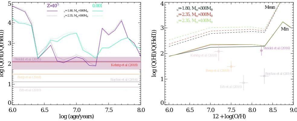
This presents a challenge. The increasing sample of ioniz-ing galaxies in the literature showioniz-ing evidence for a hard ion-izing photon spectrum motivated this study and constraints on the spectral properties of these sources are also shown in figure 12. We have restricted our analysis to a representatitive sample
of extreme sources with measurements of both the Hβ and He II
1640Å or 4686Å recombination lines. While other lines, includ-ing [C IV] 1540, C III] 1909 and O III] 1665 are also indicative of hard ionizing fields, they are also highly sensitive to nebu-lar gas conditions complicating interpretation of line strength. By contrast, the recombination lines of hydrogen and helium are only weakly sensitive to electron density and temperature, such that,
Q(H I)
Q(He II) =
FHλH FHeλHe
αH B αH
eff
αHe
eff
αHe B
,
whereFX andλX are the (extinction and lensing corrected) flux
and wavelength of the lines used,αX
B are the case B
recombina-tion coefficients andαXeff are the effective recombination coeffi
-cients relevant to each specific line. For the observational data
in figure 12 we calculate αXB andαXeff for Ne = 103cm−3 and
Te =15,000 K, using a simple linear interpolation between the
values given by Osterbrock & Ferland (2006) for each line. The electron density and temperature of extreme ionizing sources ap-pear to vary from source to source, from region to region and
even between different tracers from species to species within a
source. The electron density and temperature assumed here is
motivated by observations of SL2S J021737-051329 atz =1.8
(Berg et al. 2018) and by the mean properties of stackedz∼2.3
Lyman break galaxies (Steidel et al. 2016). They may be slightly
higher than are appropriate for Q2343-BX418 (z = 2.3, Erb
[image:11.595.95.505.307.509.2]et al. 2014), but the inferred values for Q(H I)/Q(He II) are only
weakly dependent on this. For SBS 0335-052E (D = 54 Mpc,
Kehrig et al. 2018) we use the values provided by the authors in their table 1 for both the range of ratios in spatially resolved re-gions (shown as a shaded region) and the integrated value for the whole galaxy (shown by a line). Where the observational uncer-tainties on line flux are small, we apply a minimum uncertainty in the photon flux ratio of 0.2 dex, accounting for the possible
effects of extinction, lensing corrections and uncertainty on the
recombination coefficients. None of these sources show any
sig-nificant evidence for AGN activity.
As the figure makes clear, even our most extreme physically-motivated IMF stellar population synthesis models are unable to reproduce the high line ratios (and hence inferred photon flux ratios) observed in some of the most extreme known systems at either high or low redshift. Although the highest flux ratios reached by our models may be consistent with the observational
data for SBS 0335-052E and thez ∼ 2.3 Lyman break galaxy
stack, these will only be attained for brief periods, or at the very lowest metallicities we consider. If the mean ratio observed over a 20 Myr period is considered instead, the requirement for excep-tionally low metallicities (inconsistent with the observed
nebu-lar gas) becomes still stronger. For other objects at z ∼ 2−4,
BPASS stellar spectrum models are simply unable to reproduce the line ratios, regardless of assumed IMF. Indeed, even a
popu-lation comprised entirely of 300 Mstars and their binary
com-panions never drops below Q(H I)/Q(He II)=1.3, given our
stel-lar evolution and atmosphere prescriptions. Hence a stochastic IMF sampling heavy in very massive stars cannot reproduce the observational data. This strongly implies that additional sources of hard ionizing photons need to be considered when analysing highly ionized galaxies, either in the local Universe or at high redshift. It is likely that the source of these hard ionizing photons arises from accretion around compact objects. The open question is whether it arises from acretion onto neutron stars and stellar mass black holes in X-ray binaries (Mirabel et al. 2011; Justham & Schawinski 2012) or supermassive black holes at the center of galaxies acting as AGN Netzer (2015), neither of which are currently included within the BPASS models.
This analysis has necessarily focussed on the output of just one stellar evolution and population synthesis code, the assump-tions and methodology of which have been clearly described in the literature. However given the range of such models in the literature, it is appropriate to consider whether an alternate choice of stellar population synthesis model might yield a dif-ferent conclusion. All model sets face two key questions: which stellar evolution tracks to employ, and what stellar atmosphere models to match them to. The former question includes un-certainties such as the impact of binary evolution or rotation, while the latter incorporates our uncertainty regarding
radia-tive transfer through stellar envelopes as well as the difficulty
of testing or calibrating predictions for the extreme ultraviolet
(which is effectively unobservable due to line-of-sight
absorp-tion by interstellar hydrogen). The degree of uncertainty in the extreme ultraviolet emission of a population even at a main se-quence age of 1 Myr is demonstrated in figure 13. As the figure demonstrates BPASS models produce substantially more ioniz-ing flux than the older Starburst99 (Geneva, non-rotationiz-ing, Lei-therer et al. 1999, 2011) and BC03 (galaxev, Bruzual & Char-lot 2003) population synthesis model at Solar metallicity. The 2016 release of the BC03 models presents a mixed picture. Both when using a BaSeL stellar atmosphere grid, and when using the semi-empirical MILES stellar spectra grid, the BC03-2016 model spectra extend to shorter wavelengths than BPASS at
So-lar metallicity, but the flux normalisation in the ionizing regime appears to be strongly dependent on the stellar atmosphere li-brary in use, with the MILES lili-brary producing a calibration similar to BPASS just below the Lyman limit but failing to match the flux predicted by both BPASS and Starburst99 between 912 and 1216 Å, and exceeding both shortwards of 500Å. The ori-gin of the very blue spectrum at Solar metallicity in the BC03-2016 models is unclear (the details of implementation in this code have not appeared in the literature) but is likely associated with a boost in the number or luminosity of Wolf-Rayet spectra incorporated by the population synthesis. The same trends are
seen at lower metallicities. AtZ =10−4the extreme ultraviolet
spectrum is unconstrained by observations, and the implemen-tation favoured by BC03-2016 is significantly bluer than that of BPASS for the same input IMF. The only other SPS model which is available at this very low metallicity is the Yggdrasil model of
(Zackrisson et al. 2011) which hasZ = 4×10⁻⁴. This is very
similar to theZ =10−4model of BC03-2016 longwards of the
Lyman limit, but more similar to BPASS below it and deficient
in photons withλ <500 Å.
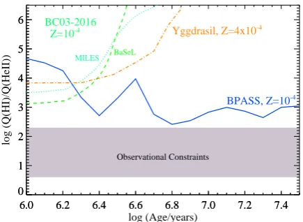
However, as figure 14 demonstrates, the behaviour of the
SPS models at effectively zero age may not be the key
diag-nostic in interpreting the spectra of high redshift stellar pop-ulations. Both the low metallicity BC03-2016 models and the Yggdrasil models evolve rapidly, with strong Q(He II) emission fading away within 2-3 Myr after the stars are formed. By con-trast, binary evolution pathways generate more hot stars at later ages, and as a result the BPASS models maintain strong Q(He II) emission relative to Q(H I) over timescales of 30 Myr or longer. While all the models fail to match the values inferred from the observational constraints, timescale arguments suggest that we
are unlikely to be catching so many systems at ages< 3 Myr,
somewhat favouring the binary evolution models.
7. Conclusions
Our main conclusions can be summarised as follows:
1. Young starbursts at low metallicity can generate the high en-ergy photons (shortwards of 228Å and 89.8 Å) required to power emission or absorption features in the He II and O VI lines.
2. The photon flux at these energies is 2.5 orders of magnitude lower than that shortwards of 912Å for Q(He II), and five orders of magnitude lower for Q(O VI), even when at its peak and at very low metallicities.
3. Hard ionizing radiation, particularly Q(O VI), is associated
with the most massive stars in the population (M >100 M),
and so is short-lived and boosted by shallower power law
initial mass functions or higher mass IMF cut-offs.
4. The probability of these very massive stars occurring in a
starburst with a low total mass is<<1, meaning the fluxes
in Q(He II) and Q(O VI) are highly susceptible to stochastic variation, even in galaxy-wide starbursts.
5. Even the most extreme initial mass functions in a grid moti-vated by observations of stellar masses in the local Universe
are unable to reproduce the low Q(H I)/Q(He II) ratios
ob-served in extreme ionizing sources in either the local or dis-tant Universe.
6.0 6.5 7.0 7.5 8.0 log (age/years)
0 1 2 3 4 5
log (Q(HI)/Q(HeII)) Berg et al (2018)
Kehrig et al (2018)
Bayliss et al (2014)
Erb et al (2010)
Steidel et al (2016)
Z=10-5
αu=-1.80, Mm=300MO •
αu=-2.35, Mm=300MO •
0.001
6.0 6.5 7.0 7.5 8.0 8.5 9.0
12 + log(O/H) 0
1 2 3 4
log (Q(HI)/Q(HeII))
αu=-1.80, Mm=300MO •
αu=-2.35, Mm=300MO •
αu=-2.35, Mm=100MO •
Mean
Min
Berg et al (2018) Kehrig et al (2018)
Bayliss et al (2014)
Erb et al (2010)
[image:13.595.56.548.56.257.2]Steidel et al (2016)
Fig. 12.The Q(H I)/Q(He II) ratios attained by our most extreme models (typically those withαm =αu =−1.8 andMu =300 M) compared to those of the BPASS default model (αm=αu=−2.35 andMu=300 M) and observational constraints from the literature. In the left-hand panel we show the time evolution of the photon flux ratio at two metallicities, illustrating the brief lifetime of the hardest ratios. In the right hand panel we show both the hardest ratios attained at a given metallicity and the mean ratio over the first 20 Myr of stellar evolution. In both panels, we compare to observational data as indicated in the labels and in section 6. The filled region in the left hand panel (and error bars on the relevant point in the right hand panel) indicates the range of values measured for different regions in the resolved galaxy SBS 0335-052E (D=54 Mpc, Kehrig et al. 2018).
200 400 600 800 1000 1200 1400
Wavelength \ Angstrom 0.0
0.5 1.0 1.5 2.0 2.5
Luminosity per Angstrom (normalised at 1500A
)
BPASS
BC03-2016 (MILES) BC03-2016 (BaSeL)
BC03 (Padova)
Starburst99 (Geneva) Z=0.020
200 400 600 800 1000 1200 1400
Wavelength \ Angstrom 0.0
0.5 1.0 1.5 2.0 2.5
Luminosity per Angstrom (normalised at 1500A
)
BPASS
BC03-2016 (MILES) BC03-2016 (BaSeL)
Yggdrasil, Z=0.0004 Z=0.0001
Fig. 13.The uncertainty in the extreme ultraviolet spectrum of a 1 Myr starburst as predicted by a range of stellar population synthesis codes, given the same two metallicities and (αu =αm =−2.35) initial mass function, but different stellar evolution and atmosphere input models. High resolution models have been slightly smoothed for display purposes. Model references: BPASS (Eldridge et al. 2017), BC03 (Bruzual & Charlot 2003), Starburst99 (Leitherer et al. 1999, 2011), Yggdrasil (Zackrisson et al. 2011). The 2016 version of the BC03 models has not been fully described in the refereed literature but some details are to be found in Chevallard & Charlot (2016) and Wofford et al. (2016).
inevitably going to be subject to uncertainties in the IMF of its contributing starbursts. We remind the community that the initial mass function is fundamentally a statistical construct, and that
stellar population synthesis models are most effective when
con-sidering entire galaxy populations rather than individual objects. Nonetheless, it seems likely that for some of the hardest ioniza-tion potentials inferred for galaxies in the distant Universe, IMF variations are inadequate to explain the observed emission, and additional sources of short-wavelength photons beyond those from stellar photospheres are required.
Acknowledgements. BPASS would not be possible without the computational resources of the University of Auckland’s NeSI Pan Cluster and the University of Warwick’s Scientific Computing Research Technology Platform (SCRTP). New Zealand’s national facilities are provided by the NZ eScience Infrastructure and funded jointly by NeSI’s collaborator institutions and through the Ministry of
Business, Innovation & Employment’s Research Infrastructure programme. We thank both the University of Warwick and the University of Auckland for travel support. ERS thanks John Chisholm and Steve Wilkins for useful discussions. We also thank Polychronis Papaderos and the other organisers of the “Escape of Lyman-αfrom Galactic Labyrinths” conference (OAC, Crete, 2018) for the stimulus that motivated this work.
References
Ashworth, G., Fumagalli, M., Adamo, A., & Krumholz, M. R. 2018, MNRAS, 480, 3091
Bayliss, M. B., Rigby, J. R., Sharon, K., et al. 2014, ApJ, 790, 144
Berg, D. A., Erb, D. K., Auger, M. W., Pettini, M., & Brammer, G. B. 2018, ApJ, 859, 164
[image:13.595.54.544.350.523.2]6.0 6.2 6.4 6.6 6.8 7.0 7.2 7.4 0
1 2 3 4 5 6
Observational Constraints
6.0 6.2 6.4 6.6 6.8 7.0 7.2 7.4
log (Age/years) 0
1 2 3 4 5 6
log (Q(HI)/Q(HeII))
BPASS, Z=10-4
MILES BaSeL BC03-2016
[image:14.595.62.280.65.224.2]Z=10-4 Yggdrasil, Z=4x10⁻⁴
Fig. 14.The effect of binary stellar pathways on the evolution of the Q(H I)/Q(He II) ratios attained by stellar population synthesis models at low metallicities. The tracks show the ionizing photon flux ratio with time for the BPASS and BC03-2016 models atZ =1×10⁻⁴ and the Yggdrasil model atZ =4×10⁻⁴. The region spanned by the observa-tional constraints in figure 13 is shaded. While the single-star evolution models begin life bluer at these metallicities, binary pathways generate hard ionizing flux at later ages.
Cerviño, M., Luridiana, V., Pérez, E., Vílchez, J. M., & Valls-Gabaud, D. 2003, A&A, 407, 177
Chevallard, J. & Charlot, S. 2016, MNRAS, 462, 1415
Chisholm, J., Bordoloi, R., Rigby, J. R., & Bayliss, M. 2018, MNRAS, 474, 1688 Crowther, P. A., Caballero-Nieves, S. M., Bostroem, K. A., et al. 2016, MNRAS,
458, 624
De Donder, E. & Vanbeveren, D. 2004, New A Rev., 48, 861 De Marco, O. & Izzard, R. G. 2017, PASA, 34, e001 Du, X., Shapley, A. E., Reddy, N. A., et al. 2018, ApJ, 860, 75 Eldridge, J. J. 2012, MNRAS, 422, 794
Eldridge, J. J. & Stanway, E. R. 2009, MNRAS, 400, 1019 Eldridge, J. J. & Stanway, E. R. 2012, MNRAS, 419, 479
Eldridge, J. J., Stanway, E. R., Xiao, L., et al. 2017, PASA, 34, e058 Erb, D. K., Pettini, M., Shapley, A. E., et al. 2010, ApJ, 719, 1168 Erb, D. K., Steidel, C. C., & Chen, Y. 2018, ApJ, 862, L10
Fouesneau, M., Lançon, A., Chandar, R., & Whitmore, B. C. 2012, ApJ, 750, 60 Fumagalli, M., da Silva, R. L., & Krumholz, M. R. 2011, ApJ, 741, L26 Götberg, Y., de Mink, S. E., & Groh, J. H. 2017, A&A, 608, A11 Götberg, Y., de Mink, S. E., Groh, J. H., et al. 2018, A&A, 615, A78 Hayes, M., Melinder, J., Östlin, G., et al. 2016, ApJ, 828, 49 Hopkins, A. M. 2018, ArXiv e-prints [arXiv:1807.09949]
Izotov, Y. I., Worseck, G., Schaerer, D., et al. 2018, MNRAS, 478, 4851 Justham, S. & Schawinski, K. 2012, MNRAS, 423, 1641
Kehrig, C., Vílchez, J. M., Guerrero, M. A., et al. 2018, MNRAS, 480, 1081 Kroupa, P. & Jerabkova, T. 2018, ArXiv e-prints [arXiv:1806.10605] Leitherer, C., Schaerer, D., Goldader, J., et al. 2011, Starburst99: Synthesis
Mod-els for Galaxies with Active Star Formation, Astrophysics Source Code Li-brary
Leitherer, C., Schaerer, D., Goldader, J. D., et al. 1999, ApJS, 123, 3 Ma, X., Hopkins, P. F., Kasen, D., et al. 2016, MNRAS, 459, 3614 Ma, X., Kasen, D., Hopkins, P. F., et al. 2015, MNRAS, 453, 960 Maseda, M. V., Brinchmann, J., Franx, M., et al. 2017, A&A, 608, A4 Mirabel, I. F., Dijkstra, M., Laurent, P., Loeb, A., & Pritchard, J. R. 2011, A&A,
528, A149
Moe, M. & Di Stefano, R. 2017, ApJS, 230, 15
Moe, M., Kratter, K. M., & Badenes, C. 2018, ArXiv e-prints [arXiv:1808.02116]
Muzahid, S., Kacprzak, G. G., Churchill, C. W., et al. 2015, ApJ, 811, 132 Nelson, D., Kauffmann, G., Pillepich, A., et al. 2018, MNRAS, 477, 450 Nestor, D. B., Shapley, A. E., Kornei, K. A., Steidel, C. C., & Siana, B. 2013,
ApJ, 765, 47
Netzer, H. 2015, Annual Review of Astronomy and Astrophysics, 53, 365 Oppenheimer, B. D., Segers, M., Schaye, J., Richings, A. J., & Crain, R. A. 2018,
MNRAS, 474, 4740
Osterbrock, D. E. & Ferland, G. J. 2006, Astrophysics of gaseous nebulae and active galactic nuclei
Paalvast, M. & Brinchmann, J. 2017, MNRAS, 470, 1612
Parikh, T., Thomas, D., Maraston, C., et al. 2018, MNRAS, 477, 3954
Pflamm-Altenburg, J., Weidner, C., & Kroupa, P. 2009, MNRAS, 395, 394 Rigby, J. R., Bayliss, M. B., Gladders, M. D., et al. 2015, ApJ, 814, L6 Robertson, B. E., Ellis, R. S., Furlanetto, S. R., & Dunlop, J. S. 2015, ApJ, 802,
L19
Rosdahl, J., Katz, H., Blaizot, J., et al. 2018, MNRAS, 479, 994 Salpeter, E. E. 1955, ApJ, 121, 161
Sana, H., de Mink, S. E., de Koter, A., et al. 2012, Science, 337, 444 Sander, A., Shenar, T., Hainich, R., et al. 2015, A&A, 577, A13
Schneider, F. R. N., Ramírez-Agudelo, O. H., Tramper, F., et al. 2018a, ArXiv e-prints [arXiv:1807.03821]
Schneider, F. R. N., Sana, H., Evans, C. J., et al. 2018b, Science, 359, 69 Stanway, E. R. & Eldridge, J. J. 2018, MNRAS, 479, 75
Stanway, E. R., Eldridge, J. J., & Becker, G. D. 2016, MNRAS, 456, 485 Stanway, E. R., Eldridge, J. J., Greis, S. M. L., et al. 2014, MNRAS, 444, 3466 Stark, D. P., Ellis, R. S., Charlot, S., et al. 2017, MNRAS, 464, 469
Steidel, C. C., Strom, A. L., Pettini, M., et al. 2016, ApJ, 826, 159 Topping, M. W. & Shull, J. M. 2015, ApJ, 800, 97
Tripp, T. M., Sembach, K. R., Bowen, D. V., et al. 2008, ApJS, 177, 39 Tumlinson, J., Thom, C., Werk, J. K., et al. 2011, Science, 334, 948
Turner, M. L., Schaye, J., Steidel, C. C., Rudie, G. C., & Strom, A. L. 2015, MNRAS, 450, 2067
Vaughan, S. P., Davies, R. L., Zieleniewski, S., & Houghton, R. C. W. 2018, MNRAS, 479, 2443
Vidal-García, A., Charlot, S., Bruzual, G., & Hubeny, I. 2017, MNRAS, 470, 3532
Villaverde, M., Cerviño, M., & Luridiana, V. 2010, A&A, 517, A93 Werk, J. K., Prochaska, J. X., Cantalupo, S., et al. 2016, ApJ, 833, 54 Wilkins, S. M., Feng, Y., Di-Matteo, T., et al. 2016, MNRAS, 458, L6 Wilkins, S. M., Hopkins, A. M., Trentham, N., & Tojeiro, R. 2008, MNRAS,
391, 363
Wofford, A., Charlot, S., Bruzual, G., et al. 2016, MNRAS, 457, 4296 Xiao, L., Stanway, E. R., & Eldridge, J. J. 2018, MNRAS, 477, 904