Galaxy And Mass Assembly (GAMA): the galaxy luminosity function
within the cosmic web
E. Eardley,
1‹J. A. Peacock,
1T. McNaught-Roberts,
2C. Heymans,
1P. Norberg,
2M. Alpaslan,
3I. Baldry,
4J. Bland-Hawthorn,
5S. Brough,
6M. E. Cluver,
7S. P. Driver,
8,12D. J. Farrow,
2,9J. Liske,
10J. Loveday
11and A. S. G. Robotham
121Institute for Astronomy, University of Edinburgh, Royal Observatory, Blackford Hill, Edinburgh EH9 3HJ, UK
2Institute for Computational Cosmology, Department of Physics, Durham University, South Road, Durham DH1 3LE, UK 3NASA Ames Research Centre, N232, Moffett Field, Mountain View, CA 94035, United States
4Astrophysics Research Institute, Liverpool John Moores University, IC2, Liverpool Science Park, 146 Brownlow Hill, Liverpool L3 5RF, UK 5Sydney Institute for Astronomy, School of Physics A28, University of Sydney, NSW 2006, Australia
6Australian Astronomical Observatory, PO Box 915, North Ryde, NSW 1670, Australia
7Department of Physics, University of the Western Cape, Robert Sobukwe Road, Bellville 7530, South Africa 8School of Physics and Astronomy, University of St Andrews, North Haugh, St Andrews KY16 9SS, UK
9Max-Planck-Institut fuer extraterrestrische Physik, Postfach 1312, Giessenbachstr., D-85748 Garching, Germany 10European Southern Observatory, Karl-Schwarzschild-Str. 2, D-85748 Garching, Germany
11Astronomy Centre, University of Sussex, Falmer, Brighton BN1 9QH, UK
12ICRAR†, The University of Western Australia, 35 Stirling Highway, Crawley, WA 6009, Australia
Accepted 2015 February 3. Received 2015 February 3; in original form 2014 December 5
A B S T R A C T
We investigate the dependence of the galaxy luminosity function on geometric environment within the Galaxy And Mass Assembly (GAMA) survey. The tidal tensor prescription, based on the Hessian of the pseudo-gravitational potential, is used to classify the cosmic web and define the geometric environments: for a given smoothing scale, we classify every position of
the surveyed region, 0.04< z <0.26, as either a void, a sheet, a filament or a knot. We consider
how to choose appropriate thresholds in the eigenvalues of the Hessian in order to partition the galaxies approximately evenly between environments. We find a significant variation in the luminosity function of galaxies between different geometric environments; the normalization,
characterized byφ∗in a Schechter function fit, increases by an order of magnitude from voids
to knots. The turnover magnitude, characterized byM∗, brightens by approximately 0.5 mag
from voids to knots. However, we show that the observed modulation can be entirely attributed to the indirect local-density dependence. We therefore find no evidence of a direct influence of the cosmic web on the galaxy luminosity function.
Key words: surveys – galaxies: luminosity function, mass function – cosmology: observa-tions – large-scale structure of Universe.
1 I N T R O D U C T I O N
The galaxy luminosity function (LF) is central to studies of galaxy formation and evolution. A strong dependence on local environment of many galactic properties, such as morphology, star formation rate and colour, has long been established (e.g. Dressler1980; G´omez et al.2003; Balogh et al.2004). However, many models of galaxy formation assume only a very limited environmental impact. In standard halo-occupation models and some semi-empirical models, galaxy properties are assumed to depend only upon the mass of the
E-mail:[email protected]
†International Centre for Radio Astronomy Research
host halo or its merger history (Kauffmann, White & Guiderdoni
1993; van den Bosch et al.2007). With the existence of ever larger spectroscopic redshift surveys, such as Sloan Digital Sky Survey (SDSS) and 2dFGRS, we are able to test these basic assumptions and search for evidence suggesting more complicated models. For example, a dependence of the galaxy LF on local density has been investigated and the LF has been shown to vary smoothly with overdensity, brightening continuously from void to cluster regions with no significant variation in the LF slope (e.g. Croton et al.2005; McNaught-Roberts et al.2014). Guo, Tempel & Libeskind (2014) measured the satellite LF of primary galaxies in SDSS and found a significant difference between galaxies residing in filaments and those that do not, suggesting that the filamentary environment has a direct effect on the efficiency of galaxy formation.
2015 The Authors
at University of St Andrews on April 24, 2015
http://mnras.oxfordjournals.org/
There are many physical mechanisms that may be involved in de-termining the galaxy LF: mergers, tidal interactions and ram pres-sure gas stripping for example may all affect the luminosity of galaxies and induce an environmental dependence. Certainly some of these mechanisms must be influenced by the local matter density, purely through its impact on the population of dark-matter haloes – which in turn affects the properties of the galaxies hosted by the haloes (Vale & Ostriker2004; Moster et al.2010). Much theoretical work concerning the formation, clustering and mass distribution of dark matter haloes has already been undertaken. For example, the standard explanation for biased galaxy clustering uses the peak-background split formalism (Bardeen et al.1986; Cole & Kaiser
1989), in which the large-scale density field modulates the likeli-hood of collapse of haloes. But beyond this, it is conceivable that some galaxy properties may be linked not only with overdensity; for example, the tidal shear is also expected to affect the collapse of haloes, with inevitable knock-on effects on galaxy properties (Sheth, Mo & Tormen2001).
With the advent of numerical simulations, we are able to test in more detail the extent to which different properties of the environ-ment may influence large-scale structure (LSS) formation. Hahn et al. (2009) find the mass assembly history of haloes to be in-fluenced by tidal effects, and note that tidal suppression of small haloes may be especially effective in filamentary regions. Ludlow & Porciani (2011) used cosmologicalcold dark matter (CDM) simulations to test the central ansatz of the peaks formalism, in which haloes evolve from peaks in the linear density field when smoothed with a filter related to the haloes characteristic mass. Al-though they found the majority of haloes to be consistent with this picture, they identify a small but significant population of haloes showing disparity and find these haloes are, on average, more strongly compressed by tidal forces.
The visible manifestation of such tidal forces is the striking way in which gravitational instability rearranges the nearly homoge-neous initial density field into the cosmic web. Numerical simula-tions and large galaxy surveys both show an intricate filamentary network of matter: large, underdense void regions are surrounded by two-dimensional sheets and one-dimensional filamentary struc-tures, which meet to form highly overdense nodes, or knot regions, where many haloes reside. We shall use the term ‘geometric envi-ronment’ to denote these different regions of the cosmic web. Recent years have seen an increased interest in methods of classifying the cosmic web (see e.g. Cautun, van de Weygaert & Jones2013for an overview). Many of these studies have been applied to numerical simulations, finding some promising detection of LSS alignments with filaments (Codis et al. 2012; Forero-Romero, Contreras & Padilla2014). Studies of geometric environments in observational data sets have more often focused on identifying individual struc-tures such as voids or filaments rather than on classifying the global volume. In this work, we present an application of the tidal tensor prescription, based on the second derivatives of the gravitational potential, to the Galaxy And Mass Assembly (GAMA) spectro-scopic redshift survey (Driver et al.2011, Liske et al. submitted). We classify the surveyed volume as either a void, a sheet, a filament or a knot by approximating the dimensionality of collapse. In this way, we are able to calculate a conditional LF as a function of lo-cation within the cosmic web. Our motivation is to search for any correlation of galaxy properties with this non-local aspect of the density field. Of course, some galaxy properties may be affected in a completely local manner (see e.g. Wijesinghe et al.2012; Brough et al.2013and Robotham et al.2013for previous studies of the dependence of GAMA galaxy properties on local environments),
so in parallel we will need to track the dependences that are purely functions of overdensity.
This paper is structured as follows. In Section 2, we present the method used for the environmental classifications and discuss some of the technical issues and limitations of applying this method to ob-servational data sets. The data sample and resulting environments are presented in Section 3. In Section 4, we present the condi-tional LF and test the direct influence of the web by comparing our measurement with LFs measured for galaxies with matching local-density distributions. Finally, in Section 5 we discuss and summarize our results.
We adopt a standard CDM cosmology with M = 0.25,
=0.75 andH0=100hkms−1Mpc−1, and note that apart from
the gridding process, where galaxies are assigned to a Cartesian grid, the classification of geometric environments implemented in this work is cosmology independent.
2 C L A S S I F Y I N G T H E C O S M I C W E B
Although the cosmic web is clearly visible in all sufficiently de-tailed observed and simulated distributions of matter, its complexity and variety of scales, shapes, densities and dimensionality makes it non-trivial to quantify. A number of different approaches have been proposed and developed: minimal spanning tree methods have been used to detect filaments (Barrow, Bhavsar & Sonoda1985; Alpaslan et al.2014); topological methods based on Morse theory (Sousbie2011) and morphological methods based on feature extrac-tion techniques (Arag´on-Calvo, van de Weygaert & Jones2010) and the watershed transform (Platen et al.2007) have all been used to identify the full range of web components. Additionally, both the tidal tensor and the velocity shear tensor, with theoretical motiva-tions drawn from Zel’dovich theory (Zel’dovich1970), are able to produce good visual matches to the cosmic web (Forero-Romero et al.2009; Hoffman et al.2012). Similarly, the ORIGAMI method of structure identification (Falck, Neyrinck & Szalay2012), which considers the folding of a 3D manifold in 6D phase space, has been successfully applied to simulations. However, many of these methods cannot be applied to observational data as they require in-formation on the peculiar velocity of galaxies. Though each method has its advantages, we choose to follow the approach of Hahn et al. (2007) based on the tidal tensor prescription, for its applicability to both simulated and observational data sets, and for its appealing theoretical underpinnings (see Alonso, Eardley & Peacock2015for a discussion of Gaussian statistics and the theoretical conditional halo mass function in this definition of the web).
The tidal tensor prescription is in essence a stability criterion based on linear dynamics at each point in space. Each location is classified as a void, a sheet, a filament or a knot depending on whether structure is said to be collapsing in 0, 1, 2 or 3 dimensions, respectively. This can be derived from knowledge of the gravita-tional potential field,, using the tidal tensor,Tij, defined as the
matrix of second derivatives of:
Tij = ∂
2
∂rirj. (1)
The three real eigenvalues of the symmetricTijallow us to make
our classification; the number of positive eigenvalues is equivalent to the dimension of the stable manifold at the point in question.
at University of St Andrews on April 24, 2015
http://mnras.oxfordjournals.org/
2.1 Measuring the tidal tensor
To calculateTij, we first require the matter overdensity field, δ.
Lacking direct knowledge of the underlying dark matter, we work with the pseudo-gravitational potential that is sourced by the num-ber density of galaxies. The uncertainties introduced through using galaxies – biased tracers in redshift space – to estimate the real-space density field are discussed in Appendix B. There we show an analysis of simulated data which indicates that using galaxies to estimate the underlying density field changes the classifications for
<20 per cent of the volume.
Galaxies are assigned to a Cartesian grid with cubic cells of widthRc=3h−1Mpc by cloud-in-cell interpolation, which uses
multilinear interpolation to the eight nearest grid points to each galaxy. Experimentation with the value ofRchas shown that results
converge byRc≈3h−1Mpc and any further variation caused by
using smaller grid cells is negligible. The overdensity of each cell is given by
δ= Nobs
NR
−1, (2)
whereNobsis the number of observed galaxies within the cell after
the interpolation, andNRis an estimate of the corresponding number
that would have been observed if there were no clustering. More specifically,nNR is the interpolated number density of a random
catalogue generated by cloning real GAMA galaxies in our sample
ntimes (we usen=400) and distributing them randomly within the maximum volume over which they can be observed (Farrow et al. in preparation; Cole2011).
In order for the tidal tensor to be well defined, the discrete density field must be smoothed. The purpose of this step is to suppress shot noise, and also to remove extreme non-linearities. We smooth the density field with a Gaussian filter of widthσs.
The cloud in cell interpolation also inevitably introduces additional smoothing. By Taylor expanding the Fourier space window func-tion for cloud-in-cell interpolafunc-tion, one can show that this addifunc-tional smoothing is approximately equivalent to smoothing with a Gaus-sian of widthσc=Rc/
√
6. Hence, the effective smoothing scale is
σ=σ2
c +σs2, and can be thought of as the typical length scale
on which we are determining dynamical stability. In the spirit of the Zel’dovich approximation, we should filter until we reach scales where only a moderate amount of shell-crossing has occurred, link-ing the observed density field to the initial conditions. With this, and the number density and survey geometry of GAMA in mind, we chose to use effective smoothing scales ofσ =4 and 10h−1Mpc
(in order to show how the results depend on resolution near the non-linear scale).
An immediate practical problem is how to deal with the survey boundaries during this smoothing process given that we do not have knowledge of the density field beyond the surveyed region. Zero-padding the survey, by settingδ = 0 for regions outside of the survey boundaries, would bias the density field inside the survey. In order to ameliorate this problem, before the smoothing process we populate the volume outside of the survey with cloned galaxies ‘reflected’ along the boundaries of the field, which is approximately equivalent to using a weighted smoothing kernel. This method of reflecting cloned galaxies is discussed in more detail in Appendix A. The pseudo-gravitational potential field and its second spatial derivatives can be derived from the smoothed galaxy-overdensity field, δ, by working in Fourier space. The potential, , can be obtained by solving Poisson’s equation
∇2=4πGρδ¯ =α+β+γ, (3)
where ¯ρis the average matter density of the Universe,Gthe gravita-tional constant andα,β,γare the 3 eigenvalues of the diagonalized Hessian of. However, it is useful to consider the dimensionless potential, ˜, and the dimensionless eigenvaluesλ1,λ2andλ3, found
by factoring 4πGρ¯out of equation (3):
∇2˜ =δ=λ
1+λ2+λ3. (4)
We note that with this normalization the pseudo-gravitational po-tential of equation (4) is independent of bias in the limit of linear bias.
In Fourier space, the dimensionless potential and its Hessian, the tidal tensor,Tij, are given by
˜
k= −kδk2 and T˜ij =
∂2˜ k
∂i∂j =
kikjδk
k2 , (5)
withk=
(k2
i +kj2+k2k).
The eigenvalues ofTijare calculated for each cell of the Cartesian
grid and comparison with an eigenvalue threshold, discussed below, leads to the classification of the region within the cell.
2.2 The eigenvalue threshold
A positive but infinitesimally small eigenvalue implies that structure is collapsing along the corresponding eigenvector, but it may not reach non-linear collapse for a significant period of time, if ever. This leads to an overestimation of the number of collapsed dimen-sions and the resulting classifications are a poor match to the visual impression of the web. Hence, in order to account for the finite time of collapse, we follow the extension of Forero-Romero et al. (2009) and introduce an eigenvalue threshold,λth, as a free parameter of the
tidal tensor prescription method of classifying geometric environ-ments. We use the number of eigenvalues greater than this threshold to define our environments rather than the number greater than zero. After the normalization discussed in Section 2.1, equation (4) shows that the sum of the eigenvalues will be equal to the density contrast, hence we expect an appropriate threshold parameter will be of order unity.
With the introduction ofλth, the 3 eigenvalues calculated for each
location lead us to classify regions as follows (withλ3< λ2< λ1).
(i) Voids: all eigenvalues below the threshold (λ1< λth).
(ii) Sheets: one eigenvalue above the threshold (λ1> λth,λ2< λth).
(iii) Filaments: two eigenvalues above the threshold (λ2> λth,λ3< λth).
(iv) Knots: all eigenvalues above the threshold (λ3> λth).
In this paper, we present results for two smoothing scales,σ=4 and 10h−1Mpc, chosen to study a wide range of scales whilst
re-flecting the limitations caused by the number density and survey volume of GAMA. The choice ofλthis similarly arbitrary; whilst
it changes the classification of the web, there is no strict defini-tion of what constitutes a void region for example, and hence our classifications can be adapted to suit the task at hand. One could use the spherical collapse model to explicitly derive the eigenvalue threshold which corresponds to collapse along the eigenvector by equating the collapse time with the age of the Universe, but the invalid assumption of spherical isotropic collapse would allow for only a rough estimate of the true threshold. An alternative approach is to choose the threshold that produces the best visual agreement
at University of St Andrews on April 24, 2015
http://mnras.oxfordjournals.org/
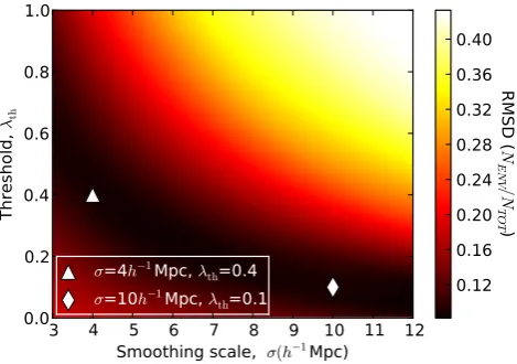
Figure 1. We wish to choose our two free parameters, the eigenvalue thresh-old,λth, and the smoothing scale,σ, in a way that optimizes the resulting statistics by assigning a comparable number of objects to each geometric environment. This plot displays the RMSD (as defined by equation 6), in the number of galaxies in our sample which are assigned to each geometric environment as a function ofλthandσused to generate the classifications. The dark curve represents the statistically optimal region in the parameter space, motivating our choice of two parameter sets: (σ,λth)=(4h−1Mpc, 0.4) and (10h−1Mpc, 0.1), as indicated in the figure.
of the resulting web with the distribution of matter, but such sub-jectivity is undesirable. Instead, in this work we choose to set the value of the eigenvalue threshold in order to optimize the statistical significance of any measurement that we might choose to make in the different environments, i.e. to allocate the objects under study to the four environments as equally as possible. To do so, for a vari-ety of parameter sets we calculate the root mean square dispersion (RMSD) of the fraction of all galaxies in the selected sample (see Section 3.1) classified as each of the four geometric environments from the mean fraction. That is, we calculate the RMSD, defined as
RMSD(Xi)=
3
0(Xi−0.25)2
4 Xi=
NENV,i
NTOT
, (6)
whereNENV,iis the number of galaxies belonging to environmenti,
andNTOTis the total number of galaxies in the full sample, so that
environmentiholds a fractionXiof all galaxies. Fig.1shows this
RMSD in environmental number count as a function of the smooth-ing scale,σ, and the imposed eigenvalue threshold,λth. We wish to
minimize this quantity in order to ensure that all environments hold enough galaxies to maintain a low level of statistical uncertainty, which is essential in order to look for potentially small modulations due to geometric environments. No choice of parameters produces an exactly equal split, where each environment holds 25 per cent of galaxies, but there exists a range of parameters such that each environment holds at least 10 per cent. The dark shaded region rep-resents this optimal parameter space – for smaller smoothing scales we require a higher threshold in order to maintain a near-comparable split of galaxies and vice versa. Based on this, we focus on envi-ronments defined by the parameter sets shown by the symbols in the figure: (σ,λth)=(4h−1Mpc, 0.4) and (10h−1Mpc, 0.1). The
resulting partition of galaxies and of the survey volume between the environments defined by these two parameter sets are given in Table1. We note that these parameters do in fact produce envi-ronments that seem visually plausible, even though this was not a criterion.
3 A P P L I C AT I O N T O G A M A
3.1 GAMA
[image:4.595.46.281.56.221.2] [image:4.595.72.523.618.731.2]We use data from the GAMA survey (Driver et al.2009, 2011; Liske et al. submitted), a spectroscopic redshift survey split be-tween five regions. GAMA is an intermediate redshift survey, bridg-ing the gap between wide-field surveys such as 2dFRGS (Colless et al.2001) and SDSS (York et al.2000) and high-redshift deep field surveys such as VIPERS (Garilli et al.2014). By surveying a cosmologically representative volume whilst maintaining an im-pressive>98 per cent redshift completeness in the equatorial fields (Robotham et al.2010), GAMA provides an ideal data set with which to study the modulation of galactic properties by large-scale environments. In full, GAMA observes galaxies out to z 0.5 andr<19.8; but in this work we study the lower redshift regime where the number density and magnitude range of observed galaxies is statistically sufficient. For consistency with the previous analy-sis of the environmental dependence of the LF within GAMA by (McNaught-Roberts et al.2014, hereafterMNR14), we use a sam-ple of 113 000 galaxies satisfying 0.04< z <0.263 selected from the three equatorial regions of GAMA: G09, G12 and G15, each spanning 12◦×5◦. When testing the effects of the chosen sample, we found no benefit to restricting the catalogue to a volume-limited subset, hence no absolute magnitude cuts are imposed. We use all galaxies with a GAMA redshift quality rating ofnQ>2, indicating
Table 1. Best-fitting parameters found for a non-linear least squares Schechter function (equation 8) fit to the conditional LF of each environment, classified with either (σ, λ)=(4h−1Mpc,0.4) or (10h−1Mpc,0.1).αshows no clear trend with environment,φ∗shows a significant, steady increase from voids to knots andM∗brightens from voids to knots. Errors are calculated from the standard deviation of the resultant parameters for nine jackknife realizations. Note that we expect there to be some degeneracy betweenαandM∗. The sixth and seventh columns show the percentage of the volume and the percentage of galaxies within our sample classified as each environment, respectively. The final column gives the average local overdensity, ¯δ8env, of galaxies in each environment, plotted as the dashed vertical lines in the overdensity histograms of Fig.4.
Environment σ(h−1Mpc) α log10[φ∗/ h−3Mpc−3] M∗−5 logh fenv(per cent) Galaxies (per cent) δenv8¯
Voids 4 −1.25±0.02 −2.38±0.02 −20.54±0.03 59 18 −0.16
Sheets 4 −1.23±0.02 −1.90±0.04 −20.83±0.04 29 34 0.81
Filaments 4 −1.22±0.02 −1.51±0.04 −21.01±0.05 10 36 2.38
Knots 4 −1.27±0.06 −1.19±0.14 −21.22±0.14 1 12 4.39
Voids 10 −1.29±0.03 −2.39±0.06 −20.69±0.06 37 15 −0.03
Sheets 10 −1.22±0.02 −2.05±0.03 −20.78±0.03 39 32 0.69
Filaments 10 −1.24±0.02 −1.75±0.03 −20.99±0.04 20 39 1.93
Knots 10 −1.25±0.04 −1.40±0.09 −21.07±0.09 3 15 3.82
at University of St Andrews on April 24, 2015
http://mnras.oxfordjournals.org/
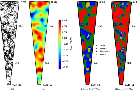
Figure 2. An example of the classification of geometric environments within the GAMA G12 field. (a) Distribution of galaxies within±1◦of the central declination. (b) The density contrast field,δ, derived from (a) after interpolation of the galaxies on to a Cartesian mesh and smoothing with a Gaussian kernel of effective widthσ=10h−1Mpc, with a colour scale proportional to log10(δ+1) as given by the colour bar to the right. (c) The resulting geometric environment classifications, with an eigenvalue threshold ofλth=0.1, from the smoothed density contrast field in (b). (d) The geometric environments for the second parameter set, (σ, λth)=(4h−1Mpc,0.4). Environments are colour coded as shown in the key, e.g.: red, green, blue and yellow for voids, sheets, filaments and knots, respectively. Whilst panel (a) shows a 2D projection of galaxies, the slices shown in panels (b), (c) and (d) show the 2D plane of the central declination; they show the value (density contrast or environment) of whichever cell is intersected by the central declination.
the redshift is sufficiently reliable to be included in scientific analy-ses, and an appropriate visual classification flag (VIS CLASS=0,1 or 255; Baldry et al.2010).
3.2 Observed cosmic web within GAMA
We construct a density field from the GAMA galaxies detailed above for each of the three equatorial fields separately. As discussed in Section 2.1, and in more detail in Appendix A, the volume imme-diately outside the survey region is populated with cloned galaxies reflected along the boundaries of each field. This is in order to re-duce the effects of the survey geometry when smoothing the density field.
Fig.2illustrates the main steps in the classification of one of the GAMA fields. The galaxies are interpolated on to a Cartesian grid and an overdensity field generated by comparison with the catalogue of randomly positioned cloned galaxies. This overdensity field is smoothed by a Gaussian window function of widthσsin Fourier
space. Following that, the potential and its second derivatives are calculated, from which the 3 eigenvalues can be derived for each cell of the grid. We approximate the dimensionality of collapse by the number of eigenvalues above the chosen eigenvalue threshold and from this each cell is classified as either a void, sheet, filament
or knot. Finally, the galaxy catalogue is split into four environmen-tally defined subcatalogues by assigning the galaxies the geometric environment of the cell in which they reside.
In Fig.2(a), we plot the distribution of all galaxies within±1◦ of the central declination of the G12 field. Fig.2(b) is the resulting density field along the central declination of the G12 field, after smoothing with an effective smoothing scale ofσ =10h−1Mpc.
In Fig.2(c) and Fig.2(d), we show the resulting geometric environ-ments of the central declination slice of the G12 field for our two parameter sets, (σ, λth)=(10h−1Mpc,0.1) and (4h−1Mpc,0.4),
respectively. As may be expected, both figures display a similar basic skeleton, with the larger smoothing scale resulting in larger geometric structures. The knots in particular are visibly larger in Fig.2(c).
3.3 Geometric environments of GAMA galaxies
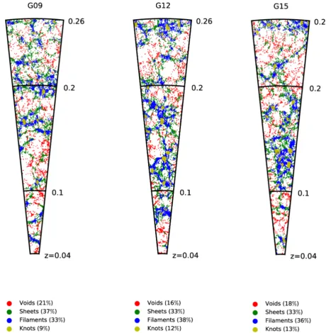
The geometric environments of all galaxies in the sample are defined by the classification of the cell they belong to. In Fig.3, we plot the geometric environment classifications of galaxies around the central declination slice of each of the 3 GAMA fields. We show here envi-ronments defined for the parameter set (σ, λth)=(4h−1Mpc,0.4).
Although the sheets are not visually well captured in a 2D figure, the galaxies in filaments stand out clearly, particularly when the
at University of St Andrews on April 24, 2015
http://mnras.oxfordjournals.org/
Figure 3. The distribution of galaxies in the three equatorial GAMA fields within±1◦of the central declination. Galaxies are colour coded by their resulting geometric environment classification after smoothing with a Gaussian of widthσ =4h−1Mpc and applying a threshold ofλ
th=0.4. For each of the GAMA fields, the percentage of galaxies within each of the four environments is shown in the keys beneath the cones.
filament happens to lie in the plane of the figure.1The void
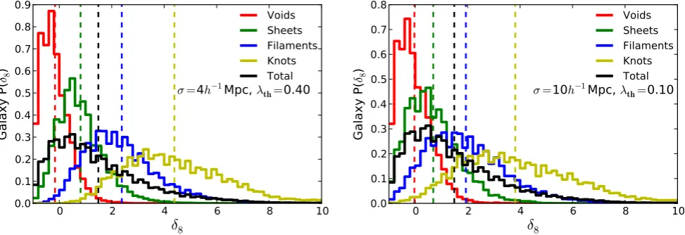
galax-ies are in less populated regions but sometimes exhibit small-scale clustering which has been smoothed out during the filtering process. As well as having a distinct shape, the different geometric envi-ronments are also strongly distinct in terms of density. The distri-butions of local overdensities within each geometric environment are shown in Fig.4, where the overdensity is calculated from the number of galaxies within a sphere of radius 8h−1Mpc centred
on the location of each galaxy rather than the grid-based overden-sity measure used during the environment classification process.
1For an animated view of the 3D distribution of geometric environments, seehttp://www.roe.ac.uk/ee/GAMA
This density measure follows from the work of Croton et al. (2005) and is chosen for consistency withMNR14; it involves selecting a density-defining population of galaxies which form a volume-limited sample over our redshift range. All galaxies within the 8h−1Mpc radius contribute to the density measure if they are part
of the density-defining population, including the galaxy for which we are measuring the density. We convert the measured densities toδ8, our measure of overdensity, by comparison with the effective
mean density within the sample.
As expected, the average overdensity increases as the dimen-sionality of the environment decreases (note that the 3D voids are the highest dimension of environment, with knots considered to have the lowest dimensionality, having collapsed in all dimensions); most void galaxies are found in underdense regions, almost no knot
at University of St Andrews on April 24, 2015
http://mnras.oxfordjournals.org/
Figure 4. Distribution of local overdensities for galaxies split by geometric environment. Dashed lines indicate the average overdensities, as given in Table1, of all galaxies within each environment. The overdensity,δ8, is derived from the number of galaxies within a sphere of radius 8h−1Mpc. The overdensity increases as the dimension of the environment reduces; but because there is a wide range of overdensities in each environment we can look for a dependence of galaxy properties onδ8and geometric environment separately.
galaxies reside in underdense regions and instead live in highly overdense areas. One may be surprised that a significant proportion of voids are found to be slightly overdense; a similar result was found in the analysis of simulated data by Alonso et al.2015. If we retain the simplicity of an environment classification using the tidal tensor, this feature cannot be entirely removed. The fraction of overdense voids is reduced if the threshold,λth, is made smaller, but
extreme low thresholds do not produce a good visual impression of the web and result in apparently 3D regions being classified as a 2D sheet. The broad distribution of densities within each envi-ronment shows the geometric envienvi-ronment holds more information than the density alone. Environments derived from the 10h−1Mpc
smoothed density field show a slightly larger spread of densities in any given environment than for the 4h−1Mpc field, though the
distributions are relatively similar.
An alternative method of classifying LSS within GAMA using minimal spanning trees was presented in Alpaslan et al. (2014). In Appendix C, we compare our results, finding a strong visual agreement for the filamentary regions but limited agreement in our classification of voids. With the somewhat flexible definitions of geometric environments this is neither a surprise nor cause for concern. On the contrary, it illustrates the variety of meanings of terms such as voids, even within the context of the cosmic web. Hence, when interpreting any results in the context of the web, it is important for one to have a clear quantitative understanding of the how the environments in question are defined.
4 L F s A N D G E O M E T R I C E N V I R O N M E N T
The galaxy LF is measured independently for each geometric en-vironment, usingk-corrected and luminosity evolution corrected absoluter-band magnitudes,Mer, and following the approach taken inMNR14. This method adopts the step-wise maximum likelihood estimator (Efstathiou, Ellis & Peterson1988), and normalizes the LF taking into account the effective fraction of the volume covered by a given geometric environment (fenv, estimated by counting the
number of galaxies in the unclustered random catalogue that fall within the regions classified as each environment):
Nenv=fenvtot
z2
z1
dz dV dzd
Mbright(z)
Mfaint(z)
φ(M) dM (7)
for a galaxy sample with Nenv galaxies in a given environment,
redshift limitsz1andz2and total solid angletot.
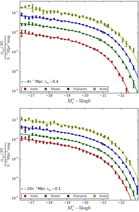
The resultant conditional LFs for each geometric environment are shown in Fig.5with jackknife error bars. These conditional LFs reveal a higher number density of luminous galaxies in lower dimensional environments, introducing a vertical shift of the LF. We use a Schechter function (Schechter1976),
φ(M)= ln 10 2.5 φ
∗100.4(M∗−M)(1+α)exp (−100.4(M∗−M)), (8)
to characterize the magnitude and shape of the LF. Here,αdescribes the power-law slope of the faint end,M∗describes the magnitude at which there is a break from the power law, or the ‘knee’ of the LF, andφ∗describes the normalization. The solid lines of Fig.5
show fitting Schechter functions for each LF, with the best-fitting parameters given in Table1. There is a clear increase in the normalization of the LF from voids to knots, shown by the steady increase ofφ∗. The turnover point,M∗, of the LFs moves towards brighter magnitudes from voids to knots, suggesting that brighter galaxies have an increased bias towards lower dimensional regions. Note that we expect there to be some environmentally dependent degeneracies in theαandM∗parameters (see fig. D1 ofMNR14).
A comparison of the upper and lower panels in Fig.5shows the impact of the choice of different smoothing scales and thresholds. Using a range of parameters following the optimal black curve in Fig.1, it was found that the magnitude of the difference between the conditional LFs increases as the smoothing scale decreases or as the eigenvalue threshold decreases. This tends to introduce only a vertical shift to the functions, characterized byφ∗, whilst the shapes of the LFs do not show significant dependence on the smoothing and threshold parameters. The variation in shape between the LFs of each geometric environment are discussed further in the following section.
4.1 Reference Schechter functions
In order to remove some of the vertical offset and clarify the differ-ence in shape between the LFs of each geometric environment, in Fig.6we plot the ratio of the conditional LFs to a set of scaled refer-ence Schechter functions. The referrefer-ence function,φref, tot, is found
by fitting a Schechter function to all galaxies in the sample. We
at University of St Andrews on April 24, 2015
http://mnras.oxfordjournals.org/
Figure 5. The galaxy LFs and corresponding jackknife errors of the four subcatalogues produced by splitting the GAMA sample according to geo-metric environment, defined withσ =4 or 10h−1Mpc. Solid lines show best-fitting Schechter functions for each conditional LF, open circles show with the best-fitting value ofM∗, given in Table1. The normalization, orφ∗ in a Schechter function fit, is seen to increase significantly between high-and low-dimensional environments.
apply a normalization for each environment to produce the scaled reference Schechter functions,φref, env, given by
φref,env= (1+
¯
δenv 8 )
(1+¯δtot 8 )
×φref,tot, (9)
where ¯δenv
8 is the average overdensity within an 8h−1Mpc sphere
centred on each galaxy of the environment and ¯δtot
8 is that of all
the galaxies in the full sample (we find ¯δtot
8 =8×10⁻³). The solid
lines in Fig.6show the ratio of the best-fitting Schechter functions for each environment to the reference functions, data points show the ratio for the measured LFs. The departure from the global shape is seen to increase towards the bright end of the LF; the number density of void galaxies decreases as we move towards brighter magnitude bins faster than that of the global population whereas we see a slower decline with brightness for the knot galaxies. The remaining vertical offset is likely to be due to the approximations used in definingφref, env: for example, we do not consider the effect
[image:8.595.48.279.56.407.2]of bias, i.e. galaxies are biased tracers of the underlying dark matter density field and the degree of bias may vary between environments.
Figure 6. Observed environmental LFs (points) and their best-fitting Schechter functions (solid) divided by the scaled reference Schechter func-tions of equation (9) for each geometric environment, colour coded as shown in the legend. The difference in the shape of the LF between the environ-ments is most apparent at the bright end of the LF, owing to the decrease of the turnover magnitude,M∗, from voids to knots. Note that the linear scaling means that, for example, a factor of 2 in excess is more noticeable than a factor of 2 in deficit.
4.2 Direct dependence on geometric environment
It is clear from the results ofMNR14and others (e.g. H¨utsi et al.
2002; Croton et al.2005; Tempel et al.2011) that local density plays a significant role in determining the number density of lu-minous galaxies. In this section, we ask whether the geometric environment plays anyadditionalrole. Is it correct to assume that the LF, given a certain local overdensity, will be the same regardless of location within the cosmic web? The analytic results of the de-pendence of the Schechter fit parameters on local density,φ(M|δ8),
presented inMNR14could be used to answer this question; how-ever, we found statistical uncertainties in the fit parameters at the extremes ofδ8limited its use. Instead, we sample the galaxies in
such a way as to remove any additional geometric information from the environment-split subcatalogues, whilst retaining the distribu-tion of local densities. We recalculate the LFs for these resam-pled catalogues with the hypothesis that any direct modulation by
at University of St Andrews on April 24, 2015
http://mnras.oxfordjournals.org/
Figure 7. The proportion of galaxies from each true geometric environment which were sampled to make up the new shuffled-galaxy catalogues. Shuf-fled catalogues are predominantly composed of galaxies which were also in the original environment catalogue, as is expected from the distribution of overdensities shown in Fig.4. However, there is still significant mixing between environments due to the overlap of the histograms seen in Fig.4, which should change the resultant LF if the geometric environment is having a direct influence.
geometric environment will present itself as a disparity between these results.
We populate four ‘shuffled’ catalogues by randomly selecting GAMA galaxies from within overdensity bins, such that theδ8
dis-tribution of each shuffled catalogue matches that of one of the orig-inal geometric-environment-split catalogues. This can be thought of as shuffling the galaxies around within regions of the same over-density (bins of width 0.1 inδ8are used). For each galaxy that was
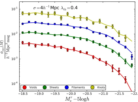
included in the original LF, we pick at a random a galaxy with the same local overdensity and effectively replace the original galaxy with this new one. Thus the overall effect is to remove the geometric environment distinction contained in the original catalogues, whilst maintaining the same distribution of local densities.
A volume-limited sample is required to allow galaxies to be shuffled randomly over different redshifts without moving galaxies out of their observable redshift range. We use a sample of26 000 galaxies satisfying 0.021< z <0.137 and−22< Mre−5 logh <
−18.5, chosen as a compromise between a large magnitude range and a large sample size. In Fig.7, we show the proportion of galaxies in each shuffled catalogue which were taken from each of the four ‘true’ geometric environments defined with our smaller smoothing scale parameter set, (σ, λth)=(4h−1Mpc,0.4). For example, the
bottom panel of Fig.7shows that50 per cent of the galaxies in the shuffled-knots catalogue are from a filament environment, and the remaining40 and10 per cent of galaxies were drawn from knot and sheet environments, respectively. The combined distribution of densities of this selection of galaxies making up the shuffled-knots catalogue matches the distribution seen in the original shuffled-knots catalogue. A large fraction of the galaxies in each shuffled catalogue were also in the original geometric environment catalogue, as is expected from the distribution of overdensities, but there is still significant mixing due to the overlap of the histograms seen in Fig.4. When repeating the shuffling for theσ=10h−1Mpc geometric
environments, we see more mixing between environments due to the slighter broader distribution of densities in any given environment, with more than half the galaxies of each shuffled catalogue being selected from a different geometric environment. We argue that, if geometric environment has a significant direct effect, we should see different LFs for each shuffled catalogue, in which geometric information is lost, as compared with the initial geometrically split catalogue.
[image:9.595.52.278.59.160.2]Fig.8shows the LF for each environment, given by the circles and jackknife error bars, and for an average over nine realizations
Figure 8. The conditional galaxy LFs of the volume-limited sample de-scribed in Section 4.2. The LFs for the true geometric environments are indicated by the circle markers, with jackknife error bars. For each geomet-ric environment, we create nine realizations of a shuffled catalogue which mimics the distribution of overdensities in the geometric environment but selects galaxies randomly regardless of local geometry. The solid lines plot the average of the nine realizations for each environment and can be seen to be fully consistent with the original LFs, indicating the galaxy LF is independent of geometry for a given overdensity.
Figure 9. The volume-limited LF and jackknife errors for each geometric environment, divided by the average LF of nine realizations of shuffled catalogues composed of galaxies selected randomly from the full volume to mimic the density distribution of the corresponding geometric environment. Dashed lines represent a ratio of 1, indicating no variation between the geometric and the shuffled LFs. No statistically significant deviation away from a ratio of 1 is seen, which leads us to conclude the shuffled catalogues are consistent with the original LF and the cosmic web has no detectable direct influence.
of shuffled catalogues, shown by the solid lines. The LFs of the original and the shuffled catalogues are fully consistent, indicat-ing that the local overdensity is the only significant environmental property affecting the galaxy LF and the cosmic web has no direct influence. The ratio between the geometric- and the shuffled-LFs, shown in Fig.9, further emphasises that we find no statistically sig-nificant difference between the two measurements. We show only the (σ, λth)=(4h−1Mpc,0.4) results here, noting that the same
analysis applied to the geometric environments as classified with (σ, λth)=(10h−1Mpc,0.1) draws the same conclusion.
at University of St Andrews on April 24, 2015
http://mnras.oxfordjournals.org/
[image:9.595.311.545.337.513.2]We tested the scale dependence of this result by repeating the shuffling process with densities defined over spheres of radii 6 and 12h−1Mpc, finding no significant differences in our results. As a
further test, we shuffled the geometric classifications of individual cells of the initial Cartesian grid within density bins where the density was defined by the smoothed density field (4 or 10h−1Mpc)
used to initially generate the geometric classifications. This has the advantage that we do not require a volume-limited sample and hence can test the full magnitude range. Again we found no statistically significant difference, reinforcing the main result of this paper, that the galaxy LF is independent of geometry for a given smoothed density. We also note that, on testing a range of thresholds within the dark curve of Fig.1, we found no change in the overall conclusions of this paper.
5 S U M M A RY A N D D I S C U S S I O N
In this paper, we have developed a method for probing the cos-mic web in galaxy redshift surveys, which has been applied to the GAMA data set. Of the many tools that have been proposed for picking out the skeleton of LSS, we have rejected those that depend on unobservable velocity information, and focused on a simple technique based on the tidal tensor – the Hessian matrix of second derivatives of the pseudo-potential that is sourced by the galaxy density fluctuation. This allows the survey volume to be dissected into its four distinct geometrical environments – voids, sheets, fila-ments and knots – based on the number of eigenvalues of the tidal tensor that lie above a threshold.
We have explored different choices for the threshold and iden-tified a practical option in which galaxies are distributed roughly equally between different components of the web, allowing good statistics in the comparison of properties as a function of environ-ment. We have carried out tests with simulations to show how this method can yield robust environmental classifications in the pres-ence of real-world effects such as redshift-space distortions, bias and survey geometry. In particular, we applied a method where the data are reflected at the survey boundaries in order to mitigate a bias that would otherwise arise if the survey was simply zero-padded. This has allowed us to search for the impact of large-scale tidal forces on the galaxy population, and there have been a number of studies suggesting that an effect of this sort should be present.
Metuki et al. (2015) conducted a thorough analysis of galaxy properties within the cosmic web, finding significant dependences on location, which they attributed largely to the strong relationship between galaxy properties and the properties of their host haloes, which are in turn linked to their geometric environments. They found that the strong dependence of the halo mass function on the cosmic web was the main cause of the apparent dependence of galaxy properties. However, these analyses often do not test whether the relationships found can be directly attributed to a modulation by geometric environment, or rather are manifestations of the indirect influence of the local-density field. In fact, Alonso et al. (2015) show that, based on Gaussian statistics within the linear regime, we expect a variation of the halo mass function within different web components that is due solely to the underlying density field; there is no coupling to tidal forces and the theoretical halo mass function is independent of geometry at a given local density.
Yan, Fan & White (2013) studied the tidal dependence of galaxy properties using the ellipticity, constructed from the eigenvalues of the tidal tensor in a way that exhibits lessδ-dependence as a mea-sure of environment than the classification method used in this work. Their analysis of SDSS data revealed no physical influence of
en-vironmental morphology on galaxy properties. Similarly, Alpaslan et al. (in preparation) investigated the relations between various galaxy properties and LSS identified within the GAMA data set by the methods discussed in Appendix C. They found the environment had limited direct impact on galaxy properties, with the stellar mass of a galaxy playing a far larger role in shaping its evolution than the galaxy’s location within the cosmic web. However, when iden-tifying filaments by the ‘Bisous’ process, Guo et al. (2014) find a disparity between the LFs of satellite galaxies in SDSS whose host galaxy resides in a filament and those whose host galaxy does not, which they claim cannot be attributed to an environmental bias. Re-cent work has found a direct relationship between LSS anistropies and the cosmic web when considering tensor properties such as the spin of galaxies (Libeskind et al.2012) and angular momentum of dark matter substructures (Dubois et al.2014). These authors find a correlation between the orientation of LSS and the axes of the cosmic web.
With this context, the main results of the GAMA-based analysis in this paper can be summarized as follows.
(i) We have measured the galaxy LF in each component of the web and found a strong variation. By fitting a Schechter function to each conditional LF we quantify the variation of the LF between web components. The normalization, described byφ∗, increases by a factor of∼10 from voids to knots. The knee of the LF,M∗, brightens from voids to knots by 0.7 and 0.4 mag for 4 and 10h−1Mpc
smoothing scales, respectively. We find no clear trend inα, the parameter describing the faint end slope of the LF.
(ii) We test the direct influence of the cosmic web by investigating the extent to which the observed modulation may be attributed to variations in the local density. For each object, we measure the local overdensity over a range of scales, 6< r <12h−1Mpc, by
counting neighbouring objects within a sphere of radiusr. We find, in all cases, that the modulation may be entirely accounted for by the variations in density between the geometric environments, indicating that the galaxy LF is independent of geometry at a given local density.
Our results are thus consistent with a picture in which scalar properties of halo and galaxy populations have nodirect depen-dence on their location within the geometry of the cosmic web. Our clearly detected variation in the LF of galaxies between differ-ent geometrical environmdiffer-ents can be differ-entirely accounted for via the known correlation of galaxy properties with local overdensity, plus the tendency for different locations in the web to sample different densities. It would however be premature to argue on this basis that tidal effects have no impact on the assembly of galaxy structures. It is possible that such higher-order influences are simply too small to be detected at the resolution of this analysis. The scales that we have chosen to probe are set by the requirement of classifying the entire volume of a survey in a way that is robust given the limited number density of galaxies. Higher density regions could be studied to higher spatial resolution, and it may be that some of the published claims of detected tidal effects might yet be validated. But it is clear from the current study that such effects are highly subdominant.
Whilst this paper considers only the galaxy LF, there are a num-ber of other observable properties that would benefit from a thor-ough analysis of the direct influence of the cosmic web. Galaxy colour, mass, morphology and star formation history may all ex-hibit some environmental dependences. Additionally, there may be reason to expect satellite, or low-mass galaxies to be more strongly linked to their geometrical environment (e.g. Carollo et al.2013). Finally, it remains to be seen whether claims of anisotropy within
at University of St Andrews on April 24, 2015
http://mnras.oxfordjournals.org/
different geometrical environments are intrinsic or whether they can be fully accounted for by secondary correlations with overdensity, as explored here for the LF. We can therefore envisage considerable future applications of the tools we have established for the practical exploration of the cosmic web in real galaxy surveys.
AC K N OW L E D G E M E N T S
EE acknowledges support from the Science and Technology Facilities Council. TMR acknowledges support from a ERC Start-ing Grant (DEGAS-259586). CH acknowledges support from the ERC under the EC FP7 grant number 240185. PN acknowledges the support of the Royal Society through the award of a University Research Fellowship and the ERC, through receipt of a Starting Grant (DEGAS- 259586). Data used in this paper will be available through the GAMA DB (http://www.gama-survey.org/) once the as-sociated redshifts are publicly released. GAMA is a joint European-Australian project based around a spectroscopic campaign using the Anglo-Australian Telescope. The GAMA input catalogue is based on data taken from the Sloan Digital Sky Survey and the United Kingdom Infrared Telescope Infrared Deep Sky Survey. Comple-mentary imaging of the GAMA regions is being obtained by a number of independent survey programmes including GALEX MIS, VST KIDS, VISTA VIKING, WISE, Herschel-ATLAS, GMRT and ASKAP providing UV to radio coverage. GAMA is funded by the STFC (UK), the ARC (Australia), the AAO, and the participating institutions. The GAMA website ishttp://www.gama-survey.org/.
The MultiDark Database used in this paper and the web ap-plication providing online access to it were constructed as part of the activities of the German Astrophysical Virtual Observatory as result of a collaboration between the Leibniz-Institute for As-trophysics Potsdam (AIP) and the Spanish MultiDark Consolider Project CSD2009-00064. The Bolshoi and MultiDark simulations were run on the NASA’s Pleiades supercomputer at the NASA Ames Research Center. The MultiDark-Planck (MDPL) and the BigMD simulation suite have been performed in the Supermuc supercom-puter at LRZ using time granted by PRACE.
R E F E R E N C E S
Alonso D., Eardley E., Peacock J., 2015, MNRAS, 447, 2683 Alpaslan M. et al., 2014, MNRAS, 438, 177 (A14)
Arag´on-Calvo M. A., van de Weygaert R., Jones B. J. T., 2010, MNRAS, 408, 2163
Baldry I. K. et al., 2010, MNRAS, 404, 86
Balogh M. L., Baldry I. K., Nichol R., Miller C., Bower R., Glazebrook K., 2004, ApJ, 615, L101
Bardeen J. M., Bond J. R., Kaiser N., Szalay A. S., 1986, ApJ, 304, 15 Barrow J. D., Bhavsar S. P., Sonoda D. H., 1985, MNRAS, 216, 17 Brough S. et al., 2013, MNRAS, 435, 2903
Carollo C. M. et al., 2013, ApJ, 776, 71
Cautun M., van de Weygaert R., Jones B. J. T., 2013, MNRAS, 429, 1286 Codis S., Pichon C., Devriendt J., Slyz A., Pogosyan D., Dubois Y., Sousbie
T., 2012, MNRAS, 427, 3320 Cole S., 2011, MNRAS, 416, 739
Cole S., Kaiser N., 1989, MNRAS, 237, 1127 Colless M. et al., 2001, MNRAS, 328, 1039 Croton D. J. et al., 2005, MNRAS, 356, 1155 de la Torre S. et al., 2013, A&A, 557, A54 Dressler A., 1980, ApJ, 236, 351
Driver S. P. et al., 2009, Astron. Geophys., 50, 12 Driver S. P. et al., 2011, MNRAS, 413, 971 Dubois Y. et al., 2014, MNRAS, 444, 1453
Efstathiou G., Ellis R. S., Peterson B. A., 1988, MNRAS, 232, 431
Falck B. L., Neyrinck M. C., Szalay A. S., 2012, ApJ, 754, 126
Forero-Romero J. E., Hoffman Y., Gottl¨ober S., Klypin A., Yepes G., 2009, MNRAS, 396, 1815
Forero-Romero J. E., Contreras S., Padilla N., 2014, MNRAS, 443, 1090 Garilli B. et al., 2014, A&A, 562, A23
G´omez P. L. et al., 2003, ApJ, 584, 210
Guo Q., Tempel E., Libeskind N. I., 2014, preprint (arXiv:1403.5563) Hahn O., Porciani C., Carollo C. M., Dekel A., 2007, MNRAS, 375, 489 Hahn O., Porciani C., Dekel A., Carollo C. M., 2009, MNRAS, 398, 1742 Hoffman Y., Metuki O., Yepes G., Gottl¨ober S., Forero-Romero J. E.,
Libe-skind N. I., Knebe A., 2012, MNRAS, 425, 2049
H¨utsi G., Einasto J., Tucker D. L., Saar E., Einasto M., M¨uller V., Hein¨am¨aki P., Allam S. S., 2002, preprint (astro-ph/0212327)
Kauffmann G., White S. D. M., Guiderdoni B., 1993, MNRAS, 264, 201 Libeskind N. I., Hoffman Y., Knebe A., Steinmetz M., Gottl¨ober S., Metuki
O., Yepes G., 2012, MNRAS, 421, L137 Ludlow A. D., Porciani C., 2011, MNRAS, 413, 1961
McNaught-Roberts T. et al., 2014, MNRAS, 445, 2125, (MNR14) Metuki O., Libeskind N. I., Hoffman Y., Crain R. A., Theuns T., 2015,
MNRAS, 446, 1458
Moster B. P., Somerville R. S., Maulbetsch C., van den Bosch F. C., Macci`o A. V., Naab T., Oser L., 2010, ApJ, 710, 903
Platen E., van de Weygaert R., Jones B. J. T., 2007, MNRAS, 380, 551 Prada F., Klypin A. A., Cuesta A. J., Betancort-Rijo J. E., Primack J., 2012,
MNRAS, 423, 3018
Robotham A. et al., 2010, PASA, 27, 76
Robotham A. S. G. et al., 2013, MNRAS, 431, 167 Schechter P., 1976, ApJ, 203, 297
Sheth R. K., Mo H. J., Tormen G., 2001, MNRAS, 323, 1 Sousbie T., 2011, MNRAS, 414, 350
Tempel E., Saar E., Liivam¨agi L. J., Tamm A., Einasto J., Einasto M., M¨uller V., 2011, A&A, 529, A53
Vale A., Ostriker J. P., 2004, MNRAS, 353, 189 van den Bosch F. C. et al., 2007, MNRAS, 376, 841 Wijesinghe D. B. et al., 2012, MNRAS, 423, 3679 Yan H., Fan Z., White S. D. M., 2013, MNRAS, 430, 3432 York D. G. et al., 2000, AJ, 120, 1579
Zel’dovich Y. B., 1970, A&A, 5, 84
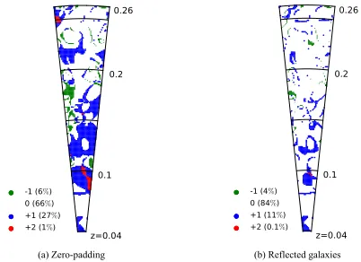
A P P E N D I X A : E F F E C T S O F T H E S U RV E Y G E O M E T RY
A significant limitation of the tidal tensor prescription, or of any analysis requiring information on the smoothed density field, is that observational data sets lack information beyond the surveyed region. There is then the question of how to smooth the galaxy distribution near the survey boundaries. If one ‘zero-pads’ the volume outside of the survey, by setting it all to the large-scale average overdensity (¯δ=0 by definition) this will, on average, reduce the magnitude of both overdensities and underdensities that may be straddling the border of the survey and alter our estimate of the true underlying density in a systematic but unpredictable way. To mitigate this effect, we ‘reflect’ the galaxies along each field’s boundaries in right ascension (RA) and declination (Dec.). We clone the galaxies inside the survey volume and give them an appropriate reflected location outside of the survey volume before the smoothing process. In effect, we make the reasonable assumption that large-scale features continue smoothly beyond the survey edge.
A sketch illustrating the reflection process is shown in Fig.A1. Each galaxy is cloned three times always keeping its original red-shift, the first clone is given a new RA equivalent to a reflection along the nearest RA border of the field, the second clone keeps the RA of the original galaxy but has its Dec. changed to simulate a reflection along the nearest Dec. boundary of the field, and the third takes on both of these two new RA and Dec. values. This has
at University of St Andrews on April 24, 2015
http://mnras.oxfordjournals.org/
Figure A1. A sketch of the reflection method. Each galaxy in the survey sample, represented by the blue spiral, is cloned three times as depicted by the black spirals. The solid line box represents the RA and Dec. boundaries of the GAMA field, with redshift pointing out of the page. The dotted lines show the quadrant which is reflected along the nearest two boundaries of the field, which are of constant RA or Dec. and shown by the dashed lines. Each long arrow in the figure represents the same difference in RA, similarly each short arrow represents the same difference in declination.
an approximately equivalent effect to using a weighted smoothing kernel, where cells near the edge of the volume are up-weighted to account for the lack of information in cells outside of the volume. However, the reflection approach permits the smoothing operation to be a single convolution, giving us the speed advantage of the fast Fourier transform. Beyond the reflection regions (half the width of the survey dimension) we use zero-padding. In the redshift direc-tion, for each field we make use of the full GAMA galaxy catalogue,
0.0< z <0.5, and calculate a density contrast for the full surveyed
volume of each field, though, as described in the text, we select only galaxies satisfying 0.04< z <0.263 for our scientific analyses. We make use of the MultiDark (1h−1Gpc)3 dark matter simulation
(Prada et al.2012), populated with mock galaxies using halo oc-cupation distribution modelling (de la Torre et al.2013), selecting GAMA-representative regions from the full simulation where nec-essary to test this reflection method. The simulated data set we use is a single redshift snapshot of z = 0.1 with galaxies randomly sampled so that the number density of mock galaxies matches the average number density of galaxies in our GAMA sample. Fig.A2
shows, for the simulated data, the regions in which the resulting environments differ from those when information of the full peri-odic cube is used when only the GAMA-sized volume information is kept, and other regions are either zero-padded only, or popu-lated with the cloned galaxies as described above. We show here results for the 10h−1Mpc smoothing, noting that the 4h−1Mpc
smoothing is less affected by the survey geometry (due a reduced ‘skin-depth’ of volume which is significantly affected by the vol-ume outside of the survey), but shows a similar improvement when using this reflection technique. The differences are not confined to the edges of the survey due to the use of Fourier transforms but instead tend to occur along boundaries between regions of different environments due to a slight change in the calculated eigenvalues. The percentages of cells classified differently, measured over three realizations, are given in the key of Fig.A2. It can be seen that the reflection technique is beneficial, increasing the percentage of correctly classified cells from 66 to 84 per cent so that the classifi-cations more closely mimic the results of the full simulation than when zero-padding alone is used. There are remaining unavoid-able discrepancies due to the lack of information, however we note that 99.9 per cent of cells are classified within±1 dimension of
en-Figure A2. A test of the effect of the survey geometry on the resulting geometric environment classifications using simulated data. Coloured re-gions of the figure show the cells which are classified differently to the full simulation results when regions outside a GAMA sized survey cone are zero-padded (left-hand panel) or filled with reflected galaxies (right-hand panel), as described in the text. This is for an example realization of a GAMA field and (σ,λth)=(10h−1Mpc, 0.1). Colour code in the keys refer to the difference,N, in the number of eigenvalues above the threshold,N+, be-tween the full simulation and the limited-information survey classifications, e.g.N=NFULL+ −N0pad+ . Hence each cell has a discrete value ofN, with−3≤N≤3. The percentage of all cells with a givenN, measured over three realizations, is indicated in the keys. We wish to maximize the percentage withN=0, as this indicates the limited information has not changed the resultant environment classification of these cells. The increase inN=0 from 66 to 84 per cent shows that the reflection technique offers a strong improvement over zero-padding alone.
vironment from the ‘full-information’ results when the reflection technique is applied, an increase from the corresponding value for zero-padding of 99 per cent.
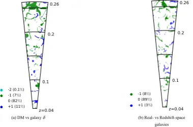
A P P E N D I X B : R E D S H I F T S PAC E
D I S T O RT I O N S A N D OT H E R C O M P L I C AT I O N S
As discussed in Section 2.1, the use of biased galaxies in redshift space to estimate the underlying matter overdensity requires cau-tion. We again make use of the simulated data set to investigate the magnitude of these effects on the resulting environment classifica-tions. The MultiDark simulation provides information on both the underlying dark matter density field and a simulated galaxy cata-logue with galaxy velocity information. This allows us to see how the resulting classifications vary when the density field is estimated from the locations of galaxies and when the underlying dark matter density field is used directly. In a similar manner to Fig.A2, Fig.B1a shows those cells which change their classification when the galaxy density field rather than the dark matter density field is used. The use of galaxies to estimate the density results in 20 per cent of the volume appearing to belong to a different geometric environment.
With the velocity information we are able to shift each galaxy in the simulation to its redshift-space coordinates, by estimating the distance which would have been inferred given its location and radial velocity, and again compute this comparison. Fig.B1b compares the classifications for density fields constructed from redshift- and real-space galaxies. We find the redshift-space dis-tortions to have no effect on 90 per cent of the volume for both 4 and 10h−1Mpc smoothing scales.
We find the combined effect of the three main causes of error when applying the tidal tensor prescription to observational data (survey geometry, a density field sourced from the galaxy number
at University of St Andrews on April 24, 2015
http://mnras.oxfordjournals.org/
[image:12.595.323.524.59.205.2]Figure B1. A test of the effects of redshift-space distortions and of us-ing a density field estimated from galaxy number counts on the resultus-ing geometric environment classifications within simulated data. Coloured re-gions of the figure show the cells which are classified differently, with (σ,λ)=(10h−1Mpc, 0.1), when the dark matter density field is used or the density field is calculated from the (real-space) galaxies (left-hand panel) and when the density field is calculated from the real-space galaxies or from redshift-space galaxies (right-hand panel). Colour code in the keys refer to the difference in the number of eigenvalues above the threshold,
[image:13.595.115.212.334.525.2]N+, between the full simulation and the limited-information survey-style classifications, eg.NDM+ −Ngal+ orNreal+−sp−Nredshift+ −sp. The percentages of cells with each difference value, measured over three realizations, are indicated in the keys.
Figure B2. A test of the effects of limited information in observational cata-logues on resulting geometric environment classifications. Full-information results are computed from the underlying DM density field using the full pe-riodic 1h−1Gpc simulation. Limited-information results use galaxies from the simulation, in redshift space, discarding information outside of a volume representative of a GAMA field and implementing the reflection technique described in the text. Coloured regions of the figure show the cells which are classified differently between the two approaches for an example real-ization of a GAMA field and (σ,λth)=(10h−1Mpc, 0.1). Colour code in the key refers to the difference,N, in the number of eigenvalues above the threshold,N+, between the full simulation and the limited-information survey classifications, e.g.N=NFULL+ −NLIM+ . Hence each cell has a discrete value ofN, with−3≤N≤3. The percentage of all cells with a givenN, within three realizations, is indicated in the key.
density and redshift-space distortions) to be a change in the resulting geometric environment of<25 per cent of the volume for both 4 and 10h−1Mpc smoothing scales. An example realization of a field
is shown in Fig.B2, indicating the regions which are classified
differently when the three causes of error discussed above are all introduced.
A P P E N D I X C : OT H E R G A M A L S S A N A LY S E S
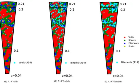
A previous analysis of LSS within the GAMA regions was con-ducted by Alpaslan et al.2014(hereafterA14).A14implemented a minimal spanning tree algorithm to identify 643 filaments within the same three GAMA equatorial regions used in this work, with a slightly lower redshift cut ofz <0.213.A14also identified a secondary population of smaller coherent structures, tendrils, and a population of isolated void galaxies. A comparison of the result-ing environment classifications of galaxies between the two works is presented in Fig.C1; the histograms illustrate, for each A14
population, the number of galaxies belonging to each of our ge-ometric environments. The dashed lines in the figure indicate the number of galaxies in the full GAMA sample in each of our envi-ronments, normalized by the size of the eachA14population, hence the dashed lines indicate the proportion which would be expected from a purely random selection. A visual comparison is presented in Fig.C2, which shows the central declination slice of the G9 field, the geometric environments as classified by this work, and all ob-jects in each of the three populations as identified inA14within
±0.5 deg of the central declination. We find the filaments ofA14to be visually consistent with the filamentary regions identified in this work. The tendrils and voids ofA14favour the underdense environ-ments of voids and sheets. Note that we show here results for our environments computed withσ =4h−1Mpc, a similar scale to the
r=4.13h−1Mpc used inA14as the maximum distance allowed
between a galaxy and a filament. We suggest that the ’void galax-ies’ as identified inA14should be thought of as isolated galaxies, whereas our voids correspond to larger geometric structures.
Figure C1. Comparison between LSS identified inA14and in this work. Each row shows how either the filaments, tendrils or voids identified in A14are classified in this work, withλth=0.4 andσ=4h−1Mpc. The percentages given in the figure show, for eachA14population, the percentage of galaxies in each of the environments in this work. Dashed lines indicate the number of galaxies in the full GAMA sample classified in each of our geometric environments, normalized by the number of galaxies in theA14 population which each row represents. Hence the dashed lines, which are the same for each panel before normalization, can be thought of as the expected distribution of a random selection from all galaxies.
at University of St Andrews on April 24, 2015
http://mnras.oxfordjournals.org/
[image:13.595.328.529.429.626.2]Figure C2. A comparison of LSS identified by this work, and byA14, within the central declination of the G9 field. Our geometric environments, calculated withλth=0.4 andσ =4h−1Mpc, are shown by the background colours with red, green, blue and yellow indicating voids, sheets, filaments and knots, respectively. From left to right, the cyan dots in the figures show the positions of all galaxies within±0.5◦of the central declination in theA14populations voids, tendrils and filaments, respectively.
This paper has been typeset from a TEX/LATEX file prepared by the author.
at University of St Andrews on April 24, 2015
http://mnras.oxfordjournals.org/