R E S E A R C H
Open Access
Numerical approximation to a solution of the
modified regularized long wave equation
using quintic B-splines
Seydi Battal Gazi Karakoc
1, Nuri Murat Yagmurlu
2*and Yusuf Ucar
2*Correspondence:
[email protected] 2Department of Mathematics, Faculty of Science and Art, Inönü University, Malatya, 44280, Turkey Full list of author information is available at the end of the article
Abstract
In this work, a numerical solution of the modified regularized long wave (MRLW) equation is obtained by the method based on collocation of quintic B-splines over the finite elements. A linear stability analysis shows that the numerical scheme based on Von Neumann approximation theory is unconditionally stable. Test problems including the solitary wave motion, the interaction of two and three solitary waves and the Maxwellian initial condition are solved to validate the proposed method by calculating error normsL2andL∞that are found to be marginally accurate and
efficient. The three invariants of the motion have been calculated to determine the conservation properties of the scheme. The obtained results are compared with other earlier results.
MSC: 97N40; 65N30; 65D07; 76B25; 74S05
Keywords: MRLW equation; collocation; finite element method; B-spline; solitary waves
1 Introduction
The modified regularized long wave (MRLW) equation, based upon the regularized long wave (RLW) equation,
Ut+Ux+δUUx–μUxxt= , () which was proposed at first by Peregrine [] to describe the development of an undular bore, has the form
Ut+Ux+ UUx–μUxxt= , () whereδandμare positive parameters and the subscriptsxandtdenote the differentiation. The RLW equation is one of the best known partial differential equations because it de-scribes a large number of important physical phenomena with weak nonlinearity and dis-persion waves such as magneto hydrodynamic and ion-acoustic waves in plasma, phonon packets in non-linear crystals, the transverse waves in shallow water, rotating flow down a tube and pressure waves in liquid-gas bubble mixtures. Bona and Pryant [] have studied the existence and uniqueness of the equation. Benjaminet al.[] have proposed the RLW equation as a numerically superior modification of the Korteweg de-Vries (KdV) equation.
This superiority arises because, unlike the KdV equation, the dispersion relation associ-ated with the linearized RLW equation yields the frequency that is bounded for large wave numbers []. But they have found an analytical solution of the RLW equation under the restricted initial and boundary conditions. So, various numerical techniques have been introduced to solve the equation. These include the finite difference [–], finite element [–], Fourier pseudo-spectral [] methods and the meshfree method []. One of the special properties of the equation is that the solutions may exhibit solitons whose mag-nitudes, shapes and velocities are not changed after the collision. The RLW equation is a special case of the generalized long wave (GRLW) equation having the form
Ut+Ux+δUpUx–μUxxt= , () wherepis a positive integer. Zhang [] has used the finite difference method to solve the GRLW equation for a Cauchy problem. The quasilinearization method based on finite dif-ferences was used by Ramos [] for solving the GRLW equation. Kayaet al.[] have also studied the GRLW equation with the Adomian decomposition method. Roshan [] has solved the GRLW equation numerically by the Petrov-Galerkin method using a linear hat function as the trial function and a quintic B-spline function as the test function. Gardner
et al.[] have developed a collocation solution to the MRLW equation using quintic B-splines finite elements. Khalifaet al.[, ] have obtained the numerical solutions of the MRLW equation using the finite difference method and the cubic B-spline collocation fi-nite element method. Solutions based on the collocation method with quadratic B-spline finite elements and the central finite difference method for time have been investigated by Raslan []. Raslan and Hassan [] have solved the MRLW equation by the colloca-tion finite element method using quadratic, cubic, quartic and quintic B-splines to obtain the numerical solutions of a single solitary wave. Fazal-i-Haqet al.[] have designed a numerical scheme based on the quartic B-spline collocation method for the numerical solution of the MRLW equation. Ali [] has formulated a classical radial basis functions (RBFs) collocation method for solving the MRLW equation. In this paper, we have ob-tained a type of the quintic B-spline collocation procedure in which a nonlinear term in the equation is linearized by using the form introduced by Rubin and Graves [] to solve the MRLW equation. The proposed method is shown to represent accurately the migra-tion of a single solitary wave. Then the interacmigra-tion of two and three solitary waves and the Maxwellian initial condition are studied. The linear stability analysis based on the Von Neumann method is also investigated.
2 Quintic B-spline finite element solution
Let us consider MRLW equation () with the following initial,
U(x, ) =f(x), a≤x≤b, () and boundary conditions:
U(a,t) = , U(b,t) = ,
Ux(a,t) = , Ux(b,t) = ,
Uxx(a,t) = , Uxx(b,t) = , t> .
For the numerical calculation, the solution domain of the problem is restricted over an in-tervala≤x≤b. The interval is partitioned into uniformly-sized finite elements of length
hby the knotsxmsuch thata=x<x<· · ·<xN=b. The set of quintic B-spline functions
{φ–(x),φ–(x), . . . ,φN+(x),φN+(x)}forms a basis over the problem domain [a,b]. We seek the numerical solutionUN(x,t) to the exact solutionU(x,t) in the form of
UN(x,t) = N+
j=–
φj(x)δj(t), ()
whereδj(t) are time dependent parameters to be determined from the boundary and col-location conditions.
Quintic B-splinesφm(x) (m= –()N+ ), at the knotsxmare defined over the interval [a,b] by [].
φm(x) = h ⎧ ⎪ ⎪ ⎪ ⎪ ⎪ ⎪ ⎪ ⎪ ⎪ ⎪ ⎪ ⎪ ⎪ ⎪ ⎪ ⎪ ⎪ ⎪ ⎨ ⎪ ⎪ ⎪ ⎪ ⎪ ⎪ ⎪ ⎪ ⎪ ⎪ ⎪ ⎪ ⎪ ⎪ ⎪ ⎪ ⎪ ⎪ ⎩
(x–xm–), [xm–,xm–], (x–xm–)– (x–xm–), [xm–,xm–], (x–xm–)– (x–xm–)+ (x–xm–), [xm–,xm], (x–xm–)– (x–xm–)+ (x–xm–)
– (x–xm), [xm,xm+], (x–xm–)– (x–xm–)+ (x–xm–)
– (x–xm)+ (x–xm+), [xm+,xm+], (x–xm–)– (x–xm–)+ (x–xm–)
– (x–xm)+ (x–xm+)– (x–xm+), [xm+,xm+], , otherwise.
()
Each quintic B-spline covers six elements so that each element [xm,xm+] is covered by six B-splines. Substituting trial function () into Eq. (), the nodal values ofU,U,Uat the knotsxmare obtained in terms of the element parametersδmby
UN(xm,t) =Um=δm–+ δm–+ δm+ δm++δm+,
Um =
h(–δm–– δm–+ δm++δm+), Um=
h(δm–+ δm–– δm+ δm++δm+),
()
where the symbolsandrepresent first and second differentiation with respect tox, re-spectively. The splinesφm(x) and their four principle derivatives vanish outside the interval [xm–,xm+].
Using a first-order forward difference formula for the time derivative of the U and Crank-Nicolson approximation for the space derivativesUxandUxxin Eq. () leads to
Un+–Un t +
Un+ x +Uxn
+ (UU
x)n++ (UUx)n –μ
Un+ xx –Uxxn
t = . ()
Now, if we apply a linearization technique similar to the one first introduced by Rubin and Graves [] to Eq. (),
UUx
n+
we obtain
Un++t U
n+ x + t
Un+UnUxn+UnUn+Uxn+UnUnUxn+–μUxxn+
=Un–t U
n x– t
UUx
n
–μUxxn + tUnUnUxn.
If we substitute the nodal values ofU,Ux andUxxgiven by () into (), we obtain the following iterative system:
δnm+–( –α+ α–α–α) +δmn+–( – α+ α– α– α)
+δmn+( + α+ α) +δmn++( + α+ α+ α– α)
+δmn++( +α+ α+α–α)
=δmn–( +α+α–α) +δmn–( + α+ α– α) +δmn( + α+ α)
+δmn+( – α+ α– α) +δmn+( –α+α–α), m= ()N, () where
α= t
h ,
α= t
h
δnm–+ δnm–+ δmn+ δnm++δmn+–δmn–– δnm–+ δnm++δmn+,
α= t
h
δnm–+ δnm–+ δmn+ δnm++δmn+,
α= μ
h .
This newly obtained iterative system () consists ofN+ linear equations includingN+ unknown parameters (δ–,δ–, . . . ,δN+,δN+)T. To obtain a unique solution to this system, we need four additional constraints. These are obtained from the boundary conditions
U(a,t) =U(b,t) = andUx(a,t) =Ux(b,t) = and can be used to eliminateδ–,δ–and δN+,δN+from system (), which then becomes a matrix equation for theN+ unknowns
d= (δ,δ, . . . ,δN)Tof the form
Adn+=Bdn. ()
The matricesAandBare pentagonal (N+ )×(N+ ) matrices given as
A= ⎡ ⎢ ⎢ ⎢ ⎢ ⎢ ⎢ ⎢ ⎢ ⎢ ⎢ ⎢ ⎢ ⎣
a a a
a a a a . ..
am,m– am,m– am,m am,m+ am,m+ . ..
an,n– an,n– an,n an,n+
an+,n– an+,n an+,n+
⎤ ⎥ ⎥ ⎥ ⎥ ⎥ ⎥ ⎥ ⎥ ⎥ ⎥ ⎥ ⎥ ⎦ ,
B= ⎡ ⎢ ⎢ ⎢ ⎢ ⎢ ⎢ ⎢ ⎢ ⎢ ⎢ ⎢ ⎢ ⎣
b b b
b b b b . ..
bm,m– bm,m– bm,m bm,m+ bm,m+ . ..
bn,n– bn,n– bn,n bn,n+
bn+,n– bn+,n bn+,n+
⎤ ⎥ ⎥ ⎥ ⎥ ⎥ ⎥ ⎥ ⎥ ⎥ ⎥ ⎥ ⎥ ⎦ ,
m= ()n– ,
where
a= –α,
a= –α,
a= –α,
b= –α,
b= –α,
b= –α,
a= –α+α–α+α,
a= +α+ α+α+α,
a= +α+ α+α–α,
a= +α+ α+α–α,
b= +α+ α+α,
b= –α+ α+α,
b= –α+ α–α,
b= –α+α–α,
am,m–= –α+ α–α–α,
am,m–= – α+ α– α– α,
am,m= + α+ α,
am,m+= + α+ α+ α– α,
am,m+= +α+ α+α–α,
bm,m–= +α+α–α,
bm,m–= + α+ α– α,
bm,m= + α+ α,
bm,m+= – α+ α– α,
bm,m+= –α+α–α,
m= ()n– ,
an–,n–= –α+ α–α–α,
an–,n–= –α+ α–α–α,
an–,n–= –α+ α–α+α,
an–,n= +α+ α+α+α,
bn–,n–= +α+α–α,
bn–,n–= +α+ α–α,
bn–,n–= +α+ α+α,
bn–,n= –α+ α+α,
an,n–= –α,
an,n–= –α,
an,n= –α,
bn,n–= –α,
bn,n–= –α,
bn,n= –α.
To proceed with iterative formula (), we need the initial vectordwhich is determined from the initial and boundary conditions. For this purpose, approximation () must be rewritten for the initial condition as
UN(x, ) = N+
m=–
δm()φm(x), ()
andδN+:
UN(x, ) =U(xm, ), m= , , . . . ,N, (UN)x(a, ) = , (UN)x(b, ) = , (UN)xx(a, ) = , (UN)xx(b, ) = ,
()
we obtain the following matrix form for the initial vectord:
Wd=b, ()
where
W=
⎡ ⎢ ⎢ ⎢ ⎢ ⎢ ⎢ ⎢ ⎢ ⎢ ⎢ ⎢ ⎢ ⎢ ⎢ ⎣
. . .
. ..
. . .
⎤ ⎥ ⎥ ⎥ ⎥ ⎥ ⎥ ⎥ ⎥ ⎥ ⎥ ⎥ ⎥ ⎥ ⎥ ⎦
,
d= (δ,δ,δ, . . . ,δN–,δN–,δN)T
and
b=U(x, ),U(x, ),U(x, ), . . . ,U(xN–, ),U(xN–, ),U(xN, )
T .
2.1 A linear stability analysis
The stability analysis is based on the Von Neumann theory in which the growth factor of a typical Fourier mode is defined as
δnj =ζneijkh, ()
wherekis a mode number andhis the element size. The non-linear termUUxof the MRLW equation cannot be handled by the Fourier mode method. Thus, this term is lin-earized by making the quantityUin the nonlinear term a local constant such asZ
m. Then substituting Eq. () into system () gives
ζn+=gζn, ()
wheregis the growth factor.
equa-tion:
˙
δm–+ δ˙m–+ δ˙m+ δ˙m++ δ˙m+
+
h( + Zm)(–δm–– δm–+ δm++δm+)
–μ
h (δ˙m–+ δ˙m–– δ˙m+ δ˙m++ δ˙m+) = . () Here·denotes derivative with respect to time. If time parametersδi’s and their time deriva-tivesδ˙i’s in Eq. () are discretized by the Crank-Nicolson formula and usual forward finite difference approximation, respectively:
δi=
δn+δn+
, δ˙i=
δn+–δn
t , ()
we obtain a recurrence relationship between two time levelsnandn+ relating two un-known parametersδin+,δinfori=m– ,m– , . . . ,m+ ,m+
γδmn+–+γδnm+–+γδmn++γδmn+++γδmn++
=γδmn+–+γδmn–+γδnm+γδmn++γδnm+, ()
where
γ= ( –E–M), γ= ( – E– M), γ= ( + M), γ= ( + E– M), γ= ( +E–M),
m= , , . . . ,N, E= ( + Zm)
ht, M=
hμ.
()
Substituting the Fourier mode () into () gives the growth factorgof the form
g=a–ib
a+ib, ()
where
a= + M+ ( – M)cos[hk] + ( –M)cos[hk],
b= Esin[hk] +Esin[hk].
()
The modulus of|g|is , therefore the linearized scheme is unconditionally stable.
3 Results and discussion
In this section, we consider the following four test problems: the motion of a single solitary wave, the interaction of two and three solitary waves and the Maxwellian initial condition. Accuracy and efficiency of the method are measured by the error normsL
L=Uexact–UN
hN
J=
Ujexact– (UN)j
andL∞
L∞=Uexact–UN∞max j
Ujexact– (UN)j, j= , , . . . ,N– .
The MRLW equation satisfies only three conservation laws given by []
I=
b
a
U dxh
N
j=
Ujn,
I=
b
a
U+μ(Ux)
dxh
N
j=
Ujn+μ(Ux)nj
,
I=
b
a
U–μUxdxh
N
j=
Ujn–μ(Ux)nj
,
which correspond to conversation of mass, momentum and energy, respectively. In the simulation of a solitary wave motion, the invariantsI,IandIare monitored to check the conversation of the numerical algorithm.
3.1 The motion of a single solitary wave
For this problem, MRLW Eq. () is considered with the boundary conditionU→ as
x→ ±∞and the initial condition
U(x, ) =√csechp(x–x)
.
Note that the analytical solution of this problem can be written as
U(x,t) =√csechpx– (c+ )t–x
,
wherep=μ(cc+),xandcare arbitrary constants. The constants of motion, for a solitary wave of amplitude√cand width depending onpmay be evaluated analytically as []
I=
∞
–∞
U(x, )dx=π
√
c p , I=
∞
–∞
U(x, ) +μUx(x, )dx=c
p +
μpc
,
I=
∞
–∞
U(x, ) –μUx(x, )dx=c
p –
μpc
.
()
For our computational work, we have chosen two sets of parameters. Firstly, we have used the parametersc= ,μ= ,h= .,x= ,k= . over the interval [, ] to coincide with those of earlier papers [–, ]. So, the solitary wave has amplitude . and the computations are done up to timet= to obtain the invariants and error norms
Table 1 Invariants and error norms for a single solitary wave withc= 1,h= 0.2,k= 0.025, 0≤x≤100
t I1 I2 I3 L2×103 L∞×103
0 4.4428660 3.2998226 1.4142046 0.00000000 0.00000000
1 4.4428660 3.2998068 1.4142204 0.28867055 0.17189210
2 4.4428660 3.2997776 1.4142496 0.56818930 0.32423631
3 4.4428660 3.2997536 1.4142736 0.83577886 0.46169463
4 4.4428660 3.2997375 1.4142897 1.09458149 0.59234819
5 4.4428660 3.2997272 1.4143000 1.34807894 0.72040575
6 4.4428660 3.2997206 1.4143066 1.59852566 0.84732049
7 4.4428660 3.2997164 1.4143108 1.84722430 0.97368288
8 4.4428660 3.2997137 1.4143135 2.09491698 1.09976163
9 4.4428661 3.2997119 1.4143153 2.34203425 1.22568849
10 4.4428661 3.2997108 1.4143165 2.58891199 1.35164457
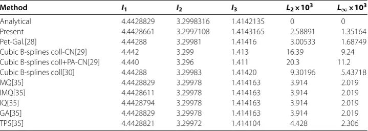
Table 2 Errors and invariants for a single solitary wave withc= 1,h= 0.2,k= 0.025, 0≤x≤100, att= 10
Method I1 I2 I3 L2×103 L∞×103
Analytical 4.4428829 3.2998316 1.4142135 0 0
Present 4.4428661 3.2997108 1.4143165 2.58891 1.35164
Pet-Gal.[28] 4.44288 3.29981 1.41416 3.00533 1.68749
Cubic B-splines coll-CN[29] 4.442 3.299 1.413 16.39 9.24 Cubic B-splines coll+PA-CN[29] 4.440 3.296 1.411 20.3 11.2 Cubic B-splines coll[30] 4.44288 3.29983 1.41420 9.30196 5.43718
MQ[35] 4.4428829 3.29978 1.414163 3.914 2.019
IMQ[35] 4.4428611 3.29978 1.414163 3.914 2.019
IQ[35] 4.4428794 3.29978 1.414163 3.914 2.019
GA[35] 4.4428829 3.29978 1.414163 3.914 2.019
TPS[35] 4.4428821 3.29972 1.414104 4.428 2.306
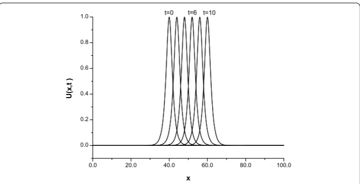
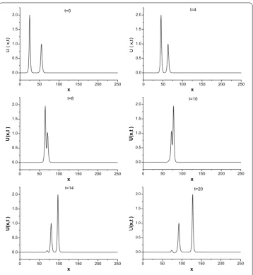
and the computed values of invariants are in good agreement with their analytical val-uesI= .,I= .,I= .. Percentage values of the relative er-ror of the conserved quantitiesI,IandIare calculated with respect to the conserved quantities att= . Percentage values of relative changes ofI,I andI are found to be .×–%, .×–%, .×–%, respectively. Thus, the invariants remain almost constant during the computer run. Table displays a comparison of the values of the invariants and error norms obtained by the present method with those obtained by other methods [–, ]. It can be seen from Table that the error norms obtained by the present method are smaller than other methods [–, ]. Figure shows the motion of a solitary wave withc= ,h= .,k= . at different time levels. It is ob-served that the soliton moves to the right at a constant speed and almost unchanged am-plitude with increasing time, as expected. Att= the amplitude is . which is located atx= , while it is . which is located atx= . At timest= andt= , the absolute difference in amplitude is ×–so there is a little change between the ampli-tudes.
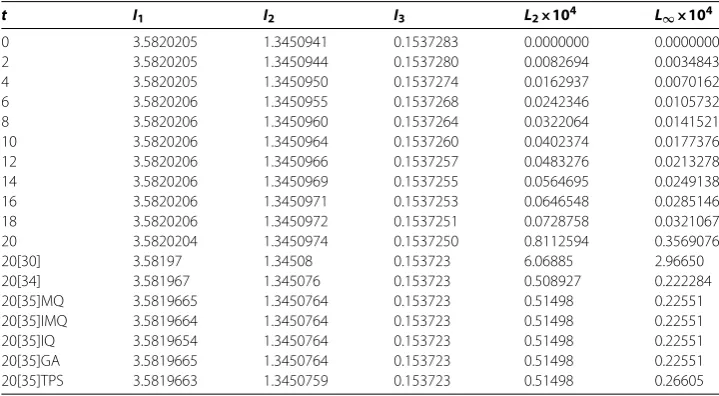
For the second set, the parametersμ= ,c= .,h= .,k= . andx= with range [, ] are chosen to compare the results obtained by the present method with those obtained given in Refs. [, , , , ]. So, the solitary wave has amplitude . and the computations are done up to timet= to obtain the invariants and error norms
Figure 1 Single solitary wave withc= 1,h= 0.2,t= 0.025, 0≤x≤100,t= 0, 2, 4, 6, 8 and 10.
given in Refs. [, ] and almost the same as those in Refs. [, , ]. The agreement between numerical and analytic solutions is perfect which is given by Eq. . Percentage values of relative changes ofI,IandIare found to be .×–%, .×–%, .×–%, respectively. Moreover, from Table , the changing of the invariantsI
,I andIduring the computer run is less than ×–, .×–, .×–, respectively. The profiles of the solitary wave at different time levels have been shown in Figure . The distributions of the errors at timet= andt= are shown graphically for solitary wave amplitudes and . in Figure . It is seen that the maximum errors are about at the tip of the solitary waves and between –×–and ×–, –×– and ×–, respectively.
3.2 Interaction of two solitary waves
Here the interaction of two solitary waves is studied by using the initial condition given by the linear sum of two well-separated solitary waves having various amplitudes
U(x, ) =
j=
Ajsech
pj(x–xj)
, ()
whereAj=√cj,pj=
c
j
μ(cj+),j= , ,cjandxjare arbitrary constants. The analytical values
of the invariants are found by []
I=
j= π√cj
pj ,
I=
j=
cj
pj
+μpjcj
,
I=
j=
c j pj
–μpjcj
.
Table 3 Invariants and error norms for a single solitary wave withc= 0.3,h= 0.1,k= 0.01, 0≤x≤100
t I1 I2 I3 L2×104 L∞×104
0 3.5820205 1.3450941 0.1537283 0.0000000 0.0000000
2 3.5820205 1.3450944 0.1537280 0.0082694 0.0034843
4 3.5820205 1.3450950 0.1537274 0.0162937 0.0070162
6 3.5820206 1.3450955 0.1537268 0.0242346 0.0105732
8 3.5820206 1.3450960 0.1537264 0.0322064 0.0141521
10 3.5820206 1.3450964 0.1537260 0.0402374 0.0177376
12 3.5820206 1.3450966 0.1537257 0.0483276 0.0213278
14 3.5820206 1.3450969 0.1537255 0.0564695 0.0249138
16 3.5820206 1.3450971 0.1537253 0.0646548 0.0285146
18 3.5820206 1.3450972 0.1537251 0.0728758 0.0321067
20 3.5820204 1.3450974 0.1537250 0.8112594 0.3569076
20[30] 3.58197 1.34508 0.153723 6.06885 2.96650
20[34] 3.581967 1.345076 0.153723 0.508927 0.222284
20[35]MQ 3.5819665 1.3450764 0.153723 0.51498 0.22551
20[35]IMQ 3.5819664 1.3450764 0.153723 0.51498 0.22551
20[35]IQ 3.5819654 1.3450764 0.153723 0.51498 0.22551
20[35]GA 3.5819665 1.3450764 0.153723 0.51498 0.22551
20[35]TPS 3.5819663 1.3450759 0.153723 0.51498 0.26605
Figure 2 Single solitary wave withc= 0.3,h= 0.1,t= 0.01, 0≤x≤100 at timest= 0, 5, 10, 15 and 20.
Table 4 Comparison of invariants for the interaction of two solitary waves with results from [34] withh= 0.2,k= 0.025 in the region 0≤x≤250
Present method [34]
t I1 I2 I3 I1 I2 I3
0 11.4676542 14.6292080 22.8803584 11.467698 14.629277 22.880432 2 11.4678169 14.6282301 22.8813363 11.467698 14.624259 22.860365 4 11.4679819 14.6282293 22.8813371 11.467698 14.619226 22.840279 6 11.4681349 14.6181053 22.8914611 11.467699 14.614169 22.820069 8 11.4675390 14.1393389 23.3702275 11.467700 14.606821 22.787857 10 11.4674118 14.0502062 23.4593602 11.467700 14.603687 22.771773 12 11.4685494 14.6816556 22.8279107 11.467699 14.603056 22.775766 14 11.4687073 14.6648742 22.8446922 11.467699 14.598059 22.756029 16 11.4688627 14.6459207 22.8636457 11.467700 14.593048 22.736127 18 11.4690242 14.6370095 22.8725569 11.467700 14.588061 22.716289 20 11.4691886 14.6331334 22.8764330 11.467701 14.583089 22.696510 20[28] 11.4677 14.6299 22.8806
20[30] 11.4677 14.6292 22.8809 20[35]MQ 11.467698 14.583052 22.696539 20[35]IMQ 11.467679 14.583052 22.696539 20[35]IQ 11.467690 14.583052 22.696539 20[35]GA 11.467698 14.583052 22.696539 20[35]TPS 11.467742 14.582424 22.694269
For the numerical simulation, the parameters μ= , h= .,k= .,c= ,c= ,
x= ,x= are used over the range ≤x≤ to coincide with those used by Refs. [, , , ]. The experiment is run fromt= tot= and the values of invariant quantitiesI,IandIare recorded in Table . The analytical values of the invariants for this case areI= .,I= .,I= .. A comparison of the values of the invariants obtained by the present method with those obtained in Refs. [, , , ] are listed in Table . It is seen that the obtained values of the invariants remain almost constant during the computer run. The development of the interaction of two soli-tary waves is shown in Figure . It can be seen from the figure that att= the wave with larger amplitude is to the left of the second wave with smaller amplitude. Since the taller wave moves faster than the shorter one, it catches up and collides with the shorter one att= and then moves away from the shorter one as time increases. Att= , the am-plitude of larger waves is . at the pointx= . whereas the amplitude of the smaller one is . at the pointx= . It is found that the absolute difference in am-plitude is .×– for the smaller wave and .×– for the larger wave for this algorithm.
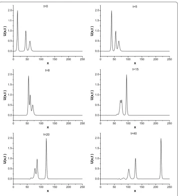
3.3 Interaction of three solitary waves
For this problem, the behavior of interaction of three solitary waves having different am-plitudes and traveling in the same direction is studied. So, we consider Eq. () with the initial condition given by the linear sum of three well-separated solitary waves of different amplitudes
U(x, ) =
j=
Ajsech
pj(x–xj)
Figure 4 Interaction of two solitary waves witht= 0, 4, 8, 10, 14, 20.
whereAj=√cj, pj=
c
j
μ(cj+),j= , , ,cj andxj are arbitrary constants. The analytical
values of the conservation laws are found from Eq. () as follows:
I=
j= π√cj
pj ,
I=
j=
cj
pj
+μpjcj
,
I=
j=
c j pj
–μpjcj
.
()
For the purpose of comparison, parameters μ= , h= ., k= .,c = ,c= ,
Table 5 Comparison of invariants for the interaction of three solitary waves with results from [34] withh= 0.2,k= 0.025 in the region 0≤x≤250
Present method [34]
t I1 I2 I3 I1 I2 I3
0 14.9800762 15.8374849 23.0081806 14.980099 15.837528 23.008136 5 14.9381371 15.7382326 23.1074329 14.980105 15.824928 22.957891 10 14.9071292 14.1781087 24.6675567 14.980109 15.807025 22.877972 15 14.8836886 15.3648852 23.4807802 14.980106 15.807032 22.885947 20 14.8503851 15.5659364 23.2797291 14.980106 15.795022 22.837454 25 14.8194163 15.6235556 23.2221098 14.980107 15.782840 22.788852 30 14.7905616 15.5976717 23.2479938 14.980107 15.770634 22.740419 35 14.7636015 15.5610664 23.2845991 14.980108 15.758480 22.692279 40 14.7383184 15.5256320 23.3200335 14.980108 15.746389 22.644448 45 14.7145273 15.4927592 23.3529062 14.968030 15.734374 22.596591 45[30] 13.7043 15.6563 22.9303
45[35]MQ 14.96814 15.73434 22.596625 45[35]IMQ 14.96808 15.73434 22.596625 45[35]IQ 14.96813 15.73434 22.596625 45[35]GA 14.96810 15.73433 22.596626 45[35]TPS 14.96824 15.73376 22.594494
obtained by the present method with those obtained in Refs. [, , ] are shown in Ta-ble . It is observed from the taTa-ble that the obtained values of the invariants remain almost constant during the computer run which are all in good agreement with their analytical values given by Eq. (). The absolute difference between the values of the conservative constants obtained by the present method at timest= andt= areI= .×–, I= .×–,I= .×–, respectively. Figure shows the interaction of these solitary waves at different times. As it is seen from the Figure , the interaction started at about timet= , overlapping processes occurred between timet= andt= and waves started to resume their original shapes after the timet= .
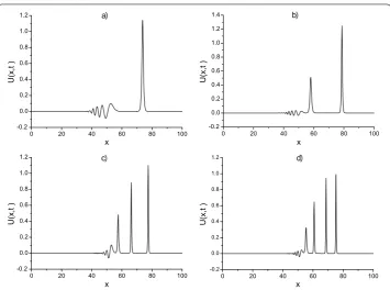
3.4 The Maxwellian initial condition
Finally, we have studied the development of the Maxwellian initial condition
U(x, ) =exp–(x– ) ()
into a train of solitary waves. As it is known, with the Maxwellian condition (), the be-havior of the solution depends on the values ofμ. We study each of the following cases: μ= .,μ= .,μ= . and μ= .. For μ= ., only a single soliton is formed as shown in Figure a. Whenμ= . andμ= ., two and three stable solitons are formed, respectively, as shown in Figure b, c. Forμ= ., the Maxwellian initial condi-tion has decayed into four solitary waves as shown in Figure d. All figures were drawn up at timet= .. The peaks of the well-developed wave lie on a straight line, so that their ve-locities are linearly dependent on their amplitudes. We also observe a small oscillating tail appearing behind the last wave in all Maxwellian figures. The obtained numerical values of the invariants are given in Table .
4 Conclusions
Figure 5 Interaction of three solitary waves witht= 0, 5, 8, 15, 20, 40.
Table 6 Invariants of the MRLW equation using the Maxwellian initial condition
t μ I1 I2 I3 μ I1 I2 I3
0 0.1 1.7724809 1.3786633 0.7609104 0.015 1.7724809 1.2721327 0.8674410 3 1.7721927 1.4728222 0.6667515 1.7436793 1.4180550 0.7215188 6 1.7717480 1.4720618 0.6675119 1.7244620 1.4036726 0.7359011 9 1.7713064 1.4715473 0.6680264 1.7116986 1.3940073 0.7455664 12 1.7708674 1.4711193 0.6684544 1.7021509 1.3870669 0.7525068 15 1.7704309 1.4707290 0.6688447 1.6945087 1.3816736 0.7579001 0 0.01 1.7724809 1.2658662 0.8737075 0.04 1.7724809 1.3034651 0.8361087 3 1.7264258 1.4001430 0.7394307 1.7685556 1.4501960 0.6893777 6 1.7031386 1.3850514 0.7545223 1.7637294 1.4456393 0.6939344 9 1.6885258 1.3755380 0.7640357 1.7592882 1.4415131 0.6980606 12 1.6777156 1.3686563 0.7709174 1.7551780 1.4378815 0.7016922 15 1.6691476 1.3635304 0.7760434 1.7513552 1.4345989 0.7049748
Figure 6 Maxwellian initial condition att= 14.5 with a)μ= 0.1, b)μ= 0.04, c)μ= 0.015, d)μ= 0.01.
been used. It is seen that the error norms are sufficiently small and the invariants are well conserved. The method successfully models the motion and interaction of solitary waves. The computed results indicate that the present method is more accurate than some earlier results found in the literature. So, it can be said that the method is a reliable one for ob-taining the numerical solutions of a wider range of physically important non-linear partial differential equations.
Competing interests
The authors declare that they have no competing interests. Authors’ contributions
All the three authors have almost equal contributions to the article. In particular, SBGK participated in the design of the basic outline of the article and equations. NMY participated in the application of the method and obtaining the iterative formulae. YU participated in coding and running the necessary programs. All authors worked together to check and test the programs, to obtain the results, to carry out the literature search. All authors read, checked, corrected and approved the final manuscript.
Author details
1Department of Mathematics, Faculty of Science and Art, Nevsehir University, Nevsehir, 50300, Turkey.2Department of Mathematics, Faculty of Science and Art, Inönü University, Malatya, 44280, Turkey.
Acknowledgements
Dedicated to Professor Hari M Srivastava.
The authors would like to thank the reviewers for their careful reading and making some useful comments which improved the presentation of the paper.
Received: 19 November 2012 Accepted: 29 January 2013 Published: 14 February 2013
References
1. Peregrine, DH: Calculations of the development of an undular bore. J. Fluid Mech.25, 321-330 (1966)
2. Bona, JL, Pryant, PJ: A mathematical model for long wave generated by wave makers in nonlinear dispersive systems. Proc. Camb. Philos. Soc.73, 391-405 (1973)
4. Morrison, PJ, Meiss, JD, Cary, JA: Scattering of regularized long wave solitary waves. Physica11D, 324-336 (1984) 5. Eilbeck, JC, McGuire, GR: Numerical study of the regularized long wave equation, II: Interaction of solitary wave.
J. Comput. Phys.23, 63-73 (1977)
6. Jain, PC, Shankar, R, Singh, TV: Numerical solution of regularized long wave equation. Commun. Numer. Methods Eng.9, 579-586 (1993)
7. Bhardwaj, D, Shankar, R: A computational method for regularized long wave equation. Comput. Math. Appl.40, 1397-1404 (2000)
8. Chang, Q, Wang, G, Guo, B: Conservative scheme for a model of nonlinear dispersive waves and its solitary waves induced by boundary motion. J. Comput. Phys.93, 360-375 (1995)
9. Gardner, LRT, Gardner, GA: Solitary waves of the regularized long wave equation. J. Comput. Phys.91, 441-459 (1990) 10. Gardner, LRT, Gardner, GA, Dogan, A: A least-squares finite element scheme for the RLW equation. Commun. Numer.
Methods Eng.12, 795-804 (1996)
11. Gardner, LRT, Gardner, GA, Dag, I: A B-spline finite element method for the regularized long wave equation. Commun. Numer. Methods Eng.11, 59-68 (1995)
12. Alexander, ME, Morris, JL: Galerkin method applied to some model equations for nonlinear dispersive waves. J. Comput. Phys.30, 428-451 (1979)
13. Serna, JMS, Christie, I: Petrov Galerkin methods for nonlinear dispersive wave. J. Comput. Phys.39, 94-102 (1981) 14. Dogan, A: Numerical solution of RLW equation using linear finite elements within Galerkin’s method. Appl. Math.
Model.26, 771-783 (2002)
15. Esen, A, Kutluay, S: Application of lumped Galerkin method to the regularized long wave equation. Appl. Math. Comput.174(2), 833-845 (2006)
16. Soliman, AA, Raslan, KR: Collocation method using quadratic b-spline for the RLW equation. Int. J. Comput. Math.78, 399-412 (2001)
17. Soliman, AA, Hussien, MH: Collocation solution for RLW equation with septic spline. Appl. Math. Comput.161, 623-636 (2005)
18. Raslan, KR: A computational method for the regularized long wave (RLW) equation. Appl. Math. Comput.167, 1101-1118 (2005)
19. Saka, B, Dag, I, Dogan, A: Galerkin method for the numerical solution of the RLW equation using quadratic B-splines. Int. J. Comput. Math.81(6), 727-739 (2004)
20. Dag, I, Saka, B, Irk, D: Application of cubic B-splines for numerical solution of the RLW equation. Appl. Math. Comput.
159, 373-389 (2004)
21. Dag, I, Ozer, MN: Approximation of RLW equation by least-square cubic B-spline finite element method. Appl. Math. Model.25, 221-231 (2001)
22. Zaki, SI: Solitary waves of the splitted RLW equation. Comput. Phys. Commun.138, 80-91 (2001)
23. Gou, BY, Cao, WM: The Fourier pseudo-spectral method with a restrain operator for the RLW equation. J. Comput. Phys.74, 110-126 (1988)
24. Islam, S, Haq, F, Ali, A: A meshfree method for the numerical solution of the RLW equation. J. Comput. Appl. Math.
223, 997-1012 (2009)
25. Zhang, L: A finite difference scheme for generalized long wave equation. Appl. Math. Comput.168(2), 962-972 (2005) 26. Ramos, JI: Solitary wave interactions of the GRLW equation. Chaos Solitons Fractals33, 479-491 (2007)
27. Kaya, D, El-Sayed, SM: An application of the decomposition method for the generalized KdV and RLW equations. Chaos Solitons Fractals17, 869-877 (2003)
28. Roshan, T: A Petrov-Galerkin method for solving the generalized regularized long wave (GRLW) equation. Comput. Math. Appl.63, 943-956 (2012)
29. Gardner, LRT, Gardner, GA, Ayoup, FA, Amein, NK: Simulations of solitary waves of the MRLW equation by B-spline finite element. Arab. J. Sci. Eng.22, 183-193 (1997)
30. Khalifa, AK, Raslan, KR, Alzubaidi, HM: A collocation method with cubic B-splines for solving the MRLW equation. J. Comput. Appl. Math.212, 406-418 (2008)
31. Khalifa, AK, Raslan, KR, Alzubaidi, HM: A finite difference scheme for the MRLW and solitary wave interactions. Appl. Math. Comput.189, 346-354 (2007)
32. Raslan, KR: Numerical study of the modified regularized long wave equation. Chaos Solitons Fractals42, 1845-1853 (2009)
33. Raslan, KR, Hassan, SM: Solitary waves for the MRLW equation. Appl. Math. Lett.22, 984-989 (2009)
34. Haq, F, Islam, S, Tirmizi, IA: A numerical technique for solution of the MRLW equation using quartic B-splines. Appl. Math. Model.34, 4151-4160 (2010)
35. Ali, A: Mesh free collocation method for numerical solution of initial-boundary value problems using radial basis functions. Dissertation, Ghulam Ishaq Khan Institute of Engineering Sciences and Technology (2009)
36. Rubin, SG, Graves, RA: Cubic spline approximation for problems in fluid mechanics. Nasa TR R-436, Washington DC (1975)
37. Prenter, PM: Splines and Variational Methods. Wiley, New York (1975)
38. Olver, PJ: Euler operators and conservation laws of the BBM equation. Math. Proc. Camb. Philos. Soc.85, 143-159 (1979)
doi:10.1186/1687-2770-2013-27
![Table 4 Comparison of invariants for the interaction of two solitary waves with results from[34] with h = 0.2, k = 0.025 in the region 0 ≤ x ≤ 250](https://thumb-us.123doks.com/thumbv2/123dok_us/483974.2047266/12.595.121.477.108.318/table-comparison-invariants-interaction-solitary-waves-results-region.webp)
![Table 5 Comparison of invariants for the interaction of three solitary waves with results from[34] with h = 0.2, k = 0.025 in the region 0 ≤ x ≤ 250](https://thumb-us.123doks.com/thumbv2/123dok_us/483974.2047266/14.595.118.478.108.300/table-comparison-invariants-interaction-solitary-waves-results-region.webp)