DECOMPOSITION METHOD IN COMPARISON WITH NUMERICAL SOLUTIONS OF BURGERS EQUATION

(1)

DECOMPOSITION METHOD IN

COMPARISON WITH NUMERICAL

SOLUTIONS OF BURGERS EQUATION

Christos Mamaloukas*_{and Stefanos Spartalis}**

ABSTRACT – This paper presents a solution of the one-dimension Burgers equation using Decomposition Method and compares this solution to the analytic solution [Cole] and solutions obtained with other numerical methods. Even though decomposition method is a non-numerical method, it can be adapted for solving nonlinear differential equations. The advantage of this methodology is that it leads to an analytical continuous approximated solution that is very rapidly convergent [2,7,8]. This method does not take any help of linearization or any other simplifications for handling the non-linear terms. Since the decomposition parameter, in general, is not a perturbation parameter, it follows that the non-linearities in the operator equation can be handled easily, and accurate solution may be obtained for any physical problem.

1. Introduction

Many problems in Fluid Mechanics and in Physics are governed generally by the Navier-Stokes equations. These equations can show the behaviour of a certain attribute (e.g. momentum, heat) in space and time. The one-dimension non-linear differential equation which is used as a model for these problems is Burgers equation. This equation is applied to laminar and turbulence flows as

*

Athens University of Economics and Business, Dept. of Informatics, 76 Patision Str, 10434 Athens, Greece, email: [email protected]

**

(2)

well. The Burgers equation which is the one-dimension nonlinear Diffusion Equation is similar to the one dimension Navier-Stokes equation without the stress term. Many researchers tried to find analytic and numerical solutions of this equation using the appropriate initial and boundary conditions. Characteristically in Benton and Platzman [10] are mentioned almost 35 distinct solutions of Burger equation but only the half of them are having physical interest. Agas [9] tried to get approximate solution of Burger equation using a new numerical solution which is called “Group of Explicit” Method. He also tried the method of Finite Differences and the method of Lines in Finite Elements. The problem he faced was that these methods could not give solutions for big values of the Reynolds number. He also found some problems in convergence.

In this paper, a solution obtained by the Adomian's Decomposition Method (ADM), which is described briefly in this paper and was used by Mamaloukas [12, 13] for the numerical solution of the one-dimensional Kortweg-de Vries equation and the pulsatile flow of an incompressible viscous fluid through a circular rigid tube provided with constriction, is compared numerically and graphically to the analytic and to some others numerical methods. As it is shown in the diagrams at the end of this paper this method gives a computable and accurate solution of the problem using only a small number of terms.

2. Formulation of the Problem

Consider the Burgers equation with the following form 2

2

u u u

u

t x  x

  

 

   (1)

with boundary conditions: (0, )u t u(1, )t 0for t0 (2)

and initial condition: ( , 0)u x 4 (1x x or) sinx (3)

3. Brief Description of ADM

Let

2 2 and

t xx

L L

t x

 

 

  . Then the equation (1) takes the form:

t xx

(3)

where the first term is the linear, the third is the highest order term and the second is the non-linear term given by

u Nu u x    (5)

Now, solving (4) for L ut and L uxx correspondingly we have t xx

L uL uNu (6)

1





xx t

L u  L u Nu

 

(7)

By defining the one and twofold right-inverse operators 1 1 and

t xx

L L

, given by

the form 1

 

1

 

and

t xx

L 

_

 dt L 

_

 dx dx, we can formally obtain from (6) and (7)





1 1

t t t xx

L L u L L u Nu

  (8)





1 1 1

xx xx xx t

L L u L L u Nu

  (9)

From relations (8) and (9) we obtain









1 1 1

0 1

2 xx t t xx

uu  _L L uNu L L uNu _ (10) where the term u₀ is to be determined from the initial conditions, so, is

u0 4 (1x x or) sinx (11)

4. Solution of Burger's Equation with ADM

Now, we introduce a formal counting parameter λ to write equation (10) in the following form









1 1 1

0 1

2 xx t t xx

u u  L L u Nu L L u Nu

 

  _    _ (12)

(4)

0

n n n

u  u

 



_

(13)

0

n n n

N u  A

 



_

(14)

where A_n are the Adomian’s special polynomials [1,2] for the specific non-linearity to be determined by expanding Nu in the ascending power of λ and equating the terms of like powers of λ from both sides of (12). These special polynomials depend only on the u0 to un components.

Substituting the expressions (13) and (14) into (12) and then equating the like power terms from both sides of the resulting expression we have

























1 1 1

1 0 0 0 0

1 1 1

2 1 1 1 1

1 1 1

1 1 2 1 2 ... 1 , 0, 2

xx t t xx

n xx t n n t xx n n

u L L u A L L u A

u L L u A L L u A n

                   _    _    _    _  

 _    _  1, 2,...,n

(15)

All components are determinable since A₀ depends only on u₀, A₁ depends only on u u0, 1,…, An depends only on u0,u1, ...,un. So, in order to determine

Adomian’s special polynomials, from (5) and (14) we write

0 n n n

u

A

u

x



 









(16)

Substituting (13) into (16) and then comparing like-power terms of λ on both sides of resulting expression we obtain the following polynomials.

0 0 0

0 1

1 0 1

0

2 1

2 0 1 2

... ... u A u x u u

A u u

x x

u

u u

A u u u

x x x

              

(5)

Using the initial condition (11) A0 can be calculated from expression (17). Substituting the result in the expression of u1 (15) and then performing all necessary calculations and integrations with respect to t and x respectively, we have u₁ which is:

3 5

2 3 4

1

4 4

4 8 24 16 2

3 5

v x v x

u   v t t x t x   t x  v x  (18)

and u₂ which is

3

2 2 2 2 2 2 2 2 2 2

2

5

3 2 3 2 3 4 4 2 4

2 5 2 6 2 7 2 8

5 6

2

16 4 16 32 16 96

3

32 148 2

16 160 80

3 3 5

8 248 10 248 4

15 5 9 15 5 5

v x u v t v t x t x v t x v x v t x t x

v x v t x v t x t x v x v t x t x v x v x v x v x

v t x v t x

        

       

     

(19)

If we suggest as a solution of u an approximation of only two or three terms then from (11), (18) and (19) we have the solution of (1):

0 1

uu u or uu0u1u2

As an example, if we give the values x0.25,t0.05,v0.001 we get 0.712314

u with two terms and u0.712791 with three terms.

5. Tables of Results and Diagrams

For the solution of this equation the initial conditions ( , 0)u x 4 (1x x) and ( , 0) sin

(6)

In the above diagrams numerical results of Burger equation are registered for different values of v. For comparison reasons the viscosity values

1, 0.1, 0.01, 0.001

v v v v were used.

(7)

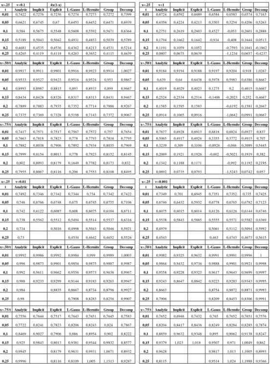
Table 1: Comparison results for Burger equation for initial condition 4 (1x x) with 1, 0.1, 0.01, 0.001, 0.25, 0.05

v  x  t

x=.25 v=0.1 4x(1-x) x=.25 v=1 t Analytic Implicit Explicit L-Gauss L-Hermite Group Decomp t Analytic Implicit Explicit L-Gauss L-Hermite Group Decomp 0,01 0,7422 0,7276 0,7236 0,7274 0,7273 0,7272 0,7399 0,01 0,6724 0,6592 0,6489 0,6584 0,6583 0,6574 0,7163

0,05 0,6621 0,6745 0,67 0,6453 0,6452 0,6471 0,6939 0,05 0,4356 0,4224 0,4213 0,3503 0,3254 0,4206 0,5263

0,1 0,584 0,5675 0,5548 0,5608 0,5592 0,5671 0,6364 0,1 0,2751 0,2619 0,2603 0,4527 -0,053 0,2601 0,2888

0,15 0,5189 0,5043 0,5042 0,4931 0,4853 0,5039 0,5789 0,15 0,1794 0,1662 0,1642 -0,934 -0,408 0,1644 0,0513

0,2 0,4681 0,4535 0,4536 0,4362 0,4213 0,4531 0,5214 0,2 0,1191 0,1059 0,1052 -0,7593 0,1041 -0,1862

0,25 0,4265 0,4119 0,4118 0,4263 0,3652 0,4115 0,4639 0,25 0,0807 0,0675 0,0639 -1,1234 0,0657 -0,4237

x=.50/t Analytic Implicit Explicit L-Gauss L-Hermite Group Decomp x=.50/t Analytic Implicit Explicit L-Gauss L-Hermite Group Decomp 0,01 0,9917 0,9911 0,9901 0,9916 0,9923 0,9914 1,0027 0,01 0,9184 0,9194 0,9188 0,9197 0,9204 0,918 1,0267

0,05 0,9533 0,9527 0,9423 0,9516 0,9524 0,953 0,9867 0,05 0,639 0,64 0,6438 0,5978 0,5983 0,6386 0,8667

0,1 0,8993 0,8987 0,8815 0,893 0,8933 0,899 0,9667 0,1 0,4019 0,4029 0,4023 0,1275 0,2 0,4015 0,6667

0,15 0,8434 0,8428 0,8326 0,8317 0,8313 0,8431 0,9467 0,15 0,2524 0,2534 0,2514 -0,1408 -0,2023 0,252 0,4667

0,2 0,7889 0,7883 0,7935 0,7352 0,7714 0,7886 0,9267 0,2 0,1585 0,1595 0,1583 -0,6192 0,1581 0,2667

0,25 0,7375 0,7369 0,7328 0,5198 0,7143 0,7372 0,9067 0,25 0,0914 0,1065 0,0916 -1,0642 0,0991 0,0667

0,05 0,7663 0,7818 0,7823 0,778 0,7793 0,7816 0,7795 0,05 0,5065 0,4917 0,4924 0,3355 0,3772 0,4915 0,707

0,1 0,7882 0,8038 0,7906 0,7892 0,7934 0,8035 0,7969 0,1 0,3239 0,309 0,3106 -0,8926 -0,046 0,3089 0,5445

0,15 0,7999 0,8154 0,8013 0,778 0,7923 0,8152 0,8145 0,15 0,2069 0,1921 0,1926 -0,602 -0,5021 0,1919 0,382

0,2 0,802 0,8093 0,8179 0,1649 0,7782 0,8173 0,832 0,2 0,1342 0,1188 0,1171 -0,992 0,1192 0,2195

0,25 0,7955 0,8067 0,8116 0,206 0,7553 0,8108 0,8495 0,25 0,0892 0,0735 0,0793 -1,5243 0,0742 0,057

x=.25 v=0.01 x=.25 v=0.001 t Analytic Implicit Explicit L-Gauss L-Hermite Group Decomp t Analytic Implicit Explicit L-Gauss L-Hermite Group Decomp 0,01 0,7492 0,7346 0,7342 0,7344 0,734 0,7342 0,7422 0,01 0,7349 0,701 0,6945 0,7351 0,7352 0,735 0,7425

0,05 0,746 0,6766 0,6748 0,675 0,6745 0,6755 0,7106 0,05 0,6746 0,6432 0,5932 0,6778 0,6765 0,6782 0,7123

0,1 0,742 0,6122 0,6087 0,608 0,6075 0,6104 0,6711 0,1 0,6075 0,6015 0,6014 0,6126 0,6126 0,6144 0,6746

0,15 0,738 0,5562 0,5512 0,5494 0,5514 0,5537 0,6316 0,15 0,5538 0,5843 0,5885 0,5555 0,5571 0,5582 0,6369

0,2 0,734 0,5016 0,4998 0,5043 0,5046 0,5921 0,2 0,4979 0,5061 0,5112 0,5094 0,5992

0,25 0,73 0,4534 0,4642 0,4652 0,5526 0,25 0,4543 0,463 0,4743 0,4673 0,5615

x=.50/t Analytic Implicit Explicit L-Gauss L-Hermite Group Decomp x=.50/t Analytic Implicit Explicit L-Gauss L-Hermite Group Decomp 0,01 0,9992 0,9986 0,9992 0,9984 0,999 0,9989 1,0003 0,01 0,9982 0,9325 0,9632 0,9991 0,9991 0,9996 1

0,05 0,996 0,9873 0,9901 0,9854 0,9875 0,9887 0,9987 0,05 0,9864 0,9432 0,9736 0,9888 0,9901 0,9921 0,9998

0,1 0,992 0,9611 0,9662 0,9556 0,9573 0,9636 0,9967 0,1 0,9558 0,9228 0,9323 0,9617 0,9643 0,9699 0,9997

0,15 0,988 0,9233 0,9299 0,9144 0,9183 0,9263 0,9947 0,15 0,9243 0,8647 0,8842 0,9223 0,9283 0,9343 0,9995

0,2 0,984 0,8835 0,8667 0,8734 0,8796 0,9927 0,2 0,8663 0,8754 0,8872 0,8871 0,9993

0,25 0,98 0,7908 0,8283 0,8256 0,9907 0,25 0,7906 0,8209 0,8453 0,8306 0,9991

0,05 0,7722 0,8241 0,7823 0,8206 0,8243 0,824 0,7867 0,05 0,8204 0,8417 0,8436 0,8249 0,8284 0,8285 0,7874

0,1 0,8469 0,9027 0,7906 0,886 0,8954 0,902 0,8222 0,1 0,8859 0,9632 0,9348 0,895 0,9062 0,9138 0,8247

0,15 0,925 0,9843 0,8013 0,9381 0,9544 0,9832 0,8577 0,15 0,9379 1,023 1,018 0,9507 0,971 1,0049 0,862

0,2 0,9945 0,8179 0,9631 0,9931 1,0671 0,8932 0,2 0,9628 0,9817 1,013 1,1005 0,8993

(8)

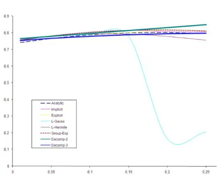
Diagram 1: Comparison results with v1, x0.25, 0.01 t 0.25 using 2 and 3 terms

(9)

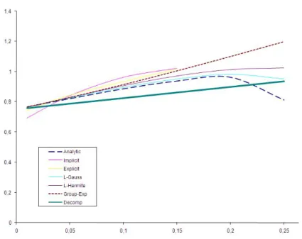
Diagram 3: Comparison results with v0.1,x0.75, 0.01 t 0.25 using 2 and 3 terms

(10)

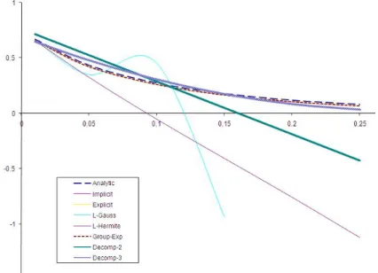
Diagram 5: Comparison results with v0.001,x0.75, 0.01 t 0.25 and 2 terms

6. Discussions

The analytic solution as it is described by Cole [13] is liable to restrictions concerning the values of the coefficient 1

e

v R

 . For example, if the value of the Reynolds number is greater than 1000 then we can not find any solution because Fourier series do not converge. For this reason we try numerical approaches, like finite differences and finite elements.

Concerning finite differences the explicit method give us adequate results if and only if 1 / 2. Otherwise results did not converge. With the implicit method we do not need the covenant 1 / 2, but we need a large number of calculations. Finally, the group of explicit methods gives us adequate results with few calculations and the method is more stable.

(11)

Concerning the decomposition method from the above diagrams it is obvious how powerful this method is. Using only two terms we can obtain similar results with the other numerical methods and the analytic solution. Of course, in some cases the present solutions deviate from the solutions given in the table. The decomposition solution can be further improved if more-term approximations of the solution are obtained.

As far as accurate results are concerned, computational experience has shown that they can be obtained easily by taking half a dozen terms. In case we do not have a sufficiently high precision by using a few of the An, then accordingly to

Rach R. [15] there are two alternatives. One is to compute additional terms by any of the available procedures. The second approach is to use the Adomian-Malakian ''convergence acceleration'' procedure [16]. This unique approach conveniently yields the error-damping effect of calculating many more terms of the An to determine whether further calculation is required.

7. Conclusions

The great advantage of the decomposition method is that of avoiding simplifications and restrictions which change the non-linear problem into a mathematically tractable one, whose solution is not consistent to physical solution.

Further study on the stability and the convergence of the solutions will prove the accuracy of the above method.

BIBLIOGRAPHY

1. G. ADOMIAN, Nonlinear Stochastic Operator Equations, Academic Press, 1986.

2. G. ADOMIAN, Nonlinear Stochastic Systems Theory and Applications to

Physics, Kluwer Academic Publishers, 1989.

3. G. ADOMIAN, J. Math. Anal. Appl., 119, (1986), 340-360. 4. G. ADOMIAN, Appld. Math. Lett., 6, No5, (1993), 35-36.

5. G. ADOMIAN, Rach R., On the Solution of Nonlinear Differential Equations with Convolution Product Non-linearities, J. Math. Anal. Appl., 114, (1986), 171-175.

6. G. ADOMIAN, Solving Frontier Problems of Physics: The Decomposition

Method, Kluwer Academic Publishers, 1994.

7. Y. CHERRUAULT, Kybernetes, 18, No2, (1989), 31-39.

8. Y. CHERRUAULT, Math. Comp. Modeling, 16, No2, (1992), 85-93. 9. C. AGAS, The Effect of Kinematic Viscosity in the Numerical Solution of

(12)

10. E.R. BENTON & G.W. PLATZMAN, A Table of Solutions of the

one-dimensional Burgers Equation, Quart. Appl. Math., 1972.

11. J. M. BURGERS, The Nonlinear Diffusion Equation, D. Reidel Publishing Company, Univ. of Maryland, USA, 1974.

12. C. MAMALOUKAS, Numerical Solution of one dimensional Kortweg-de

Vries Equation, BSG Proceedings 6, Global Analysis, Differential

Geometry and Lie Algebras, 6, (2001), 130-140.

13. C. MAMALOUKAS, Haldar K., Mazumdar H. P., Application of double decomposition to pulsatile flow, Journal of Computational & Applied Mathematics, 10 , Issue 1-2, (2002), 193–207.

14. J.D. COLE, On a Quasilinear Parabolic Equation Occurring in

Aerodynamics, A.Appl. Maths, 9, (1951), 225-236.

15. N. K. MADSEN and R. F. SINCOVEC, General Software for Partial Differential Equations in Numerical Methods for Differential System, Ed. Lapidus L., and Schiesser W. E., Academic Press, Inc., 1976.

16. R. RACH, A Convenient Computational Form of the Adomian Polynomials, J. Math. Anal. Appl., 102, (1984), 415-419.

17. G. ADOMIAN and MALAKIAN, Self-correcting approximate solutions by the iterative method for nonlinear Stochastic Differential Equations, J. Math. Anal. Appl., 76, (1980), 309-327.

18. G. ADOMIAN and MALAKIAN, Inversion of Stochastic Partial Differential Operators-The Linear Case, J. Math. Anal. Appl., 77, (1980), 505-512.

19. G. ADOMIAN and MALAKIAN, Existence of the Inverse of a Linear Stochastic Operator, J. Math. Anal. Appl., 114, (1986), 55-56.