Probabilistic sensitivity analysis of offshore wind
turbines using a transformed Kullback-Leibler
divergence
Rui Teixeira, Alan O’Connor, Maria Nogal
Department of Civil, Structural and Enviornmental Engineering, College Green, Dublin 2
[email protected], [email protected], [email protected]
Abstract
Characterizing uncertainty in complex systems is steadily growing as a topic of interest. One of the efficient ways to characterize a complex system is achieved by probabilistic sensitivity analysis. In the context of performing it, there are a limited number of methods to quantify the change of the output to its full prob-abilistic extent. Moreover, in some engineering applications, such as reliability analysis, some established indicators of sensitivity do not fit the best interest of the analysis.
This is the case of Kullback-Leibler divergence. Despite applied for proba-bilistic sensitivity analysis, it has limited interest in certain circumstances. A transformation of this indicator of entropy between two distributions is proposed in the present work. This transformation is used to establish a complementary indicator that is more perceptive, and more efficient for reliability analysis. This new function is applied for the global sensitivity analysis of an offshore wind turbine on a monopile foundation.
Results show that, for engineering problems as the one presented, the usage of this transformed indicator produces intuitive results. It allows the efficient identification of relevant states of operation as well as the most influent variables in the design of experiments, resulting in better comprehension of system’s behaviour and operational risks.
Keywords: Operational risk, Kullback-Leibler divergence, Probabilistic Sensitivity Analysis, Offshore Wind Energy, Structural Fatigue, Design of experiments
1. Introduction
designer needs to be conscious that it is not sufficient to approach the design of a system, even if choosing to over-design, without any awareness of the uncer-tainties that affect it. He or she needs to find strategies to have a comprehensive understanding of the system’s response.
Saltelli et al. (2008) states that uncertainty quantification and sensitivity analysis, in its more broad understanding of identifying the most relevant
vari-ables in the Design of Experiments (DoE), run in tandem. One of the most
adequate ways to characterize a system is by conducting a sensitivity analysis, which can be attained by applying efficient and established Global Sensitivity Analysis (GSA) techniques.
A GSA enables the designer to increase his or her awareness about the operation of a certain system. Yet, alone it does not characterize its probabilistic behaviour. If the goal is to obtain a probabilistic description of the results, a probabilistic GSA (P-GSA) is demanded.
One of the strategies to solve the problem of P-GSA for complex systems is to build importance measures that effectively quantify the sensitivity of the
output variable in regard of changes in the input field (Caniou,2012).
The following work proposes an approach for P-GSA, applied to an OWT, that involves: defining a complementary importance measure for P-GSA; char-acterizing this importance measure; and applying it to create a global map of sensitivity results.
The measure of sensitivity used is the Kullback-Leibler (KL) divergence,
a measure of entropy between statistical distributions. A transformation is
proposed in order to improve the understanding of the P-GSA field for the studied physical variable.
To tackle the proposed objective the present paper is organized as follows:
Section 2 introduces the theoretical concepts behind GSA and presents some
reference works developed in the past; Section 3 discusses the considerations
needed to develop GSA for a long-term event such as structural fatigue damage;
Section4proposes a novel approach to the P-GSA, discusses it and presents the
results for an OWT tower; finally, Section5draws the main conclusions of the
work developed.
2. Probabilistic global sensitivity analysis for complex models
Two main challenges are encountered when a P-GSA analysis is pursued. The first, relates to the difficulty of identifying the range in the space of variables where the sensitivity must be assessed. The second relates to the difficulty, when dealing with a high dimensional space, to not seriously compromise the assessment efficiency by using an unreasonably large design space.
For complex problems, a non-deterministic output response may also occur. It is the case when a single set of deterministic inputs generates a random output. In such cases, the focus of the sensitivity analysis needs to consider the complete probabilistic behavior of the output.
A degree of quantification of uncertainty can be achieved with variance-based
et al.(1999), Saltelli et al.(2000) or Sobol(2001) created a consolidated basis for the application of variance based methods in sensitivity analysis, which re-sulted in extensive literature that characterizes sensitivity using variance-based
methods,e.g. (Saltelli et al., 2010; Zhang et al., 2015;Yun et al., 2017).
Nonetheless,Borgonovo(2007) comprehensively discussed the limitations of
the sensitivity analysis based on the analysis of variance. To analyse complex systems, such an OWT, the major interest is to infer on the entire distribution of the output, which implies the need to develop a GSA that considers it. Other statistical moments are of interest in such cases. However, unlike the variance-based methods, these do not add up to the unit. As a result, their application is case-specific.
Many authors identified the necessity to quantify the disparity between two
distributions and proposed measures for it, such asKullback and Leibler(1951)
or Borgonovo (2007). Other established alternatives are presented in Rachev
(1991).
Assuming two Probability Density Function (PDF) of an output variable
Y(x), fY(x) and fY∗(x). For both, fY(x) and fY∗(x), the Kullback-Leibler
(KL) measure of divergence assesses the relative entropy between the two PDF and is defined as
DKL(fY(x)||fY∗(x)) =
Z
x
fY(x) ln fY(x)
fY∗(x)
dx, (1)
taking the following form iffY(x) andfY∗(x) are univariate normal distributions
with meanµf andµf∗, and standard deviationσf andσf∗ respectively.
DKL(fY(x)||fY∗(x)) = ln
σ∗
f σf
+σ
2
f+ (µf−µf∗)
2σ2
f∗
2
−1
2
with, µf, µ∗f ∈IR; σf, σf∗∈IR
+ (2)
DKL is non-monotonic always positive. Its function is symmetric in relation to
changes inµ, non-symmetric in relation to variations in σ, and has a vertical
asymptotic behaviour whenσf∗ →0.
The divergence is a non-symmetric measure of distance between two
distri-butions. The symmetrized divergence (J) was introduced inKullback(1997). In
the case ofJ, the divergence is analysed both ways betweenfY(x) andfY∗(x).
The idea of using the divergence to analyse the sensitivity emerged first in
Park and Ahn(1994), where the KL discriminator is used to assess and compare
probabilistic sensitivity results. Liu et al.(2006) applies the same measure
justi-fying its application by its capability of enclosing more uncertainty information.
Balesdent et al.(2013) uses the divergence as a cross-entropy sensitivity search
indicator in the DoE. Hoseyni et al. (2015) applies it to characterize
sensitiv-ity in a finite mixture model analysis. Greegar and Manohar (2016) uses the
KL in a comparison of sensitivity indices, using also the Hellinger, Wassertein
(Kantorovic) and theI2metrics.
not feasible to cover the design space and set the design of experiments (DoE) without an established criteria. Full insight on the importance of a balanced
sampling approach to GSA is discussed inSaltelli et al.(2008).
Random sampling, importance sampling or latin hypercube sampling (LHS) are examples of widely used techniques. In particular, LHS is efficient for re-source consuming models as it allows covering efficiently the DoE with a rela-tively small sample size. A review of the main advantages of the LHS for analysis of multi-scale systems with discussion of its applicability for sensitivity analysis
and usefulness to map the DoE can be found inHelton and Davis (2003). In
the specific case of reliability problems,Olsson et al.(2003) discusses its interest
as a sampling method. Even considering that LHS introduces a more balanced approach to map the DoE, for complex problems the computational effort can remain quite demanding. Additionally, it is not a good approach when focusing on extreme values, given the low probability cumulated under the tails. Im-provements of the LHS use specific criteria to balance the way the points are
picked in the probability distributions (Viana et al.,2010).
3. Definition of an importance measure
3.1. Fatigue damage indicator
Structural fatigue is a long-term cumulative process. Fatigue analysis of OWT components involves running multiple time-domain simulations, conduct-ing a rainflow countconduct-ing of the load amplitudes, means and cycles, settconduct-ing the short-term distribution of loads, extrapolating for long-term occurrences and
finally assessing the life-time damage (IEC,2005).
A sensitivity analysis of an OWT component to fatigue requires the definition
of a design “damage indicator” (Di). The definition of a representative Di is
a wide challenge. Similarly to how different related approaches can be found to assess fatigue, stress based, strain based and fracture mechanics, the same
occurs in the definition ofDi. Mesmacque et al.(2005) highlight the difficulty
of defining a representative Di. There are many different approaches to assess
fatigue (Fatemi and Yang, 1998), and depending on the approach, different
indicators can be defined. It is important, when discussing fatigue in sensitivity analysis, to clearly define what indicator is used to compare the results.
For the proposed P-GSA the short-term stress damage rate (DSH) induced
in the tower is proposed as aDifor comparison of the results. DSHis assessed by
calculating the load ranges and cycles in a reference timetusing the
Palmgren-Miner rule , Equation3.
DSH = tn
X
Sti nSti
NSti (3)
whereNSti is the maximum allowed cycles at the stress amplitudeSti according
to a pre-defined stress-cycle curve and nSti is the recorded number of stress
cycles, with tn as the number of loads recorded in the reference time t with
by IEC (2005). Nevertheless, the P-GSA methodology here proposed can be applied regardless of the damage indicator used.
Double slope stress-cycle curve defined by DNV (2014) is applied in the
representative example. A 5MW turbine on a monopile foundation is considered
due to its baseline character (Jonkman et al., 2009). The damage rates were
validated withHayman(2012).
DSH in an OWT tower depends on a set of parametersΘ= [θ1, θ2, . . . , θn]
that influences the OWT tower loading. Θ is expressed as a row vector of
lengthn containingθi random variables that can take multiple values. In the
case of DSH(Θ) every singular combination of θi parameters will originate a
conditional output probability distribution. In the case of fatigue analysis, there is a requirement to work with the entire output distribution as a quantifier of uncertainty. The mean value has significant importance in the problem of fatigue (Sutherland,1999).
When developing a P-GSA analysis it is interesting to identify which
distri-butionDSH(Θ|Θi) follows, withΘi as a generici combination ofθi values.
3.2. P-GSA Design of Experiments
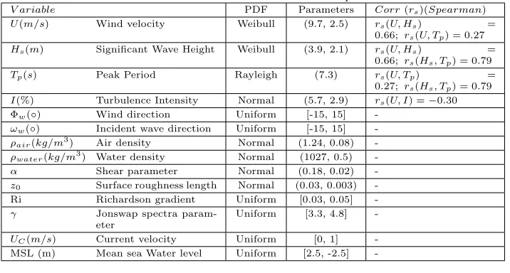
Fourteen environmental random variables were considered, n = 14, in the
representative P-GSA developed. The studied variables are presented in Table
1.
To cover the DoE, real data presented inTeixeira et al.(2018) from the M6
buoy was used to ensure a realistic approximation to the DoE environmental variables. The distributions for each input variable used in the modeling are
shown in Table1. In the cases recorded data were not available a reference study
was applied to characterize the reference intervals for the variables considered,
such as the wind profile and terrain uncertainty (Veldkamp, 2006; Jonkman,
2009;Toft et al.,2016). T¨urk and Emeis(2010) data was applied to extend the
Idataset for the height considered.
The corresponding probability papers were used to confirm the presented selection of distributions.
A Latin Hypercube Sampling (LHS) was implemented for the P-GSA proce-dure. It is important to understand that some of the variables are correlated and this influences the implementation of the LHS. Spearman correlation coefficients
between the different variables are presented in Table1. The coefficients not
presented in the table, or presented a ”very weak” correlation, or were assumed to be independent.
The correlation that exists between the θvariables considered increases the
complexity of applying the LHS. The methodology introduced in Iman and
Conover(1982) to sample correlated variables is then applied to account for the
correlation between the considered variables. Two lower triangular matricesP
andQare obtained using the Cholesky factorization of the Spearman correlation
Table 1: Random variables considered in the LHS and respective distributions V ariable PDF Parameters Corr(rs)(Spearman)
U(m/s) Wind velocity Weibull (9.7, 2.5) rs(U, Hs) = 0.66; rs(U, Tp) = 0.27
Hs(m) Significant Wave Height Weibull (3.9, 2.1) rs(U, Hs) = 0.66; rs(Hs, Tp) = 0.79
Tp(s) Peak Period Rayleigh (7.3) rs(U, Tp) =
0.27; rs(Hs, Tp) = 0.79
I(%) Turbulence Intensity Normal (5.7, 2.9) rs(U, I) =−0.30 Φw(◦) Wind direction Uniform [-15, 15]
-ωw(◦) Incident wave direction Uniform [-15, 15]
-ρair(kg/m3) Air density Normal (1.24, 0.08)
-ρwater(kg/m3) Water density Normal (1027, 0.5)
-α Shear parameter Normal (0.18, 0.02)
-z0 Surface roughness length Normal (0.03, 0.003)
-Ri Richardson gradient Uniform [0.03, 0.05]
-γ Jonswap spectra param-eter
Uniform [3.3, 4.8]
-UC(m/s) Current velocity Uniform [0, 1] -MSL (m) Mean sea Water level Uniform [2.5, -2.5]
-independently assessed LHS (T =QQ0).
R∗B=R S0 with (4)
S=P Q−1 (5)
R∗, transformed of R, has correlation matrix equal to the imposedC and
pre-serves the initial univariate distributions.
The φp(D) distance criteria introduced in Morris and Mitchell (1995) is
applied to validate the correlated and non-correlated samples and optimize dif-ferent DoEs.
Selecting an ideal sample size to perform a GSA is challenging. A minimum
sample size of n+ 1 is usually assumed for LHS, but other recommendations
are found on the adequate sample size. Iman and Helton(1985) have defined
a sample size of 4/3nas satisfactory to cover the DoE.Manache and Melching
(2008) refers that this measure was compared with the value of 3n to test its
robustness and positive results of convergence were achieved. Nevertheless many
authors do not follow strictly the rule presented inIman and Helton(1985) and
select the sample size which they believe that will produce efficient results, or for which they are investigating the adequacy. Examples can be identified in
Stein(1987) where a sample size s= 100 is used forn= 6 while Helton et al.
(2005) uses the same sample size for a n= 31.
A LHS of sizes = 30 is applied in the example presented. The criteria to
selects, additionally to requiring a minimum references within the references
presented for its selection, was to achieve adequate resolution in the variable of the space that is expected to cover a wider physical variation in absolute values,
U. Only power production (between the cut-in and cut-out wind speeds) is
3.3. Distribution ofDSH
Many natural processes are Gaussian distributed, but this is not always the case. For the case of fatigue it is commonly assumed that under constant or random loading a normal or log-normal distribution will describe accurately the
variability of the fatigue damage (Wu et al.,1997;Wirsching and Chen,1988).
To infer on the variability of DSH(Θ) the statistical output was studied
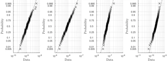
by using probability papers to compare the likelihood of different statistical distributions. The results showed that the lognormal distribution appears to
[image:7.612.164.450.257.361.2]approximate well the statistical behaviour ofDSH(Θ), Figure1. The fact that
Figure 1: Log-normal probability papers ofDSH(Θ) for 4Θcombinations.
DSH(Θ) is well represented by a lognormal distribution may be related to the
requirement forDSH to be always positive.
It is known that the logarithm of a lognormal distributed variable follows a
normal distribution. SinceDSH
DSH(Θ)∼lnN(µ, σ2).
then,
ln(DSH(Θ))∼ N(µ, σ2).
DSH(Θ) is assumed to follow a log-normal distribution∀Θ. This consideration
is important since DKL(Θ) can be represented in a closed form dependent on
continuous distributions.
100 evaluations were applied for probability characterization in order to es-timate the uncertain behavior of the tower fatigue.
4. Global Sensitivity Analysis ofDSH
4.1. Transformed sensitivity indicator.
For some physical quantities the interest is not only to characterize how far one distribution moves from one another in terms of probability, but also to characterize the physical process in regard of its practical effect. An increase in the standard deviation may contribute to a decrease in the statistical
dis-tance to a reference distribution, however in terms of practical effect (e.g. for
the reliability problem) this increase may represent a more severe operational condition and therefore should be characterized in terms of sensitivity as that.
DKL characterizes the entropy between two distributions. When using it
to characterize the distance between two distributions, it is difficult to infer on the relative location of the sensitivity point on the probabilistic map without further operations.
Consider IRµ+, IR+σ+and IRµ−, IR+σ− as separate domains of the KL function
where the change in mean and standard deviation are positive and negative respectively.
While the KL function is symmetric between its both domains,µ+ andµ−,
the same is not verified in the domainsσ+ andσ−. Similarly, the KL function
is monotonic increasing in both domains of IRµ and IR+σ−, but non-monotonic
in IR+σ+.
For engineering application purposes it may be of interest to have a com-plementary KL as a symmetric and monotonic function in all domains in order to have a more perceptive description of the P-GSA. Despite applied in previ-ous works, its original function shape has limited interest for mapping G-PSA results in practical examples, such as reliability analysis.
A transformation to the KL function is proposed in order to enable it to be an efficient indicator of G-PSA. This transformed function adds complementary
information on sensitivity toDKL that is of interest for practical applications.
To ensure a monotonic and symmetric behaviour in all the domains identified,
the KL function should be modified in IR+σ+using the following transformations
gI andgII,
gI :DKL→DIKL, ∀µf 6=µf∗ ∩ σf∗∈IR+
σ+ (6)
gI =
2DKL(σf∗=σf)
DKL(σf∗) −1 σf > σf∗≥σfmin∗
2|DKL(σf∗=σf)−DKL(σf∗=σf∗min)|
DKL(σf∗) + 1 σf
∗> σf∗
min
(7)
with σf∗
min being the value of σ
∗
f for the respective µf and µ∗f for which the
DKL is minimum. ThengII is applied accordingly to,
gII :DIKL→DKLII , ∀µf, µf∗ ∩ σf∗∈IR+
σ− (8)
gII = D
I
KL(σf+|σf−σf∗|) DKL(σf∗)
0< σf∗< σf (9)
the value of one unit as no transformation is expected,
gI = 1, ∀µf, µf∗ ∩ σf∗∈IR+
σ− ∪ σf∗=σf
, (10)
gII = 1 ∀µf, µf∗ ∩ σf∗∈IR+
σ+ ∪ σf∗ =σf, (11) This transformation could be implemented through a single transformation us-ing
[g(I−II) =gIgII] :DKL→DKLII (12)
g(I−II) is a global transformation function whilegI andgII are local
transfor-mations functions as presented in Equations (6-9). The division in a two step
function intends to facilitate the understanding of the proposed implementation.
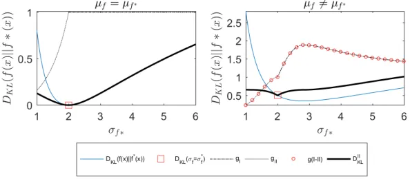
Figure 2 presents the original KL function, transformation, and the
trans-formed functions for both the cases whereµf =µf∗ andµf 6=µf∗. The second
is representative of both IRµ−and IRµ+due to the symmetry of the KL function
regarding differences inµ.
Figure 2: Example of theDKL function for the cases whenµf =µf∗ andµf 6=µf∗ for a
distribution withµf = 10 andσf = 2.
The shape of the DKL function can be identified in Figure 2. KL is not
symmetric in regard of changes in σ. When µf = µ∗f the minimum of DKL
occurs whenσf =σf∗, therefore in this caseg(I−II) =gII. Whenµf 6=µ∗f,
due to the shift caused by the difference in the means, a similar minimum for
σf =σf∗ does not occur. gI main purpose is then to guarantee that the local
minimum for∀µf 6=µf∗ occurs at σf =σf∗
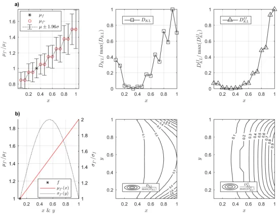
Two examples of application of DII
KL are presented in Figure 3. The first
(a) presents a univariate data set where the comparative distributionf∗ is
pro-gressively modified in relation to a reference distribution f. For the sake of
illustration, seven sets with different µand σ values are shown. For each set,
twoσvalues have been considered, i.e., the reference one and one selected
ran-domly. Even considering that the f∗ is not progressively more distant fromf
as given byDKL, its statistical moments are. The results for the discrimination
[image:9.612.152.449.328.458.2]of sensitivity to identify changes inµf∗ and inσf∗. This effect is significant as
the ratio betweenµf and µf∗ increases. When this ratio is 1.5, it can be seen
that an increase in theσf∗ results in aDKLsmaller than when this same ratio
is approximately 1.4 and the value ofσf∗closer toσf. On the other hand,DKLII
is strictly increasing as the difference between thef∗ andf moments increases.
When conducting a sensitivity analysis this is of interest in order to produce
perceptive results and should complement the analysis with DKL. When the
changes in the moments are negative,theDKLindicator increases rapidly while
DII
KL increases at the same rate of the symmetric positive changes. The second
example (b) presents a bi-variate set of data that characterizes a phenomena
where the changing behaviour ofµf∗ is mainly induced by the modification in
x, and the change in σf∗ is ruled by the y variable accordingly to the figure
presented on the left. xand y are independent and can take any value in the
field (x, y), µf∗ and σf∗ are constrained to the values taken by xandy. DKL
maxima occurs for the points where the difference inµis maxima but there is
no change inσ. DIIKLmaxima occurs for the points where the change is maxima
for both statistical moments. This example shows that, when usingDKLas an
indicator, if no further information is known about the statistical distributions it is difficult to identify accurately what are the probabilistic sensitivity results,
whileDII
KLis able to complement this analysis accurately. When the difference
in theµandσ are maxima,DKL takes the same value than when theµf∗/µf
is 1.5 with no change in σ. For some physical processes, such as loading, the
combination of two maxima is expected to be more critical. In particular, for reliability calculations, the point where both maximums occurs is the most
dan-gerous operational point because, with the same µ, more extreme values may
Figure 3: Example of implementation of KL divergence in the context of the P-GSA. a) represents a univariate set of data where both the first statistical moments are progressively increased and bothDKLandDIIKLare calculated to infer on the G-PSA. b) represents a set
of data where the sensitivities ofµand σ are mainly influence by the parametersxand y, respectively.
While the interest ofDIIKLmay not be so evident in some fields of knowledge,
such as the ones that address the need to produce probability distributions that are far from each other; in reliability engineering, it is of relevance to produce more perceptive sensitivity results. It is possible to infer that, for P-GSA in
a reliability context,DII
KL enables a more perceptive description of operational
risk, being able to complement the analysis withDKL.
In order to have a sensitivity analysis, a reference point is demanded. Appli-cation of the transformation proposed requires only the characterization of the reference distribution in order to characterize the transformed function. This
allows the characterization of theDII
KL in a single step at the beginning of the
calculations. Since the respective values for both indicators are defined, further
calculations may be performed only for DKL or DII
KL, and interpolated from
these. The numerical complexity of the sensitivity calculations may be reduced with this approach, however, its efficiency should be weighted. It may be of interest in terms of efficiency only if a very large number of points need to be
evaluated,e.g. health monitoring applications. In these cases, usage of a
required. Therefore, the approach to the P-GSA computation, its accuracy, and its numerical efficiency is expected to be case-specific.
If further information is needed aboutDKLII the local derivatives can be used
to estimate the positions in the indicator space. DIIKL may be represented in
its symmetrized form (Kullback, 1997) if a symmetric measure of sensitivity is
required. It is noted that the transformed function does not obey to the triangle
inequality in any of the cases. This same property is not respected by theDKL
orJ, and hence not by the transformed function.
4.2. G-PSA Results
The LHS generated for the set of parameters Θ is presented in Table 2.
The first two statistical moments and two results for DKL and DIIKL are also
presented in the last six columns of the table.
In the current example two reference operation points were used to compute
the G-PSA field, the hypothetical more favourable state in terms of reliability1
that could be characterized with the data generated and the real less damaging
state that was recorded (Θ= 1 in Table2). The hypothetical less damaging state
is characterized by the combination of the minimumµandσ(highlighted in bold
in Table2) possible in the data set considered. This hypothetical state is defined
with the intent of having a progressively increasing measure of sensitivity that is associated with the expected reliability for the different points of operations considered. This is an interesting reference state to use in the analysis due to its capability of producing more perceptive and practical results.
For both the DKL results, the change in the indicator is minimal. The
lower weight given to changes in the standard deviation can be identified by the
similarity between both DKL values. Examples where this indicator does not
produce perceptive results in the researched context can be found in multiple
examples, such asΘ8, 13, or 22 when comparing with the cases of 10, 14, and
24, respectively.
When consideringDII
KL,Θ18 and 22 are expected to be similar in damaging
the OWT (similar values of DSH). This is identified when considering the
minimum values of µ and σ as a reference point, however, the same does not
happen when considering Θ = 1 as a reference point. This occurs due to the
proximity ofσbetweenΘ= 1 and 22 when comparing withΘ= 18. AsDII
KL
reflects positive changes inσadditionally toµ, the difference in the divergence
between both points of operation increases while they are very likely to be similarly demanding regarding the structural fatigue of the tower component. With this example it is possible to understand that, in addition to using a perceptive measure of G-PSA, it is also of major importance when building a
DIIKL for practical problems to define a reference point that enables the most
perceptive results considering the problem analysed. In a design basis, this would help the designer to achieve more comprehensive results.
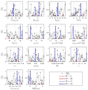
Figure 4 shows the variation of DIIKL with the univariate change of each
θi variable for the case where an hypothetical minimum state of operation is
used as reference. The four vertical lines represent, in the order shown in the
legend, the rated operation point (Θ= 11), a point with maximum indicator of
divergence (Θ= 15) and two points with small indicator of divergence (Θ= 4
& 28). These were computed for reference in order to support the comparison of results.
Figure 4: DII
KL results for each individual θivariable. Gray highlighted only purpose is to
facilitate the analysis of the results
.
The graphical analysis of the results shows one principal trend in the
uni-variate data: U as the variable in the DoE that presents a stronger indication
of being the main contributor to the definition of the probabilistic behaviour of
[image:14.612.156.448.250.548.2](11.4m/s). Operational states below the rated power have less contribution to the fatigue damage.
Iis also identified as an important variable in the DoE. There is asymmetry
in DIIKL in regard of changes in I. The gray shadow is used to facilitate the
identification of these trends. The four points with largest values ofIare located
below the ratedU, explaining the descending trend after the value of 8.7%.
I andU have a negative correlation and therefore largeU are not expected
with large I. This is one of the reasons behind the position of the most
sensitive points in the DoE, which are near the rated operation wind speed
(U = 11.4m/s). Nevertheless, if large I occurs in combination with large U,
such as inΘ= 13, the sensitivity indicator increases (in the present case
max-imum).
The transition to rated power has large influence in the results ofDSH. It
is possible to infer that there is a peak in the sensitivity measure around the rated speed that occurs independently of the values that any of the remaining
variables take. Cheng et al. (2003) showed that the largest loads in a pitch
controlled turbine occur slightly above the rated power, and these loads are expected to be related to the increase in the fatigue damage when the OWT
enters this operational region. In all the cases for similar values of U, large
values ofIresulted in larger values ofDSH. Above and below the rated power,
changes inDII
KL are mainly controlled by these two variables. By studying the
physical description of the system it is possible to understand that, whileU is
the main variable in the calculation of the average thrust moment in the OWT,
Iinfluences how the thrust fluctuates with time. LargeI is more likely to occur
with low U, where the thrust and consequently moments are lower. Despite
the increase in the Gaussian variability ofU caused by the largeI, the loading
cycles are expected to be less demanding.
The wave variables do not present any trend indicating a significant influence
in theDSH probabilistic behaviour. ForHs,Tp,ωw,ρwater,λand MSL a case
where the variable has large and small values with high and low DII
KL can be
identified, see blue and red trimmed lines. The same occurs forUC. Moreover,
for these variables, the difference in the divergence fromΘ = 18, an energetic
sea state that occurs with the maximum positive variation of MSL, andΘ =
28, a very similar sea state and variation of MSL, indicates that the response
is being dominated by the wind variables. Teixeira et al. (2017) highlighted
before the low contribution of the wave variables to the tower structural fatigue in a pre-assessment of the DoE for OWT turbines. Despite the high amount of energy that these carry, common operational waves do not directly interact and load the tower component.
In the present case it is known beforehand thatφwandωwpresent physical
symmetry with respect to the OWT. Accordingly to the results presented φw
does not seem to have major influence in the output distribution. Θ= 12 and
13, 23 and 28, are opposite symmetric where 12 and 23 represent a change in
DII
KLmore than 100% bigger than 23 and 28. The IEC standard foresees sudden
φwchange as one of the design load cases for which a OWT needs to be certified,
Accordingly to the ranges studied,z0,αandRi,ρair despite being directly
related to the wind, do not show the same influence as U and I. Both the
largest of values ρair, second largest of z0, and minimum of Ri, which would
be expected to contribute to increase DSH, result in low damage operational
states. Forαthe results are more evident in Figure5.
One of the main purposes of using a single indicator, such as DII
KL and a
minimum damaging point for reference is to map the probabilistic field using
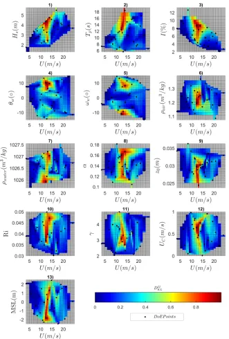
the P-GSA results in operation maps, see Figure5. This representation of the
results is interesting for dynamic systems as it allows the DoE field analysis using a sensitivity and at the same time a design basis perspective.
If with the previous figure it was challenging to be certain of the influence
of α or γ, in the map representation these seem to have limited effect in the
tower fatigue. In 8) and 11) it can be seen that the values ofDSH are mainly
occurring due to coupling with U. The map representation 3) presents the
most asymmetric behaviour inDII
KL. The largest values of DIIKLoccur near the
rated speed, and then there is a gradual increase of the indicator value with the
Figure 5: G-PSA mapping of fatigue damage operation for all the space of variables simulated (grey areas represent areas not covered by the LHS DoE).
maps. The areas of operation whereDIIKL is maximum seem to be imposed by
the values of I and U instead of the wave parameters. Furthermore, one of
the most energetic environmental wave conditions,Θ= 26, results in a smaller
change in DIIKL as the less energetic sea state, Θ = 17 (see Table 2). It is
interesting to analyse the results relating toωw for Figures4and5. According
to the symmetry, the maps indicate thatωwmay have influence on the results.
This is not supported by the other wave variable results, and therefore, may demand for more operational points to be assessed. These may be easily selected using this representation.
As U shows important influence in theDII
KL, it can be seen that in all the
maps it dominates the location of the most sensitive, thus, damaging points.
The only exception is for I, where the most damaging points are also located
at largeI values. A similar trend may appear to exist forHs. However, in the
case ofHs, considering Θ = 15, and the pairing of I and Hs in Θ = 18 and
22, there is some indication that this may be related toU andI. Furthermore,
the relative dynamics of the tower induced movement due to the coupling of the tower and foundation are small, and operation is far from the structure resonant frequencies.
In a case of highly correlated variables, such asU,Hsand Tp, the analysis
of sensitivity needs to be taken meticulous because of the coupling between variables. Due to the effect of the correlation some of the grey areas are quite
significant in the plots,e.g., plots a 1) and 3). In the context of fatigue, as a
long-term event, most of the grey areas are very unlikely to be of interest. Therefore, they should be analysed in a design basis only if relevant information about the
problem of fatigue may be held there. This may be the case of largeI andU
values.
Application of the KL to discrete datasets or using large number of eval-uation points is expected to increase the complexity of the procedure. Hence, there is consequent increase of the numerical and computational efforts required to perform it. In such cases it may be of interest to use an approximation to
continuous functions, or to interpolate from a predefinedDKLmap.
The whole probability characterization of the output is compiled in a single
variable, which characterizesDSH uncertainty. The mapping can be one of the
tools used to decide on a multi-dimensional analysis what additional points need to be addressed in order to have robust characterization results that sustain the
design decisions. The case ofωwis representative on how these maps may help
to select new points in the analysis. It is difficult by analysing Figure4or Table
2to select new points to extend the analysis since these do not allow to perceive
the DoE space.
In some particular cases, the application of the KL may be limited. In
the case of non-continuity in the compared distributions (e.g., non-overlaping distributions), the computation of KL may be challenging. Since the
proba-bilistic behaviour ofDSH was known, continuous models were used to compute
the KL. Approximation to a continuous distribution, with quantification of the error, may be a robust approach to model the KL indicator. Smoothing
alternative to deal with non-continuity in probability distributions and, hence, KL calculations. In such cases, attention should be given to the potential bias resulting from their application.
5. Conclusions
In the present work a Global Probabilistic Sensitivity Analysis was devel-oped to analyse structural fatigue sensitivity of an OWT tower. Sometimes disregarded in the field of probabilistic analysis, global sensitivity analysis are powerful methodologies to increase the comprehension about the operation of a system.
Global sensitivity analysis in a probabilistic framework allows the charac-terization of the system’s operation. In parallel, these allow the identification of important influences that the input variables may have in the probabilistic complexity of the system’s response.
When considering an engineering perspective, there are cases where the mea-sures used to compare probability distributions are of difficult interpretation, which may lead to an erroneous interpretation of the results. This fact is par-ticularly important in reliability problems where the physical meaning of the results should be considered. In this context, a transformation was proposed to the Kullback-Leibler divergence measure in order to make it more suitable for application in a probabilistic global sensitivity analysis of reliability appli-cations. The proposed transformation makes the Kullback-Leibler divergence completely symmetric and monotonic in different domains of interest in order to reflect symmetrically the sensitivity of the results. Nevertheless, only a ref-erence probability distribution is required to define the full-field transformation proposed.
The application of a measure of divergence between two statistical distribu-tions allows all the information about the probabilistic sensitivity to be compiled in a single indicator that carries information about the probability or uncertainty of the quantity studied.
Fourteen independent and dependent environmental variables that load the OWT were studied within a probabilistic reference example. A sampling tech-nique that respects the statistical interaction between variables was imple-mented to cover the space of variables.
The global sensitivity results showed that the wind speed and turbulence intensity are the most influential variables for the probabilistic short-term dam-age rates of the tower. A meticulous analysis of these variables should be always considered in the tower analysis. Both variables are correlated, and their
analy-sis cannot be disassociated. Saltelli et al.(2008) mentioned that is not unusual
that, in a high dimensional space, only few parameters show influence in the output results.
considered. Given that fatigue analysis is a cumulative event where multiple small contributions sum up to define an indicator such as the one here defined, high non-linear local effects or discontinuities are not likely to happen in the different maps. In a practical basis, the current methodology should then be implemented with a refinement strategy focusing in; global operation and then in local areas that showed relevant sensitivities or that were not adequately covered by the DoE used to characterize the full-field operation.
Acknowledgements
Notation
Di Damage indicator
DKL Kullback-Leibler divergence
DSH Short-term stress damage rate
DoE Design of Experiments
E Expected value
fY(x) Generic statistical distribution function ofY process that depends onx
fY∗(x) Generic statistical distribution function ofY∗process that depends onx g Transformation function
GSA Global Sensitivity Analysis
Hs Significant wave height (m)
I Turbulence Intensity (%)
J Symmetrized divergence KL Kullback-Leibler
LHS Latin Hypercube Sampling
NS Allowed number of stress cycles at a certain structural stress
nSti Recorded number of stress cycles at a certain structural stress in the reference timet
MSL Mean water surface level (m) OWT Offshore Wind Turbine PDF Probability Density Function
P-GSA Probabilistic Global Sensitivity Analysis
rs Spearman correlation coefficient
Ri Richardson gradient number
s Number of grid divisions
S Structural stress (Pa)
t Generic reference time
Tp Wave peak period (s)
U Mean wind speed (m/s)
UC Water current speed (m/s)
x Generic design of Experiments variablex z0 characteristic surface roughness
α Wind shear parameter
γ Wave state spectral parameter
δi moment-freemeasure of statistical divergence
∆x Imposed change in the generic variablex
θ Number of design of Experiments variables
θi Design of ExperimentsΘicomponent Θ Design of Experiments vector of variables
µ Statistical mean
µf andµ∗f mean off(x) andf
∗(x) generic statistical distributions
ρ Density (kg/m3)
σ statistical standard deviation
σf andσ∗f standard deviation off(x) andf
∗(x) generic statistical distributions
φw Wind direction angle relatively to rotor axis (◦)
ωw Incident wave direction angle relatively to rotor axis (◦)
References
Balesdent, M., Morio, J., Marzat, J., 2013. Kriging-based adaptive importance sampling al-gorithms for rare event estimation. Structural Safety 44, 1–10.
Borgonovo, E., 2007. A new uncertainty importance measure. Reliability Engineering & Sys-tem Safety 92 (6), 771–784.
Chen, S. F., Goodman, J., 1999. An empirical study of smoothing techniques for language modeling. Computer Speech & Language 13 (4), 359–394.
Cheng, P., van Bussel, G., van Kuik, G., Vugts, J., 2003. Reliability-based design methods to determine the extreme response distribution of offshore wind turbines. Wind Energy 6 (1), 1–22.
DNV, 2014. Design of offshore wind turbine structures. Offshore Standard DNV-OS-J101, DNV GL AS.
Efron, B., Stein, C., 1981. The jackknife estimate of variance. The Annals of Statistics, 586– 596.
Fatemi, A., Yang, L., 1998. Cumulative fatigue damage and life prediction theories: a survey of the state of the art for homogeneous materials. International journal of fatigue 20 (1), 9–34.
Greegar, G., Manohar, C., 2016. Global response sensitivity analysis of uncertain structures. Structural Safety 58, 94–104.
Hayman, G., 2012. Mlife theory manual for version 1.00. Tech. rep.
Helton, J. C., Davis, F., Johnson, J. D., 2005. A comparison of uncertainty and sensitivity analysis results obtained with random and latin hypercube sampling. Reliability Engineer-ing & System Safety 89 (3), 305–330.
Helton, J. C., Davis, F. J., 2003. Latin hypercube sampling and the propagation of uncertainty in analyses of complex systems. Reliability Engineering & System Safety 81 (1), 23–69.
Hoseyni, S. M., Di Maio, F., Vagnoli, M., Zio, E., Pourgol-Mohammad, M., 2015. A bayesian ensemble of sensitivity measures for severe accident modeling. Nuclear Engineering and Design 295, 182–191.
IEC, 2005. Wind turbines– part 1: Design requirements. Tech. Rep. 61400-1, International Electrotechnical Commission, Geneva, Switzerland.
Iman, R. L., Conover, W.-J., 1982. A distribution-free approach to inducing rank correlation among input variables. Communications in Statistics-Simulation and Computation 11 (3), 311–334.
Iman, R. L., Helton, J. C., 1985. Comparison of uncertainty and sensitivity analysis techniques for computer models. Tech. rep., Sandia National Labs., Albuquerque, NM (USA).
Jonkman, B. J., 2009. Turbsim user’s guide: Version 1.50.
Jonkman, J., Butterfield, S., Musial, W., Scott, G., 2009. Definition of a 5-mw reference wind turbine for offshore system development. National Renewable Energy Laboratory, Golden, CO, Technical Report No. NREL/TP-500-38060.
Kullback, S., 1997. Information theory and statistics. Courier Corporation.
Kullback, S., Leibler, R. A., 1951. On information and sufficiency. The annals of mathematical statistics 22 (1), 79–86.
Liu, H., Chen, W., Sudjianto, A., 2006. Relative entropy based method for probabilistic sensitivity analysis in engineering design. Journal of Mechanical Design 128 (2), 326–336.
Mesmacque, G., Garcia, S., Amrouche, A., Rubio-Gonzalez, C., 2005. Sequential law in mul-tiaxial fatigue, a new damage indicator. International Journal of Fatigue 27 (4), 461–467.
Morris, M. D., Mitchell, T. J., 1995. Exploratory designs for computational experiments. Journal of statistical planning and inference 43 (3), 381–402.
Olsson, A., Sandberg, G., Dahlblom, O., 2003. On latin hypercube sampling for structural reliability analysis. Structural safety 25 (1), 47–68.
Park, C. K., Ahn, K.-I., 1994. A new approach for measuring uncertainty importance and dis-tributional sensitivity in probabilistic safety assessment. Reliability Engineering & System Safety 46 (3), 253–261.
Rabitz, H., Ali¸s, ¨O. F., Shorter, J., Shim, K., 1999. Efficient input—output model represen-tations. Computer Physics Communications 117 (1-2), 11–20.
Rachev, S. T., 1991. Probability metrics and the stability of stochastic models. Vol. 269. John Wiley & Son Ltd.
Saltelli, A., Annoni, P., Azzini, I., Campolongo, F., Ratto, M., Tarantola, S., 2010. Variance based sensitivity analysis of model output. design and estimator for the total sensitivity index. Computer Physics Communications 181 (2), 259–270.
Saltelli, A., Ratto, M., Andres, T., Campolongo, F., Cariboni, J., Gatelli, D., Saisana, M., Tarantola, S., 2008. Global sensitivity analysis: the primer. John Wiley & Sons.
Saltelli, A., Tarantola, S., Campolongo, F., et al., 2000. Sensitivity anaysis as an ingredient of modeling. Statistical Science 15 (4), 377–395.
Sobol, I. M., 1993. Sensitivity estimates for nonlinear mathematical models. Mathematical Modelling and Computational Experiments 1 (4), 407–414.
Sobol, I. M., 2001. Global sensitivity indices for nonlinear mathematical models and their monte carlo estimates. Mathematics and computers in simulation 55 (1-3), 271–280.
Stein, M., 1987. Large sample properties of simulations using latin hypercube sampling. Tech-nometrics 29 (2), 143–151.
Sutherland, H. J., 1999. On the fatigue analysis of wind turbines. Tech. rep., Sandia National Labs., Albuquerque, NM (US); Sandia National Labs., Livermore, CA (US).
Teixeira, R., Nogal, M., O’Connor, A., 2018. On the suitability of the generalized pareto to model extreme waves. Journal of Hydraulic Research, 1–16.
Teixeira, R., O’Connor, A., Nogal, M., Krishnan, N., Nichols, J., 2017. Analysis of the design of experiments of offshore wind turbine fatigue reliability design with kriging surfaces. In: Procedia Structural Integrity. No. 5, 951-958.
Toft, H. S., Svenningsen, L., Sørensen, J. D., Moser, W., Thøgersen, M. L., 2016. Uncertainty in wind climate parameters and their influence on wind turbine fatigue loads. Renewable Energy 90, 352–361.
T¨urk, M., Emeis, S., 2010. The dependence of offshore turbulence intensity on wind speed. Journal of Wind Engineering and Industrial Aerodynamics 98 (8), 466–471.
Veldkamp, H. F., 2006. Chances in wind energy: a probalistic approach to wind turbine fatigue design.
Wirsching, P. H., Chen, Y.-N., 1988. Considerations of probability-based fatigue design for marine structures. Marine Structures 1 (1), 23–45.
Wu, W., Liou, H., Tse, H., 1997. Estimation of fatigue damage and fatigue life of components under random loading. International journal of pressure vessels and piping 72 (3), 243–249.
Yun, W., Lu, Z., Zhang, K., Jiang, X., 2017. An efficient sampling method for variance-based sensitivity analysis. Structural Safety 65, 74 – 83.